Division V
CASE STUDY INVESTIGATING PROBABILISTIC AND
DETERMINISTIC SAMPLING METHODS FOR DEVELOPING
IN-STRUCTURE RESPONSE SPECTRA OF A FIXED BASE IN-STRUCTURE
MODEL
Riccardo Cappa1, Frederic F. Grant2, and David K. Nakaki3
1 Staff II, Simpson Gumpertz & Heger, Inc, Newport Beach, CA, USA
2 Senior Project Manager, Simpson Gumpertz & Heger, Inc, Newport Beach, CA, USA 3 Senior Project Manager, Simpson Gumpertz & Heger, Inc, Newport Beach, CA, USA
ABSTRACT
This study compares probabilistic and deterministic seismic structural responses for a relatively simple, fixed base steel structure founded on rock. The scope of the investigation is limited to assessing the validity of the simplified deterministic sampling method that is used in practice to estimate the distribution of seismic structural responses associated with uncertainty in structure frequency.
Structural response analysis is a critical step in seismic fragility evaluation of structures, systems, and components for Seismic Probabilistic Risk Analyses (SPRAs) of nuclear power plants (NPPs). Response analyses for SPRAs typically aim to reasonably estimate median structural response quantities and associated variability. The median response quantities and variabilities are then used to develop realistic fragility curves for NPP equipment. A realistic estimate of the median seismic response and associated variability is therefore essential to realistic risk predictions in SPRAs.
Two alternative approaches are commonly considered for calculating seismic structural responses for SPRAs: a probabilistic, sampling-based approach, and a more simplified and approximate deterministic approach. Probabilistic methods consider a number of different randomized combinations of input ground motions, soil properties, and structure properties. In probabilistic analyses, a sufficient number of randomized samples are needed to achieve stable statistical results. Conversely, as a simplifying approximation, deterministic methods include fewer sample combinations of ground motions with soil and structure properties; and rather than being randomly selected, soil and structure properties are targeted at expected median and plus-and-minus one standard deviation values to estimate median and 84% non-exceedance probability (NEP) response quantities. Because deterministic results are developed from fewer statistical samples, they are less rigorous, yet they are commonly judged to reasonably approximate probabilistic results.
In this paper, probabilistic and deterministic seismic responses of a simple structure are compared in terms of median and 84% NEP in-structure response spectra (ISRS). Consistently with the scope of this paper, the two approaches are compared by including structure frequency variability as the only source of uncertainty; other sources of structure response variability (soil properties, horizontal direction peak response, structure damping, etc.) are omitted accordingly. Insights from this study are therefore limited to a narrow set of applications, but could potentially be expanded in the future to consider other sources of variability as well (e.g., soil properties). This study finds that for this simplified case where only structure frequency is varied, the deterministic approach produces very good estimates of probabilistic median and 84% NEP ISRS.
response quantities and associated variability. Variability in structure response is often quantified by developing responses at approximately 84% NEP. Both probabilistic and deterministic approaches are generally considered adequate to estimate realistic response quantities. However, deterministic results are developed from a very simplified sampling approach and thus considered less rigorous than probabilistic results.
Several studies have compared deterministic and probabilistic seismic response quantities to examine the two approaches (Elkhoraibi et al. (2011), Zinn et al. (2015), Ghiocel (2015), and Ghiocel and Stoyanov (2013)). These studies evaluated structures with various configurations and parameter distributions, and included soil-structure-interaction (SSI) effects. These studies showed that median deterministic response quantities generally compare well to probabilistic results, notwithstanding a number of exceptions. The 84% NEP demands, however, exhibited more frequent and critical discrepancies. For example, Ghiocel (2015) compared probabilistic and deterministic results for a surface founded reactor building on rock and observed that, at higher elevations, the deterministic approximations to 84% NEP horizontal ISRS were actually closer to 95% NEP. The same structure was also evaluated for soft soil conditions, and the deterministic approximations to 84% NEP horizontal ISRS at the basemat were found to be closer to 50% NEP near the peak.
Because the aforementioned studies investigated structures with various configurations, SSI features, and a number of randomized parameters, it is difficult to determine the root cause of the discrepancies between deterministic and probabilistic results. Additional studies are therefore needed to assess the adequacy of deterministic methods to develop realistic estimates.
Scope
Seismic fragility analyses implement variabilities differently depending on whether the response analysis is probabilistic or deterministic. For probabilistic response, fragility analysts generally include soil and structure variabilities (damping and frequency) and ground motion variabilities in the randomized combinations of the response analyses. Conversely, deterministic response analyses typically only vary the soil properties and structure frequency, while structure damping and ground motion variabilities are estimated independent of the response analysis. For these reasons, deterministic and probabilistic responses are not directly comparable unless the same variabilities have been incorporated. Moreover, since the deterministic uses two different techniques to implement variabilities (some “inside” and some “outside” the response analysis), it is difficult to identify which elements of the deterministic method are to blame when the results diverge from the probabilistic results.
CASE STUDY
Model
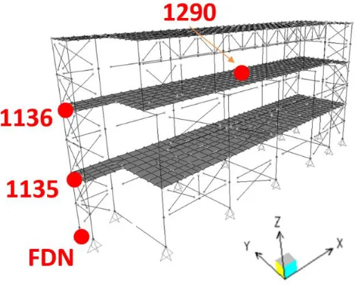
The steel structure model considered in this investigation (Figure 1) is a three-story, 53 ft tall control building (CB). The structure is relatively lightweight, has a 30 ft x 120 ft footprint, and is modelled as fixed base. The CB fundamental frequencies are 1.21 Hz and 1.55 Hz in the longitudinal (X) and transversal (Y) directions, respectively.
Figure 1 – Fixed Base, Steel Structure Model
Probabilistic Analysis
The CB probabilistic response analysis is performed using the Latin Hypercube Sampling (LHS) approach documented in NUREG/CR-2015 (Johnson et al., 1981). The only random variable included in the LHS is structure frequency, which is assumed lognormally distributed with a coefficient of variation of COVstruct,prob = 0.15. Thirty models are generated and evaluated using computer program CLASSI (Luco
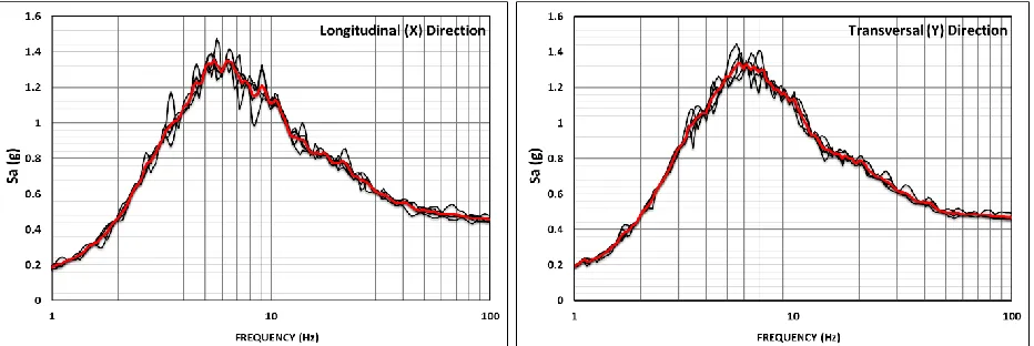
Figure 2 – 5%-damped Horizontal Response Spectra for Thirty Input THs
Figure 3 – Node 1135 5%-damped ISRS for Thirty Probabilistic Models
Deterministic Analysis
A deterministic analysis is performed to assess whether it serves as a good approximation to the probabilistic analysis. Three models are developed instead of thirty, and their structure frequency properties are targeted at median and plus-and-minus one standard deviation (COVstruct,det = 0.15) rather than being
randomly sampled. The three structure frequency case (SF) models are named best-estimate (BE), upper-bound (UB), and lower-upper-bound (LB).
Five time TH sets1 are randomly sampled from the thirty probabilistic sets (Figure 4), and ISRS are
developed for each of the five TH sets and three SFs (total of fifteen analyses). For each SF, the results of the five TH sets are then averaged to obtain the average response across multiple THs (“SFs THs averages”). For example, Figure 5(a) shows the BE THs average ISRS for Node 1135 in the X-direction. The three SFs THs averages (BE, UB, and LB) for this node and direction are shown in Figure 5(b).
The deterministic approximation to the 50% NEP ISRS is calculated as the average of the three SFs THs averages. The deterministic approximation to the 84% NEP ISRS are computed by taking the envelope of the three SFs THs averages and filling the valleys between similar modal peaks. The deterministic approximation of the 50% and 84% NEP ISRS are herein called “deterministic average” and “deterministic envelope,” respectively. These quantities are shown in Figure 5(b) for Node 1135 in the X-direction.
Figure 4 – 5%-damped Horizontal Response Spectra for Five Input THs. Red line is the average of the five THs.
Figure 5 - Node 1135 X-Direction 5%-damped ISRS for (a) Five BE THs, and (b) Three Structure Frequency Cases
Comparison of Probabilistic and Deterministic Results
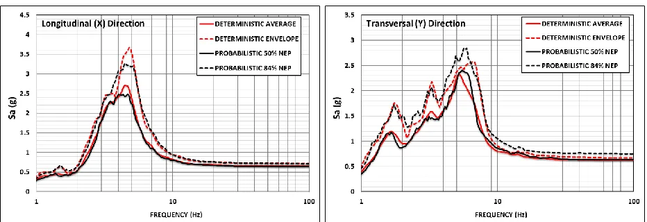
Figure 6 – Node 1135 Deterministic and Probabilistic ISRS for a) Longitudinal and b) Transversal Directions
The deterministic structural responses underestimate the probabilistic 84% NEP demands for two reasons:
A sampling bias (SB) introduced by picking five TH sets from a population of thirty. That is, some structure response uncertainty results from picking five THs because the sample statistic may not be consistent with the population. This source of variability is herein denoted as “TH SB uncertainty”.
The deterministic envelope is developed from the SFs THs averages, which do not include the randomness associated with the five different THs sets. That is, the mean response of each SF is used instead of considering the structure response variability due to TH randomness. This source of variability is herein denoted as “TH randomness”.
These two sources of variability are inherent to deterministic methodologies, and are treated in a considerably different manner in probabilistic approaches. Therefore, deterministic envelopes plotted in Figure 6 are not truly comparable to the probabilistic quantities presented in the same figure. A more appropriate comparison can be made by correcting the deterministic envelopes for both TH SB uncertainty and TH randomness. A correction methodology is developed in the following sections. The corrected deterministic envelopes are shown to be a better match to probabilistic 84% NEP demands. Deterministic averages need not be corrected since they are not considerably affected by these two sources of variability.
Correction Methodology
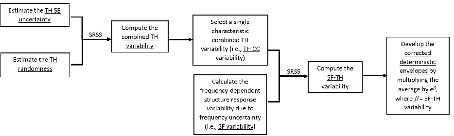
In this study, the deterministic envelopes are corrected according to the following steps (Figure 7):
A TH SB uncertainty and TH randomness are first estimated for each node and direction, and then combined as the square root of the sum of their squares (SRSS). As a simplifying approximation, the variabilities are treated as being constant across all frequencies. The combined quantity is herein called “combined TH variability”.
A single combined TH variability representative of all nodes and directions is selected based on the range of combined TH variabilities. This variability is considered characteristic of the case study investigated. This characteristic combined TH variability is herein called “TH CC variability”.
A frequency-dependent response variability (lognormal standard deviation) due to structure frequency uncertainty (herein called “SF variability”) is calculated as the natural log of the ratio of deterministic envelope to average spectral accelerations. This variability is computed for each node and direction, and combined through SRSS with the TH CC variability. The resulting joint quantity is called “SF-TH variability”.
The corrected deterministic envelopes are developed by multiplying the deterministic average by e, where β is the SF-TH variability.
Figure 7 – Correction Methodology Steps
CALCULATION OF VARIABILITIES
Time History Sampling Bias Uncertainty
For each node and direction, the TH SB uncertainty is quantified according to the following steps:
Six deterministic bins of five TH sets are randomly generated from the thirty probabilistic TH sets.
Deterministic envelopes are developed for each of the six bins, and a frequency dependent lognormal standard deviation is calculated to represent the dispersion among the six bins. This lognormal standard deviation is calculated according to Eqn. 1:
) , , , , , ( ) , , , , , ( 1 6 5 4 3 2 1 6 5 4 3 2 1 6 , Bin Bin Bin Bin Bin Bin Average Bin Bin Bin Bin Bin Bin Max LN Z SB TH
(1)where Z6 = 1.383 is the standard normal variate corresponding to the centroid of the outermost of six
equal probability bins, and Bini is the spectral acceleration of the deterministic envelope computed
using the five time history sets in the ith bin.
A constant lognormal standard deviation is estimated based on inspection of the frequency dependent lognormal standard deviation results. It is selected based on judgment to be representative of the variability at prominent peaks.
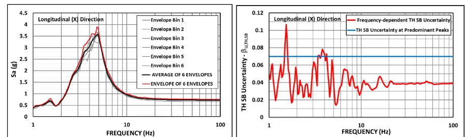
Figures 8 and 9 show sample plots used to calculate the TH SB uncertainty for Node 1135 in the X- and Y-directions, respectively. For example, the single prominent peak in the longitudinal (X) direction (Figure 8) is around 4.8 Hz, and the corresponding lognormal standard deviation capturing the variability among the six bins is estimated as TH,SB,1135-X = 0.07. The highest variability for the three peaks in the transversal
(Y) direction is around 1.8 Hz (Figure 9). For this node and direction, a TH SB uncertainty of TH,SB,1135-Y
= 0.07 is judged a reasonable estimation (Figure 9).
Figure 8 – Node 1135 Longitudinal ISRS Envelopes for Six Deterministic Bins, and Calculated TH SB Uncertainty
Figure 9 – Node 1135 Transversal ISRS Envelopes for Six Deterministic Bins, and Calculated TH SB Uncertainty
Time History Randomness
For each deterministic bin, node, and direction, the TH randomness is quantified according to the following steps:
ISRS are developed for the five THs of the BE model2.
A frequency-dependent lognormal standard deviation on the five BE THs samples is calculated according to Eqn. 2:
) , , , , ( ) , , , , ( 1 5 4 3 2 1 5 4 3 2 1 5 , TH TH TH TH TH Average TH TH TH TH TH Max LN Z Rand TH
(2)where Z5 = 1.282 is the standard normal variate corresponding to the centroid of the outermost of
five equal probability bins, and THi is the spectral acceleration of the ISRS computed from the ith
time history set.
A constant lognormal standard deviation is estimated based on inspection of the frequency dependent lognormal standard deviation results. It is selected based on judgment to be representative of the variability at prominent peaks.
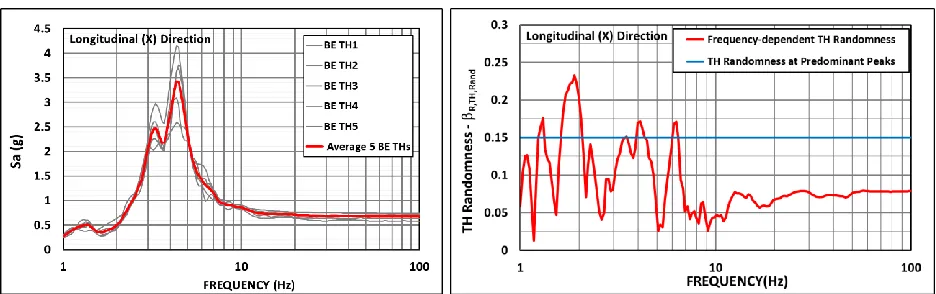
Figures 10 and 11 show sample plots used to calculate the TH randomness for Node 1135 for Bin No. 1 in the X- and Y-directions, respectively. A TH randomness of TH,Rand,1135-X = 0.15 is selected for the prominent
peaks in the 3-5 Hz range in the X-direction (Figure 10). Similarly, a variability of TH,Rand,1135-Y = 0.15 is
judged to reasonably capture the randomness for the three modal peaks in the Y-direction (Figure 11).
Figure 10 – Node 1135 Longitudinal BE ISRS for Five THs of Bin No. 1, and Calculated TH Randomness
Figure 11 – Node 1135 Transversal BE ISRS for Five THs of Bin No. 1, and Calculated TH Randomness
Combined Time History Variability
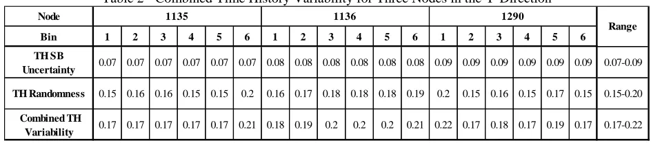
The combined TH variability is calculated as the SRSS of TH SB uncertainty and TH randomness. Tables 1 and 2 show these variabilities for three nodes (Figure 1) in the X- and Y-direction, respectively. The TH SB uncertainty is in the 0.07-0.09 range, while the TH randomness is in the 0.13-0.20 range. The combined TH variability range is 0.15-0.22 and is dominated by the TH randomness, which is consistently about twice the TH SB uncertainty. This observation suggests a strong correlation may exist between the TH SB uncertainty and TH randomness.
A sensitivity study estimated an average TH randomness of 0.05 using the ground motions of the six deterministic bins. The ISRS TH randomness presented in Tables 1 and 2 is therefore 3-4 times than that estimated at the ground. This observation confirms that TH randomness is increased as a result of structure amplification, and the increase is non-negligible. This suggests that the combined TH variability may not be accurately estimated using the ground motion TH randomness.
Table 1 – Combined Time History Variability for Three Nodes in the X-Direction Node
Bin 1 2 3 4 5 6 1 2 3 4 5 6 1 2 3 4 5 6
TH SB
Uncertainty 0.07 0.07 0.07 0.07 0.07 0.07 0.09 0.09 0.09 0.09 0.09 0.09 0.09 0.09 0.09 0.09 0.09 0.09 0.07-0.09
TH Randomness 0.15 0.15 0.13 0.15 0.15 0.14 0.18 0.19 0.18 0.17 0.19 0.15 0.17 0.2 0.15 0.15 0.18 0.16 0.13-0.20
Combined TH
Variability 0.17 0.17 0.15 0.17 0.17 0.16 0.2 0.21 0.2 0.19 0.21 0.17 0.19 0.22 0.17 0.17 0.2 0.18 0.15-0.22 Range
Characteristic Combined Time History Variability
The TH CC variability is estimated based on the values presented in Tables 1 and 2. A TH randomness of r,TH,Rand = 0.15 is first selected as a reasonable approximation for all nodes and directions.
A TH SB uncertainty of u,TH,SB = 0.08 is judged representative the 0.7-0.9 range of values calculated for
this study (Tables 1 and 2). The resulting TH CC variability is then calculated as the SRSS of these variabilities, i.e., c,TH,CC = (u,TH,SB2 + r,TH,Rand2)0.5 = 0.17. This single value is a reasonable approximation
of the 0.15-0.22 range calculated for the combined TH variabilities of all nodes and directions (Tables 1 and 2), and should be considered a characteristic of the case study investigated in this paper. The reader is cautioned that a different TH CC variability could result for different models, soil/structure properties, and ground motion inputs. In this paper, the TH CC variability of c,TH,CC = 0.17 is selected to correct the
deterministic envelopes.
Structure Response Variability due to Structure Frequency Uncertainty
The structure response variability due to structure frequency uncertainty (SF variability) corresponds to the envelope-to-average lognormal standard deviation calculated at each frequency3. This
frequency-dependent variability is calculated for each node and direction according to Eqn. 3:
Average
Envelope
LN
Z
SF 11
(3)where Z1 = 1.0 is the standard normal variate corresponding to one lognormal deviation, i.e., for three
equal probability bins, and Envelope and Average are the spectral accelerations among the three structure frequency cases.
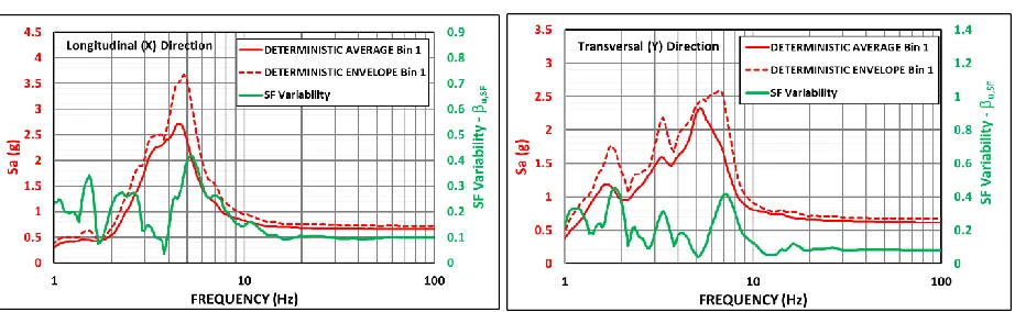
Figure 12 shows the calculation of the SF variability for Node 1135 for Bin No. 1 in both horizontal directions. The SF variability (green line) is maximum near the largest peaks, and ranges 0.08-0.10 after 11 Hz. In some frequency bands, the envelopes are close to their averages, and the SF variability drops below 0.05. For this node, the deterministic envelope tends to under-predict the 84% NEP probabilistic ISRS in those frequency regions where the SF variability is relatively low (Figure 6).
3 The reader is cautioned that drawing conclusions on response variabilities based on spectral accelerations on a
frequency basis can be misleading when differences in spectral shape are important. For example, the variability calculated according to Eqn. 3 can be very large in frequency regions where the ISRS have steep slopes (Figure 12). Lognormal standard deviations implied by peak spectral accelerations independent of the specific frequency, and at relatively high frequency bands where the ISRS flatten out are typically better estimators of the structural response variability for the purposes of seismic fragility calculations.
Figure 12 – Nodes 1135 SF Variability for Two Horizontal Directions
Structure Response-Time History Variability
Figure 13 shows the SF-TH variability computed as the SRSS of SF variability and TH CC variability for Node 1135 in both horizontal directions. The SF-TH variability (black line) is generally dominated by the SF variability (green line) near the ISRS peaks (Figure 12). The contribution of the TH CC variability (constant blue line) becomes important in those regions where the SF variability drops below 0.10, i.e., where the deterministic envelope tends to under-predict the 84% NEP probabilistic ISRS (Figure 6).
Figure 13 – Node 1135 SF and TH Variabilities for Two Horizontal Directions
COMPARISON OF PROBABILISTIC AND CORRECTED DETERMINISTIC SPECTRA
Example of Corrected Deterministic Envelope
Figure 14 illustrates the effects of the correction. The plot presents ISRS for Node 1135 in the Y-direction, and includes the probabilistic 84% NEP, the deterministic average and envelope, and the corrected deterministic envelope estimated by scaling the average by eβ, where β is the SF-TH variability.
Figure 14 – Node 1135 5%-damped 84% NEP ISRS for Probabilistic and Corrected Deterministic Estimates
Corrected Deterministic Envelope for Multiple Nodes and Directions
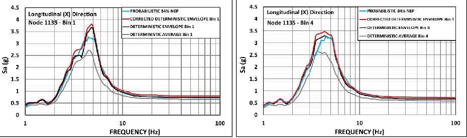
Corrected deterministic envelopes for several nodes and deterministic bins are presented in Figures 15 to 20. For a given node and direction, each figure shows the results for two of the six deterministic bins for illustration purposes. These plots suggest the corrected envelopes represent a better approximation to probabilistic 84% NEP demands compared to the original envelopes. This pattern is observed regardless of the direction, elevation, bin, or number of modes considered.
In some frequency bands, the corrected deterministic envelopes slightly overestimate the probabilistic 84% NEP demands, but the conservatism is small and should be considered commensurate with the additional uncertainty that is to be expected when using a more simplified deterministic approach rather than a rigorous probabilistic sampling method. This conservatism can be reduced, however, if a node-specific TH CC variability is used instead of a single value as in this case study.
Figure 16 – Node 1136 X-dir. 84% NEP ISRS for Probabilistic and Deterministic Bins Nos. 4 and 6
Figure 17 – Node 1290 X-dir. 84% NEP ISRS for Probabilistic and Deterministic Bins Nos. 1 and 5
Figure 18 – Node 1135 Y-dir. 84% NEP ISRS for Probabilistic and Deterministic Bins Nos. 3 and 6
Figure 20 – Node 1290 Y-dir. 84% NEP ISRS for Probabilistic and Deterministic Bins No. 1 and 6
CONCLUSIONS
This study compares probabilistic and deterministic seismic response estimates of a simple, fixed base structure founded on rock in terms of median and 84% NEP ISRS. The scope of the investigation is limited to assessing the validity of the simplified deterministic sampling method that is used in practice to estimate the distribution of seismic structural responses associated with uncertainty in structure frequency. Therefore, the deterministic and probabilistic analysis procedures investigated in this paper include structural frequency variability as the only source of parametric uncertainty. Key insights obtained from this study include the following:
Probabilistic 50% NEP demands are reasonably well estimated by deterministic averages for all nodes and directions.
Probabilistic 84% NEP demands are reasonably well estimated by deterministic envelopes, but there are a number of frequency bands where the deterministic envelopes tend to under-predict the probabilistic results.
The deterministic envelopes tend to under-predict the probabilistic 84% NEP ISRS in regions where the structure response variability due to frequency uncertainty (SF variability) is small. The under-prediction seems to be due to TH SB uncertainty and TH randomness, which are not explicitly included in the deterministic analysis methodology.
TH SB uncertainty is not currently recognized by industry practitioners as an additional source of variability in deterministic analysis. A methodology to correct deterministic estimates for TH SB uncertainty is investigated in this paper. Corrected deterministic envelopes are shown to result in a very good match of probabilistic 84% NEP ISRS.
There are frequency regions where the corrected deterministic envelopes slightly over-predict probabilistic 84% NEP ISRS. The potential conservatism introduced by accounting for additional TH variabilities is small, and is a minor penalty commensurate with the more simplified, approximate deterministic approach. This conservatism can be further reduced if a frequency-dependent combined TH variability is used instead of a constant value as in this case study.
RECOMMENDATIONS
TH SB uncertainty is an additional source of variability currently neglected in SPRA practice. For the case study investigated, the TH SB uncertainty varies between 0.07 and 0.09 and is about half of the TH randomness (Tables 1 and 2). It is therefore recommended that the TH SB variability be included in deterministic analyses. Lacking a better basis for estimating it, the TH SB variability may be estimated as roughly half of the TH randomness. Improved methods for estimating TH SB variability could potentially be developed via additional study. However, it is acknowledged that the TH SB variability is small compared to other sources considered in a fragility evaluation, and therefore the accuracy of the estimate is likely of minimal consequence to overall SPRA results.
NOTE OF CAUTION
The conclusions/recommendations of this research represent a practical application to SPRAs, but should be considered conditional to the case study investigated (relatively simple, surface founded structure with fixed base analysis, including only structure frequency uncertainty). Additional investigations are needed to assess the performance of deterministic response analysis methodologies for other building configurations, randomized parameters, and ground motion inputs.
REFERENCES
ASCE (2017), Seismic Analysis of Safety-Related Nuclear Structures, ASCE/SEI 4-16, Reston, VA. Elkhoraibi, T., Hashemi, A., and Ostadan, F. (2011), Probabilistic and Deterministic Soil Structure
Interaction Analysis Including Ground Motion Incoherency Effects, SMiRT-21, New Delhi, India. Ghiocel, D.M. and Stoyanov, G. (2013), Comparative Probabilistic-Deterministic Investigations for
Evaluation of Seismic Soil-Structure Response, SMiRT-22, San Francisco, CA.
Ghiocel, D. (2015), Probabilistic-Deterministic SSI Studies for Surface and Embedded Nuclear Structures on Soil and Rock Sites, SMiRT-23, Manchester, UK.
Johnson, J.J., et al. (1981), SMACS – Seismic Methodology Analysis Chain with Statistics, NUREG/CR-2015, Volume 9, Lawrence Livermore Laboratory, Livermore, CA.
Luco, J.E. and Wong, H.L. (1980), Soil-Structure Interaction: A Linear Continuum Mechanics Approach (CLASSI), Report No. CE79-03, University of Southern California, Los Angeles, CA.