Advanced Constitutive Model Development for Structural Integrity Analysis.

(1)

ABSTRACT

ISLAM, NAZRUL. Advanced Constitutive Model Development for Structural Integrity Analysis. (Under the direction of Dr. Tasnim Hassan).

(2)

(3)

(4)

Advanced Constitutive Model Development for Structural Integrity Analysis

by Nazrul Islam

A dissertation submitted to the Graduate Faculty of North Carolina State University

in partial fulfillment of the requirements for the degree of

Doctor of Philosophy

Civil Engineering

Raleigh, North Carolina 2018

APPROVED BY:

_______________________________ _______________________________

Dr. Tasnim Hassan Dr. Kerry Havner

Committee Chair

_______________________________ _______________________________

(5)

DEDICATION

(6)

BIOGRAPHY

(7)

ACKNOWLEDGEMENTS

I would like to thank Almighty for His blessings that allowed me to complete this thesis, and I pray that He accepts it as a work of sincerity and benefit.

I would like to express my sincere gratitude to my thesis supervisor Dr. Tasnim Hassan for his dynamic supervision, continuous guidance, invaluable suggestion and enthusiastic encouragement throughout various stages of this research. He is the best professional mentor I have ever had in my career. I am also grateful to him for the opportunities he provided me to work on the projects funded by DOE, NSF and the industries throughout the entire research.

My sincere gratitude goes to Dr. Kerry Havner for his time to meticulously reading my thesis and providing detailed corrections. I am fortunate to have such an incredible person on my thesis committee. I shall carry his invaluable suggestions in my future career and always remember him in high esteem. I would also like to thank the rest of my doctoral committee: Dr. Kumar Mahinthakumar and Dr. Gracious Ngaile for their insightful comments and the encouragement throughout this research. My sincere gratitude also goes to David J. Dewees, Advisory Engineer at Babcock and Wilcox Company, for the continuous guidance in solving recent fossil-power industry challenges.

During my studies, I have worked together with many colleagues for whom I have great regard. Among them, I wish to extend my warmest thanks to my present and previous colleagues at MANN 407, especially Dr. Shahriar Quayyum, Dr. Machel Morrison, Dr. Raasheduddin Ahmed, Dr. Paul Barrett, Graham Pritchard, Farhan Rahman, Heramb Mahajan and Urmi Devi, to name a few.

(8)

CHAPTER 5: AN IMPLICIT INTEGRATION ALGORITHM FOR FE

IMPLEMENTATION OF CONTINUUM DAMAGE COUPLED VISCOPLASTIC MODEL

Abstract ...135

2. Constitutive model ...137

3. Numerical discretization ...140

4. Numerical integration ...141

4.1. Implicit stress integration ...143

4.2. Implicit damage integration ...151

5. Numerical tests ...155

6. Conclusions ...162

7. References ...164

CHAPTER 6: DAMAGE COUPLED UNIFIED VISCOPLASTIC MODEL FOR ELEVATED TEMPERATURE APPLICATION OF GRADE 91 STEEL Abstract ...166

2. Available experimental data ...168

3.1. Kachanov damage evolution rule ...170

3.2. Isotropic damage evolution rule and its modification ...170

3.3. Creep and damage based MPC-Omega model ...172

3.4. MPC-Omega tied to Kachanov damage evolution rule ...172

4.1. Material parameters for Kachanov damage rule ...174

4.2. Material parameters for modified Isotropic damage rule ...175

4.3. Material parameters for MPC-Omega and Kachanov-Omega model ...175

5.1. Experimental and simulated responses for uniaxial fatigue (UF1) loading ...178

5.2. Experimental and simulated responses for uniaxial fatigue loading with tensile strain hold (UF2) ...182

5.3. Experimental and simulated responses for thermomechanical fatigue loading (TMF) ...182

5.4. Experimental and simulated responses for pure creep (TP2) loading ...184

5.5. Experimental and simulated responses for prior-fatigue creep (TP1) and pure creep (TP2) ...193

5.6. Experimental and simulated responses for creep (TP2) rupture life ...194

5.7. Experimental and simulated creep responses for Notch specimen ...197

(11)

CHAPTER 7: HIGH-TEMPERATURE UNIAXIAL FATIGUE, CREEP AND RATCHETING RESPONSE SIMULATION OF ALLOY 617 USING CDM COUPLED VISCOPLASTIC MODEL

Abstract ...210

2. Experiments ...212

3.1. Kachanov damage evolution rule ...218

3.2. Modified Isotropic damage evolution rule ...218

4.1. Material parameters for Kachanov damage rule ...222

4.2. Material parameters for modified Isotropic damage rule ...222

5.1. Experimental and simulated responses of Alloy 617 for uniaxial fatigue (UF1) loading ...223

5.2. Experimental and simulated responses of Alloy 617 for uniaxial fatigue loading with tensile strain hold (UF2) ...230

5.3. Fatigue-life prediction ...241

5.4. Experimental and simulated responses of Alloy 617 for uniaxial ratcheting (UR1) loading ...244

5.5. Experimental and simulated responses of Alloy 617 for uniaxial ratcheting (UR2) loading ...246

5.6. Experimental and simulated responses of Alloy 617 for pure creep (UC1) loading ...249

5.7. Creep rupture life prediction ...251

CHAPTER 8: CREEP-FATIGUE DAMAGE EVALUATION OF GRADE 91 THICK CYLINDER UNDER THERMAL TRANSIENT LOADING USING CDM COUPLED VISCOPLASTIC MODELS Abstract ...258

3. Geometry and FE model ...260

4. Heat transfer analysis ...261

5. Stress analysis ...262

5.1. FE simulations responses ...263

(12)

3. Geometry ...271

4. FE model ...272

5. Heat transfer analysis ...272

6. Stress analysis ...278

7. FE simulations responses ...279

CHAPTER 10: CONCLUSION AND FUTURE WORK 1. General ...291

2. Recommendation for future research ...294

2.1. Life-prediction method development under strain-controlled fatigue- creep interaction ...294

2.2. Life-prediction of structural components using developed constitutive model ...294

(13)

LIST OF TABLES

CHAPTER 2: EXPLICIT AND IMPLICIT INTEGRATION SCHEMES FOR FE IMPLEMENTATION OF MODIFIED-CHABOCHE BASED ELASTOPLASTIC MODEL

Table 1 : Model parameters for SS304 ... 28

Table 2 : Size and number of increments used for uniaxial strain-controlled stress- strain response simulation ... 33

Table 3 : Size and number of increments used for uniaxial stress-controlled ratcheting response simulation ... 35

Table 4 : Size and number of increments used for uniaxial strain-controlled stress- strain response simulation ... 38

CHAPTER 3: LOW CYCLE FATIGUE AND RATCHETING RESPONSE SIMULATIONS OF SS304 ELBOWS USING ADVANCED CONSTITUTIVE MODEL Table 1 : Chaboche model parameters for SS304 ... 57

Table 2 : Modified-Chaboche model parameters for SS304 ... 72

CHAPTER 4: UNIFIED AND NON-UNIFIED CONSTITUTIVE MODELS FOR PREDICTING CREEP-FATIGUE RESPONSES OF GRADE 91 STEEL Table 1 : Chaboche model parameters for modified Grade 91 steel ...109

Table 2 : Time-hardening creep coefficients for modified Grade 91 steel ...110

Table 3 : Norton’s creep coefficients for modified Grade 91 steel ...110

Table 4 : UCM power law parameters for modified Grade 91 steel ...111

Table 5 : Static recovery parameters for modified Grade 91 steel ...112

Table 6 : Modified Grade 91 LMP fitting coefficients ...113

Table 7 : API 579-1 [23] Omega (Ω) fitting coefficients [24] for modified Grade 91 steel ...116

Table 8 : Minimum strain-rate (ߝሶ_଴) fitting coefficients [24] for modified Grade 91 steel ...116

Table 9 : MPC-Omega curve-shape and primary creep coefficients for modified Grade 91 steel ...117

CHAPTER 5: AN IMPLICIT INTEGRATION ALGORITHM FOR FE IMPLEMENTATION OF CONTINUUM DAMAGE COUPLED VISCOPLASTIC MODEL Table 1 : Elastic parameters ...155

Table 2 : Kinematic hardening parameters ...155

Table 3 : Viscoplastic model parameters ...156

Table 4 : Strain-range dependent parameters ...156

Table 5 : Static recovery parameters ...157

(14)

CHAPTER 6: DAMAGE COUPLED UNIFIED VISCOPLASTIC MODEL FOR ELEVATED TEMPERATURE APPLICATION OF GRADE 91 STEEL

Table 1 : Kachanov damage evolution coefficients for the modified Grade 91

steel ...174

Table 2 : Isotropic (modified) damage evolution coefficients for the modified Grade 91 steel ...175

Table 3 : LMP fitting coefficients (WRC [14]) of modified Grade 91 steel ...176

Table 4 : Omega (Ω) fitting coefficients (API 579-1 [16]) of modified Grade 91 steel ...176

Table 5 : Minimum strain-rate (ߝሶ_଴) fitting coefficients [17] of modified Grade 91 steel ...176

Table 6 : MPC-Omega curve shape and primary creep coefficients for the modified Grade 91 steel ...177

Table 7 : MPC curve shape coefficients for Kachanov-Omega Model(proposed) for the modified Grade 91 steel ...177

Table 8 : Creep and damage parameters for the modified Grade 91 steel at T = 625°C ...199

CHAPTER 7: HIGH-TEMPERATURE UNIAXIAL FATIGUE, CREEP AND RATCHETING RESPONSE SIMULATION OF ALLOY 617 USING CDM COUPLED VISCOPLASTIC MODEL Table 1 : Chemical composition of Alloy 617 by weight (%) ...214

Table 2 : Test matrix for UF1 loading performed according to ASTM E606-04 ...215

Table 3 : Test matrix for UF2 loading performed according to ASTM E2714-09 ....215

Table 4 : Test matrix for UR1 loading performed according to ASTM E466-07 ...215

Table 5 : Test matrix for UR2 loading performed according to ASTM E466-07 ...216

Table 6 : Test matrix for UC1 loading performed according to ASTM E139-06 ...216

Table 7 : Modified Chaboche model parameters for Alloy 617 ...220

Table 8 : Shape hardening (ߛ) parameters for Alloy 617 ...221

Table 9 : Shape hardening (ܥ) parameters for Alloy 617 ...221

Table 10: Static recovery parameters for Alloy 617 at T = 900 and 1000°C ...222

Table 11: Kachanov damage evolution coefficients for Alloy 617 ...222

Table 12: Isotropic damage evolution coefficients for Alloy 617 ...223

Table 13: Primary creep parameters ...250

CHAPTER 8: CREEP-FATIGUE DAMAGE EVALUATION OF GRADE 91 THICK CYLINDER UNDER THERMAL TRANSIENT LOADING USING CDM COUPLED VISCOPLASTIC MODELS Table 1 : Analysis cases to address the effect of thick cylinder ...261

(15)

LIST OF FIGURES

CHAPTER 2: EXPLICIT AND IMPLICIT INTEGRATION SCHEMES FOR FE IMPLEMENTATION OF MODIFIED-CHABOCHE BASED ELASTOPLASTIC MODEL

Figure 1 : Schematic of kinematic hardening directions on the -plane as a function

of ′ ... 9

Figure 2 : Schematic of (a) explicit, and (b) implicit stress-return on the -plane ... 12

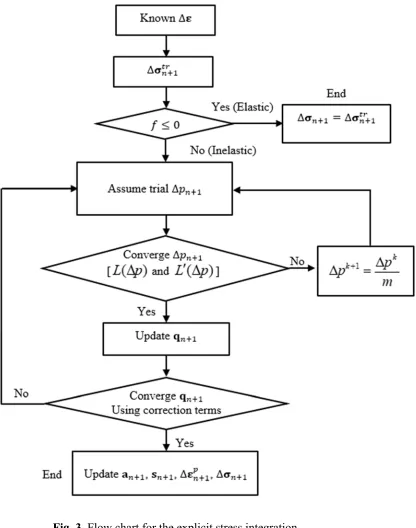
Figure 3 : Flow chart for the explicit stress integration ... 16

Figure 4 : Flow chart for the implicit stress integration ... 19

Figure 5 : Stress oscillation correction required for explicit integration method ... 27

Figure 6 : Load history for error check ... 28

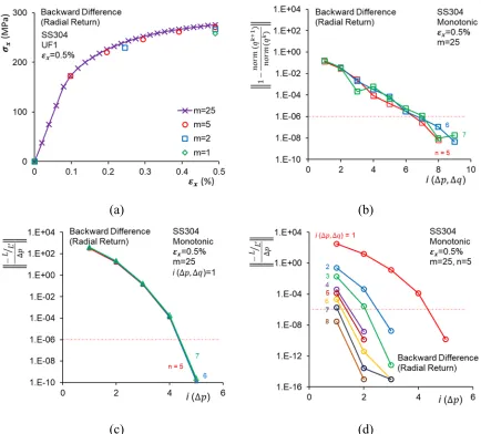
Figure 7 : Local truncation error card with 0.1%, ∆ ∆ 0.06% using forward difference method for SS304: (a) error contour; and (b) 3D error map ... 30

Figure 8 : Local truncation error card with 0.1%, ∆ ∆ 0.06% using backward difference method for SS304: (a) error contour; and (b) 3D error map ... 31

Figure 9 : Local truncation error card with 0.1%, ∆ ∆ 2% using backward difference method for SS304: (a) error contour; and (b) 3D error map ... 31

Figure 10 : Convergence of the local iteration scheme for monotonic response simulation by backward difference method: (a) effect of step-number; (b) q convergence in step 5, 6, 7; (c) ∆ convergence (local) in first iteration of step 5, 6, 7; and (d) ∆ convergence (local) in all iterations of step 5 ... 32

Figure 11 : Loading histories for (a) uniaxial fatigue, (b) uniaxial ratcheting, and (c) multiaxial ratcheting ... 33

Figure 12 : Uniaxial hysteresis loop simulation (UF1) using (a) forward difference, (b) forward difference with oscillation correction, and (c) backward difference methods ... 34

Figure 13 : Uniaxial ratcheting (UR1) stress-strain response simulation using (a) forward difference, (b) forward difference with correction, and (c) backward difference methods ... 36

Figure 14 : Uniaxial ratcheting (UR1) mean strain response simulation using (a) forward difference, (b) forward difference with correction, and (c) backward difference methods ... 37

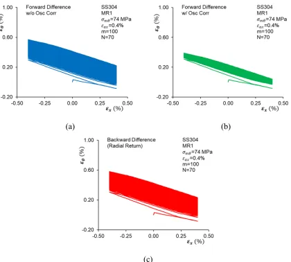
Figure 15 : Multiaxial ratcheting (MR1) circumferential-axial strain response simulation using (a) forward difference, (b) forward difference with oscillation correction, and (c) backward difference methods ... 39

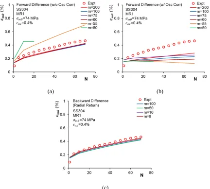
Figure 16 : Multiaxial ratcheting (MR1) mean strain response simulation using (a) forward difference, (b) forward difference with correction, and (c) backward difference methods ... 40

(16)

Figure 18 : Multiaxial strain ratcheting responses at the surface (A) of solid and shell elements: (a) hoop strain vs axial strain ; and (b) mean hoop strain vs number of cycle -N for ′ = 1 and 0.005 ... 46

CHAPTER 3: LOW CYCLE FATIGUE AND RATCHETING RESPONSE SIMULATIONS OF SS304 ELBOWS USING ADVANCED CONSTITUTIVE MODEL

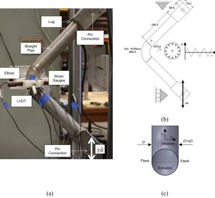
Figure 1 : Loading histories UF1, MSR, UR1, MR1 and MOP conducted by [13-16] ... 54 Figure 2 : (a) Elbow experiment set-up; (b) nominal dimensions in mm of a

long-radius elbow with boundary conditions; and (c) an elbow showing measured parameters such as diameter change (∆ ), axial ( ) and hoop ( ) strains ... 55 Figure 3 : Experimental and simulated responses of SS304 for MSR loading: (a)

stress-strain ( - ); and (b) cyclic hardening ( -N) ... 58 Figure 4 : Experimental and simulated responses of SS304 for UR1 loading: (a)

stress-strain ( - ); and (b) uniaxial ratcheting ( -N) ... 59 Figure 5 : Experimental and simulated responses of SS304 for MR1 loading: (a)

circumferential-axial strain ( - ); and (b) multiaxial ratcheting ( -N) ... 59 Figure 6 : Experimental and simulated responses of SS304 for MOP loading: (a)

torsional-axial stress (√3 ); and (b) torsional stress (√3 ) amplitude ... 60 Figure 7 : (a) FE mesh; and (b) von-Mises strain contour at the end of 120th_{cycle ... 61} Figure 8 : Experimental and simulated force-displacement (P- ) responses of long

and short-radius elbows using Chaboche stable and Chaboche with isotropic hardeing model: (a) experimental hysteresis response; (b) simulated hysteresis loop using Chaboche model with isotropic hardening; (c) mean force with cycle (Pm-N) of long-radius elbows; and (d) mean force with cycle (Pm-N) of short-radius elbows ... 64 Figure 9 : Experimental and simulated flank to flank diameter change (∆ )

responses of long and short-radius elbows using Chaboche stable and

Chaboche with isotropic hardeing model: (a) experimental diameter change (∆ - ); (b) simulated diamater change (∆ - ) using Chaboche model with isotropic hardening; (c) mean of diameter change with cycle (∆ -N) of long-radius elbows; and (d) mean of diameter change with cycle (∆ -N) of short-radius elbows ... 65

Figure 10 : Experimental and simulated circumferential strain ( ) responses at flank of long and short-radius elbows using Chaboche stable and Chaboche with isotropic hardeing model: (a) experimental circumferential strain ( - ); (b) simulated circumferential strain ( - ), using Chaboche model with isotropic hardening; (c) mean of circumferential strain with cycle ( -N) of long-radius elbows; and (d) mean of circumferential strain with cycle ( -N) of short-radius elbows ... 66 Figure 11 : Experimental and simulated circumferential strain ( ) responses at

(17)

Chaboche with isotropic hardeing model: (a) experimental circumferential strain ( - ); (b) simulated circumferential strain ( - ), using Chaboche model with isotropic hardening; (c) mean of circumferential strain with cycle ( -N) of long-radius elbows; and (d) mean of circumferential strain with cycle ( -N) of short-radius elbows ... 67 Figure 12 : Experimental and simulated axial strain ( ) responses at intrados of long

and short-radius elbows using Chaboche stable and Chaboche with isotropic hardeing model: (a) experimental axial strain ( - ); (b) simulated axial strain ( - ) using Chaboche model with isotropic

hardening; (c) mean of axial strain with cycle ( -N) of long-radius elbows; and (d) mean of axial strain with cycle ( -N) of short-radius elbows ... 68 Figure 13 : Stress-plastic strain ( - ) upgoing curve at the first cycle of each

strain-range shifted at =0.8% strain amplitude: (a) experimental; (b) prediction using isotropic hardening rule; and (c) prediction using -

hardening rule ... 71 Figure 14 : Experimental and simulated responses of SS304 for MSR loading: (a)

stress-strain ( - ); and (b) cyclic hardening ( -N) ... 73 Figure 15 : Experimental and simulated responses of SS304 for UR1 loading: (a) stress-strain ( - ); and (b) uniaxial ratcheting ( -N) ... 74 Figure 16 : Experimental and simulated responses of SS304 for MR1 loading: (a)

circumferential-axial strain ( - ); and (b) multiaxial ratcheting ( -N) ... 74 Figure 17 : Experimental and simulated responses of SS304 for MOP laoding: (a)

torsional-axial stress (√3 - ); and (b) torsional stress (√3 ) amplitude ... 75 Figure 18 : Experimental and simulated force-displacement (P- ) responses of long

and short-radius elbows using Chaboche stable and modified Chaboche models: (a) experimental hysteresis response; (b) simulated hysteresis loop; (c) mean force with cycle (Pm-N) of long-radius elbows; and (d) mean force with cycle (Pm-N) of short-radius elbows ... 77 Figure 19 : Experimental and simulated flank to flank diameter-change (∆ )

responses of long and short-radius elbows using Chaboche stable and

modified Chaboche models: (a) experimental diameter-change (∆ - ); (b) simulated diamater-change (∆ - ); (c) mean of diameter-change with cycle (∆ -N) of long-radius elbows; and (d) mean of diameter- change with cycle (∆ -N) of short-radius elbows ... 78 Figure 20 : Experimental and simulated circumferential strain ( ) responses at flank

of long and short-radius elbows using Chaboche stable and Chaboche

modified Chaboche models: (a) experimental circumferential strain ( - ); (b) simulated circumferential strain ( - ); (c) mean of circumferential strain with cycle ( -N) of long-radius elbows; and (d) mean of

circumferential strain with cycle ( -N) of short-radius elbows ... 79 Figure 21 : Experimental and simulated circumferential strain ( ) responses at

extrados of long and short-radius elbows using Chaboche stable and

(18)

); (b) simulated circumferential strain ( - ); (c) mean of circumferential strain with cycle ( -N) of long-radius elbows; and (d) mean of circumferential strain with cycle ( -N) of short-radius elbows ... 80 Figure 22 : Experimental and simulated axial strain ( ) responses at intrados of long

and short-radius elbow using Chaboche stable and modified Chaboche

models: (a) experimental axial strain ( - ); (b) simulated axial strain ( - ); (c) mean of axial strain with cycle ( -N) of long-radius elbows; and (d) mean of axial strain with cycle ( -N) of short-radius elbows ... 81 Figure 23 : Experimental and simulated responses with and without

nonproportionality: (a) mean axial strain ( -N); (b) mean

circumferential strain ( -N); and (c) circumferential vs axial stress ( - ) ... 82 Figure 24 : Schematic of strain memory surface state variables ... 83 Figure 25 : Simulated strain memory surface state variables: (a) strain memory

surface radius (q) with accumulated plastic strain (p) for UF1, UR1 and MR1 loading; (b) equivalent center location (Yeq) with accumulated plastic strain (p) for UF1, UR1 and MR1 loading; (c) q-p for MR1 loading; and (d) Yeq-p for MR1 loading ... 84 Figure 26 : Multiaxial ratcheting: (a) schematic of kinematic hardening rule; and (b)

evolution of multiaxial ratcheting parameter ... 85 Figure 27 : Experimental and simulated responses of circumferential strain for MR1

loading using modified-Chaboche model with and without evolving

multiaxial ratcheting ... 86 Figure 28 : Von-Mises strain distribution for long-radius elbow at N = 120 using (a)

stable and (b) improved models ... 86 Figure 29 : Crown section diameter-change (deformation 5X magnified) at the

closing of N = 120: (a) using stable material model; and (b) using improved model ... 87 Figure 30 : Experimental and simulated force-displacement (P- ) responses of long

and short-radius elbows using improved model: (a) experimental hysteresis response; (b) simulated hysteresis-loop; (c) force-mean with number of cycle (Pm-N) of long-radius elbows; and (d) force-mean with number of cycle (Pm-N) of short-radius elbows ... 89 Figure 31 : Experimental and simulated flank to flank diameter-change (∆ )

responses of long and short-radius elbows using improved model: (a) experimental diameter-change (∆ - ); (b) simulated diamater-change

(∆ - ); (c) mean of diameter-change with cycle (∆ -N) of long- radius elbows; and (d) mean of diameter-change with cycle (∆ -N) of short-radius elbows ... 90 Figure 32 : Experimental and simulated circumferential strain ( ) responses at flank

of long and short-radius elbows using improved model: (a) experimental

(19)

Figure 33 : Experimental and simulated circumferential strain ( ) responses at extrados of long and short-radius elbows using improved model: (a)

experimental circumferential strain ( - ); (b) simulated circumferential strain ( - ); (c) mean of circumferential strain with cycle ( -N) of long-radius elbows; and (d) mean of circumferential strain with cycle ( -N) of short-radius elbows ... 92 Figure 34 : Experimental and simulated axial strain ( ) responses at intrados of long

and short-radius elbows using improved model: (a) experimental axial strain ( - ); (b) simulated axial strain ( - ); (c) mean of axial strain with cycle ( -N) of long-radius elbows; and (d) mean of axial strain with cycle ( -N) of short-radius elbows ... 93

CHAPTER 4: UNIFIED AND NON-UNIFIED CONSTITUTIVE MODELS FOR PREDICTING CREEP-FATIGUE RESPONSES OF GRADE 91 STEEL

Figure 1 : Loading histories of experiments conducted by [13-15]: (a) uniaxial fatigue (UF1); (b) uniaxial fatigue with strain hold (UF2); (c) prior- fatigue creep (TP1); and (d) pure creep (TP2) ...102 Figure 2 : Experimental [15] and predicted responses using WRC [21] coefficients

for: (a) rupture life ; and (b) LMP ...113 Figure 3 : Experimental [15] and predicted responses using ASME coefficients for:

(a) rupture life using ASME database [22]; (b) LMP using ASME

database [22]; (c) rupture life using modified ASME coefficients; and (d) LMP using modified ASME coefficients ...114 Figure 4 : Experimental [15] and predicted responses using API 579 coefficients

for: (a) rupture life using API 579-1 database [23]; (b) LMP using API 579-1 database [23]; (c) rupture life using modified API 579-1

coefficients; and (d) LMP using modified API 579-1 coefficients ...115 Figure 5 : Experimental [15] and predicted responses for log -log using: (a) API

579-1 database [23]; (b) derived from ci’s (WRC [21]) and bi’s (API 579-1 [23]) ...116 Figure 6 : Comparison of creep models discussed in Section 3 for the responses at

T = 600°C: (a) creep (TP2) responses for = 120 MPa; and (b) rate-

dependent effect on stress-strain responses using Chab-RD model ...118 Figure 7 : Experimental and simulated responses for uniaxial fatigue loading (UF1):

(a) stress-strain hysteresis loop for 1% strain-range (N = 1, 100) at T =

600°C using Chab-RD model; (b) stress-amplitude for 0.6%, 0.8% and 1% strain-ranges at T = 600°C using Chab-RD model; (c) stress-

amplitude for 1% strain-range at T = 400, 500 and 600°C using Chab-RD model; and (d) stress-amplitude for 1% strain-range at T = 600°C using coupled and uncoupled creep-plasticity models ...119 Figure 8 : Experimental and simulated responses for uniaxial fatigue loading with

peak tensile hold (UF2) at T = 600°C: (a) stress-strain hysteresis loop (N = 1) for 1% strain-range using uncoupled models; (b) stress-strain

(20)

uncoupled and coupled creep-plasticity models ...121 Figure 9 : Experimental and simulated responses for uniaxial fatigue loading with

peak tensile hold (UF2) and pure creep (TP2) loading using uncoupled Chab-Time model at T = 600°C: (a) stress-strain hysteresis loop (N = 1) for 1% strain-range; (b) stress relaxation during hold for 1% strain-range; (c) creep responses; and (d) creep responses at an enlarged scale ...122 Figure 10 : Experimental and simulated creep responses for stress-controlled pure

creep (TP2) loading at T = 600°C using: (a) uncoupled Chab-Time model; (b) uncoupled Chab-Norton’s model; (c) uncoupled Chab-RD model; (d) uncoupled Chab-SR model ...124 Figure 11 : Experimental and simulated responses for stress-controlled pure creep

(TP2) loading at T = 450°C using uncoupled Chab-MPC model: (a) creep strain with time; and (b) creep strain-rate with creep strain ...125 Figure 12 : Experimental and simulated responses for stress-controlled pure creep

(TP2) loading at T = 500°C using uncoupled Chab-MPC model: (a) creep strain with time; and (b) creep strain-rate with creep strain ...125 Figure 13 : Experimental and simulated responses for stress-controlled pure creep

(TP2) loading at T = 550°C using uncoupled Chab-MPC model: (a) creep strain with time; and (b) creep strain-rate with creep strain ...126 Figure 14 : Experimental and simulated creep responses for stress-controlled pure

creep (TP2) loading at T = 600°C using uncoupled Chab-MPC model: (a) creep strain with time; and (b) creep strain-rate with creep strain ...126 Figure 15 : Creep rupture life and LMP prediction using Chab-MPC [21] model

plotted for: (a) log logσ; and (b) LMP logσ ...127 Figure 16 : Experimental and simulated responses for prior-fatigue creep (TP1) and

pure creep (TP2) loading: (a) creep strain using Chab-Time and Chab-

Norton’s models; (b) creep strain using Chab-RD and Chab-SR models; (c) creep strain using Chab-MPC model; and (d) stress-strain response for prior-fatigue creep using Chab-MPC model ...128

CHAPTER 5: AN IMPLICIT INTEGRATION ALGORITHM FOR FE

IMPLEMENTATION OF CONTINUUM DAMAGE COUPLED VISCOPLASTIC MODEL

Figure 1 : Radial return method on the -plane ...142 Figure 2 : Flow chart of the constitutive model ...154 Figure 3 : Load history for error check ...158 Figure 4 : Local truncation error with 0.1%, ∆ ∆ 0~2%,

10 / for Grade 91 steel at T = 600°C: (a) 3D error card; and (b) 2D error card ...159 Figure 5 : Local truncation error with 0.1%, ∆ ∆ 0~2%,

10 / for Grade 91 Steel at T = 600°C: (a) 3D error card; and (b) 2D error card ...160 Figure 6 : Load history: (a) monotonic and uniaxial fatigue; (b) uniaxial fatigue-

(21)

for UF1; (c) stress relaxation response for UF2; and (d) creep strain

responses for UC1 ...161 Figure 8 : TMF response simulations using customized UMAT in ABAQUS ...162

CHAPTER 6: DAMAGE COUPLED UNIFIED VISCOPLASTIC MODEL FOR ELEVATED TEMPERATURE APPLICATION OF GRADE 91 STEEL

Figure 1 : Loading histories of experiments conducted by [4, 8, 9] ...169 Figure 2 : Experimental and simulated stress-strain loops for UF1 loading: (a) for

∆ = 1% at T = 400°C; (b) for ∆ = 0.6%, 0.8% and 1% at T = 400°C; (c) for ∆ = 1% at T = 500°C; (d) for ∆ = 0.6%, 0.8% and 1% at T =

500°C; (e) for ∆ = 1% at T = 600°C; and (f) for ∆ = 0.6%, 0.8% and 1% at T = 600°C ...179 Figure 3 : Experimental and simulated stress amplitudes for UF1 loading at T = (a)

400°C, (b) 500°C, (c) 600°C and (d) 400, 500, 600°C ...180 Figure 4 : Experimental and simulated stress-strain hysteresis loops for UF1 loading

at T = 600°C and ∆ = 1% using UCM-CDM model with: (a) Kachanov; (b) Kachanov-Omega; (c) Isotropic [12]; and (d) modified Isotropic damage model proposed in Section 3 ...181 Figure 5 : Experiment and simulated stress-amplitude responses for UF1 loading at

T = 600°C and ∆ = 1% using UCM-CDM model with: (a) Isotropic

damage models; and (b) Kachanov, Kachanov-Omega and Isotropic damage models proposed in Section 3 ...182 Figure 6 : Experimental and simulated responses for UF2 loading: (a) - at T =

400°C; (b) - at T = 500°C; (c) - at T = 600°C; and (d) - at T = 400, 500 and 600°C ...183 Figure 7 : Experimental and simulated - (N = 1 and half cycle) for TMF

loading using UCM-CDM (Kachanov) model: (a) TMF-IP response; and (b) TMF-OP response ...183 Figure 8 : Experimental and simulated responses for TP2 loading using MPC-

Omega (including primary creep) at T = 450°C: (a) creep strain vs. time; (b) creep strain vs. time (log scale); (c) creep strain rate (log scale) vs. creep strain (log scale); and (d) creep strain rate (log scale) vs. time (log scale) ...185 Figure 9 : Experimental and simulated responses for TP2 loading using MPC-

(22)

creep strain (log scale); and (d) creep strain rate (log scale) vs. time (log scale) ...188 Figure 12 : Experimental and simulated creep strain responses for TP2 loading using

UCM-CDM (Kachanov) model at T = (a) 450°C, (b) 500°C, (c) 550°C and (d) 600°C...189 Figure 13 : Experimental and simulated creep strain responses for TP2 loading using

UCM-CDM (Kachanov-Omega) model at T = (a) 450°C, (b) 500°C, (c) 550°C and (d) 600°C ...190 Figure 14 : Experimental and simulated creep strain responses for TP2 loading using

UCM-CDM (modified Isotropic damage) model at T = (a) 450°C, (b) 500°C, (c) 550°C and (d) 600°C ...191 Figure 15 : Comparison of MPC-Omega and UCM-CDM models in predicting creep

strain at T = (a) 450°C, (b) 500°C, (c) 550°C and (d) 600°C ...192 Figure 16 : Comparison of MPC-Omega and UCM-CDM models in predicting (a)

creep strain and (b) creep damage at T = 600°C for = 110 MPa ...193 Figure 17 : Experiment and simulated responses for TP1 and TP2 using: (a) MPC-

Omega; (b) Kachanov; (c) Kachanov-Omega; and (d) Isotropic- damage models coupled with UCM ...194 Figure 18 : NIMS creep (MGC-Plate) rupture life simulation using WRC: (a)

log logσ, (b) LMP logσ ...195 Figure 19 : NIMS creep (MGC-Plate) rupture life simulation using MPC-Omega: (a)

log logσ, (b) LMP logσ ...195 Figure 20 : NIMS creep (MGC-Plate) rupture life simulation using Kachanov: (a)

log logσ, (b) LMP logσ ...196 Figure 21 : NIMS creep (MGC-Plate) rupture life simulation using Kachanov- Omega: (a) log logσ, (b) LMP logσ ...196 Figure 22 : NIMS creep (MGC-Plate) rupture life simulation using Isotropic

including triaxiality: (a) log logσ; and (b) LMP logσ ...197 Figure 23 : Geometry of the Notch by Gaffard et. al [10] ...198 Figure 24 : BC and FE mesh of a smooth specimen under creep load ...199 Figure 25 : Experimental and simulated creep strain ( ) responses of Grade 91

smooth specimen for TP2 loading at T = 625°C using UCM-CDM with: (a) Kachanov; (b) Kachanov-Omega; (c) Isotropic; and (d) modified

Isotropic damage ...200 Figure 26 : FE model, and experimental and simulation responses (at t = 150 hours,

= 218 MPa and T = 625°C) of the notch specimen: (a) BC and loading of the FE model; (b) deformation contour using UCM-CDM (Kachanov); (c) deformation contour using UCM-CDM (modified Isotropic); and (d)

using UCM-CDM (modified Isotropic) ...201 Figure 27 : Comparison of simulation responses between Kachanov and modified

Isotropic damage models: (a) creep deformation ( ) at B; (b) creep damage (D) at A; (c) von-Mises stress ( ) at A; and (d) creep strain ( ) at A ...202 Figure 28 : Experimental and simulated deformation responses of the notch specimen

(23)

and (d) modified Isotropic damage with modified triaxiality function ...203 Figure 29 : Loading histories for pure creep (CP2) and prior-fatigue creep (CP1) ...204 Figure 30 : Prior-fatigue effect on creep deformation using UCM-CDM (modified

isotropic) model: (a) for N = 0, 200 and 500, and = 150 MPa; and (b) N = 0 and 500, and = 150, 175 and 218 MPa ...205

CHAPTER 7: HIGH-TEMPERATURE UNIAXIAL FATIGUE, CREEP AND RATCHETING RESPONSE SIMULATION OF ALLOY 617 USING CDM COUPLED VISCOPLASTIC MODEL

Figure 1 : Loading histories of experiments: (a) uniaxial fatigue (UF1); (b) uniaxial fatigue with tensile strain hold (UF2); (c) uniaxial ratcheting without stress hold; (d) uniaxial ratcheting with tensile stress hold; and (e) stress- controlled pure creep (UC1) ...213 Figure 2 : Geometry of the specimen (dimensions in inch) ...214 Figure 3 : Experimental and simulated stress amplitude ( ) responses of Alloy

617 for uniaxial fatigue loading (UF1) at T = 950°C for ∆ = 0.6%, =

4x10 / and 10 / using: (a) Chaboche plasticity model; and (b)

Chaboche viscoplastic model ...224 Figure 4 : Experimental and simulated responses of Alloy 617 for uniaxial fatigue

loading (UF1) at T = 850°C: (a) - loop for ∆ = 0.6%, =

4x10 / and N = 10; (b) - loop for ∆ = 0.6%, = 4x10 / and

N = 1000; (c) for ∆ = 0.6%, = 4x10 / ; and (d) for ∆ = 0.6%, = 10 / ...225 Figure 5 : Experimental and simulated stress amplitude ( ) responses of Alloy

617 for uniaxial fatigue loading (UF1) for = 10 / at T = 850°C: (a) for ∆ = 0.3%; (b) for ∆ = 0.4%; (c) for ∆ = 0.6%; (d) for ∆ = 1%; (e) for ∆ = 2%; and (d) for ∆ = 3% ...226 Figure 6 : Coffin-Manson relationship for Alloy 617 at T = 850°C ...227 Figure 7 : Experimental and simulated responses of Alloy 617 for uniaxial fatigue

loading (UF1) at T = 950°C: (a) - loop for ∆ = 0.6%, = 10 / , and N = 10; (b) - loop for ∆ = 0.6%, = 10 / , and N = 1000; (c) - loop for ∆ = 0.4%, = 10 / , and N = 10; (d) - loop for ∆ = 0.4%, = 10 / , and N = 1000; (e) for ∆ = 0.6%, =

4x10 / and 10 / ; and (f) for ∆ = 0.6%, = 4x10 / and

10 / ...228 Figure 8 : Experimental and simulated stress amplitude ( ) responses of Alloy 617 for uniaxial fatigue loading (UF1) at T = 950°C: (a) for ∆ = 0.4%,

= 10 / ; (b) for ∆ = 0.6%; = 10 / ; (c) for ∆ = 1%, =

10 / and 10 / ; and (d) for ∆ = 2%, = 10 / and 10 / ...229 Figure 9 : Coffin-Manson relationship for Alloy 617 at T = 950°C ...230 Figure 10 : Experimental and simulated stress amplitude responses of Alloy 617 for

(24)

Figure 11 : Experimental and simulated responses of Alloy 617 for uniaxial fatigue loading with tensile strain hold (UF2) at T = 850°C for ∆ = 0.6%, =

10 / , = 60 sec: (a) stress-strain hysteresis loop for N = 10; (b) stress relaxation for N = 10; (c) stress-strain hysteresis loop for N = 500; and (d) stress relaxation for N = 500 ...232 Figure 12 : Experimental and simulated responses of Alloy 617 for uniaxial fatigue

loading with tensile strain hold (UF2) at T = 850°C for ∆ = 0.6%, =

4x10 / , = 60 sec: (a) stress-strain hysteresis loop for N = 10; (b) stress relaxation for N = 10; (c) stress-strain hysteresis loop for N = 500; (d) stress relaxation for N = 500 ...233 Figure 13 : Experimental and simulated stress amplitude of Alloy 617 for uniaxial

fatigue loading with tensile strain hold (UF2) at T = 850°C for ∆ = 0.6%, = 60 sec: (a) for = 4x10 / ; and (b) for = 10 / ...234 Figure 14 : Experimental and simulated responses of Alloy 617 for uniaxial fatigue

10 / , = 60 sec: (a) stress-strain hysteresis loop for N = 10; (b) stress relaxation for N = 10; (c) stress-strain hysteresis loop for N = 100; (d) stress relaxation for N = 100 ...235 Figure 15 : Experimental and simulated responses of Alloy 617 for uniaxial fatigue

4x10 / , = 60 sec: (a) stress-strain hysteresis loop for N = 10, (b) stress relaxation for N = 10, (c) stress-strain hysteresis loop for N = 100, (d) stress relaxation for N = 100 ...236 Figure 16 : Experimental and simulated responses of Alloy 617 for uniaxial fatigue

loading with tensile strain hold (UF2) at T = 950°C for = 60 sec: (a) stress amplitude for ∆ = 0.4%, = 4x10 / and 10 / ; and (b)

stress amplitude for ∆ = 0.6%, = 4x10 / and 10 / ...237 Figure 17 : Experimental and simulated responses of Alloy 617 for uniaxial fatigue

loading with tensile strain hold (UF2) at T = 950°C for = 10 / , = 180 sec, N = 10: (a) stress-strain hysteresis loop for ∆ = 0.6%; (b) stress relaxation for ∆ = 0.6%; (c) stress-strain hysteresis loop for ∆ = 1%; and (d) stress relaxation for ∆ = 1% ...238 Figure 18 : Experimental and simulated responses of Alloy 617 for uniaxial fatigue

loading with tensile strain hold (UF2) at T = 950°C for = 10 / , = 600 sec, N = 10: (a) stress-strain hysteresis loop for ∆ = 0.6%; (b) stress relaxation for ∆ = 0.6%; (c) stress-strain hysteresis loop for ∆ = 1%; and (d) stress relaxation for ∆ = 1% ...239 Figure 19 : Experimental and simulated responses of Alloy 617 for uniaxial fatigue

loading with tensile strain hold (UF2) at T = 950°C for = 10 / , = 1800 sec, N = 10; (a) stress-strain hysteresis loop for ∆ = 0.6%; (b) stress relaxation for ∆ = 0.6%; (c) stress-strain hysteresis loop for ∆ = 1%; (d) stress relaxation for ∆ = 1%. ...240 Figure 20 : Experimental and simulated responses of Alloy 617 for uniaxial fatigue

(25)

Figure 21 : Experimental and simulated responses of Alloy 617 for uniaxial fatigue loading with tensile strain hold (UF2) at T = 950°C for = 10 / , = 9000 sec, N = 10: (a) stress amplitude for ∆ = 0.6%; and (b) stress

amplitude for ∆ = 1% ...241 Figure 22 : Plastic strain-energy dissipation calculated from the experiment: (a) at T

= 850°C; and (b) at T = 950°C ...242 Figure 23 : Coffin-Manson relationship from the experimental and prediction: (a)

UF1 loading at T = 850°C; (b) UF1 loading at T = 950°C; and (c) UF2 loading at T = 950°C ...243 Figure 24 : Experimental responses of Alloy 617 for UF2 at T = 950°C for ∆ =

1%, = 10 / , = 180, 600, 1800 sec, N = 10: (a) hysteresis loop; and (b) stress relaxation ...244 Figure 25 : Experimental and simulated ratcheting (mean strain) responses of Alloy

617 for uniaxial ratcheting loading (UR1) at T = 850°C for = 25 MPa/s: (a) without backstress threshold model; and (b) with backstress threshold model ...245 Figure 26 : Experimental and simulated ratcheting responses of Alloy 617 for UR1

loading using the UCM-CDM (backstress threshold): (a) experimental - at T = 850°C up to N = 50; (b) simulated - at T = 850°C up to N = 50; (c) at T = 850°C; (d) at T = 950°C; (e) at T = 850°C while = 0 MPa; and (f) at T = 950°C while = 0 MPa ...247 Figure 27 : Experimental and simulated ratcheting responses of Alloy 617 for UR2

using the UCM-CDM (backstress threshold): (a) experimental - at T = 950°C up to N = 50; (b) simulated - at T = 950°C up to N = 50; (c)

at T = 850°C; (d) at T = 950°C; (e) at T = 850°C while = 0 MPa; and (f) at T = 950°C while = 0 MPa ...248 Figure 28 : Influence of static recovery on strain ratcheting: (a) experimental and

simulated strain ratcheting responses ( ) with the UCM model with and without static recovery for the first 8 cycles of an UR2 loading; and (b) experimental and simulated mean strain responses ( ) with the UCM model with and without static recovery ...249 Figure 29 : Experimental and simulated responses of Alloy 617 for stress-controlled

pure creep (UC1) at T = 900°C using UCM-CDM Model with or without primary creep ...250 Figure 30 : Experimental and simulated responses of Alloy 617 for stress-controlled

pure creep (UC1) at T = 900°C using the unified viscoplastic model: (a)

without considering static recovery and damage; (b) with static recovery but not including damage; (c) with static recovery and Kach. damage model; and (d) with static recovery and Isotropic damage ...251 Figure 31 : Experimental and simulated responses of Alloy 617 for stress-controlled

pure creep (UC1) at T = 1000°C using the unified viscoplastic model: (a) without considering static recovery and damage; (b) with static recovery but not including damage; (c) with static recovery and Kachanov damage model; and (d) with static recovery and Isotropic damage model ...252 Figure 32 : Alloy 617 creep life prediction using mod Isotropic damage coupled

(26)

stress (log logσ); and (b) developed Larson-miller parameter as a function of stress (LMP logσ) ...253

CHAPTER 8: CREEP-FATIGUE DAMAGE EVALUATION OF GRADE 91 THICK CYLINDER UNDER THERMAL TRANSIENT LOADING USING CDM COUPLED VISCOPLASTIC MODELS

Figure 1 : Thick cylinder experiment: (a) geometry; (b) FE model; (c) applied thermal loading in the experiment (Na flow) ...261 Figure 2 : Thermomechanical model parameters of the modified Grade 91 steel: (a)

thermal conductivity; (b) specific heat; and (c) thermal expansion coefficient ...262 Figure 3 : Experimental and simulated thermal responses during: (a) hot transient

loading; and (b) cold transient loading ...263 Figure 4 : FE simulation responses of the thick cylinder experiment using UCM-

CDM (modified Isotropic damage) model at N = 100 and t = 302.9 hours: (a) maximum principal strain ( ); (b) damage state variable (D); (c) von-

Mises stress ( ); and (d) simulated stress profile at inner and outer surface ...264 Figure 5 : Simulated damage at z = 0 mm ...265 Figure 6 : Comparison between simulated responses using Kachanov and modified

Isotropic damage model: (a) principal strain at N = 98~100; and (b) damage at x = 50, z = 0 mm ...265 Figure 7 : Influence of thermal cycle on: (a) strain accumulation; and (b) damage

accumulation ...266

CHAPTER 9: CREEP-FATIGUE DAMAGE EVALUATION OF GRADE 91 HEADERS UNDER FLEXIBLE OPERATION CONDITION USING CDM COUPLED VISCOPLASTIC MODELS

Figure 1 : Header geometry: (a) longitudinal section; and (b) cross-section (dimensions in mm) ...271 Figure 2 : (a) FE mesh of the quarter Header component; and (b) BC and loading

during service load ...272 Figure 3 : Measured temperature and pressure of a typical HRSG cold start-up

(Courtesy of B&W): (a) temperature; (b) internal pressure; and (c) heat transfer coefficients ...273 Figure 4 : Thermomechanical model parameters of the modified Grade 91 steel: (a)

thermal conductivity; (b) specific heat; and (c) thermal expansion coefficient ...274 Figure 5 : Typical temperature and pressure applied at the inner surface of header ..275 Figure 6 : Thermal distribution (in K) of the Header and Stub (mirror plot of the

quarter model): (a) cross section view at t = 6000 sec for type a1; (b)

isometric view at t = 6000 sec for type A1 ...276 Figure 7 : Nodal location in header and stub where a1-a6 are the nodes through the

(27)

through the thickness of header (a1-a6); (b) outer radial thermal history (b1-b5); (c) inner radial thermal history at different time interval; and (d)

comparison of outer and inner radial thermal history at t = 910 sec ...278 Figure 9 : Maximum principal strain and damage using Kachanov damage

coupled with UCM for type A1 thermal history (mirror plot) at 1st crack initiation: (a) principal strain (3D view); (b) principal strain (cross section); and (c) damage (cross section) ...280 Figure 10 : Type A1 and A2 uninterrupted service simulation results for: (a) von-

Mises stress ; (b) maximum principal strain ; (c) hoop strain ; (d) damage ; (e) ovalization ∆ ; and (f) ovalization ∆ ...283 Figure 11 : Type A2, B1 and B2 simulation results using Kachanov coupled UCM

for: (a) von-Mises stress ; (b) maximum principal strain ; (c) hoop strain ; (d) damage ; (e) ovalization ∆ ; and (f) ovalization

∆ ...284 Figure 12 : Type A2 and B1 simulation results using Kachanov-Omega coupled

UCM for: (a) von-Mises Stress ; (b) maximum principal strain ; (c) hoop strain ; (d) damage ; (e) ovalization ∆ ; and (f) ovalization

∆ ...285 Figure 13 : Type A2 and B1 simulation results using Isotropic coupled UCM for: (a)

(28)

CHAPTER 1:

INTRODUCTION

1. Background and motivation

The structural integrity of critical components (in automotive, aerospace and advanced power generation systems) subjected to extreme environmental conditions can be ensured by performing detailed component design of a system. Critical structural components such as pressure vessels, heat exchangers of the high-temperature reactors, turbine blades, components of coal-fired and nuclear power plants, etc., are subjected to adverse mechanical and thermal loading conditions over the course of their operation. The inelastic design-by-analysis of these components is often performed using the uniaxial assumption of the material model that unfortunately provides erroneous material and component response simulations. In addition, the creep-fatigue damage of such components is often analyzed using uncoupled constitutive models that can only address either fatigue or creep behavior.

(29)

2. Organization of thesis

(30)

(31)

3. References

[1] STP 1539, "Creep-Fatigue Interactions," A. Saxena and B. Dogan Eds., ASTM International, West Conshohocken, PA., (2011).

(32)

CHAPTER 2: EXPLICIT AND IMPLICIT INTEGRATION SCHEMES

FOR FE IMPLEMENTATION OF MODIFIED-CHABOCHE BASED

ELASTOPLASTIC MODEL

Abstract

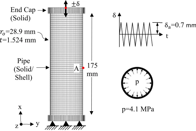
Explicit and implicit integration algorithms of a rate independent plasticity model in the modified-Chaboche kinematic hardening framework [1, 2] are developed for simulation of multiaxial fatigue-ratcheting and structural responses. Stress-return mapping and numerical solution procedures of the plasticity model are formulated based on the first order forward and backward finite difference methods, and FE implementation procedure is discussed for 3D and plane stress condition. Accuracy and stability of the model are investigated for single-step biaxial loading, uniaxial fatigue and ratcheting, and biaxial ratcheting response simulations of SS304. It has been demonstrated that the forward difference method is numerically unstable for large increment sizes, which lead to oscillations in hysteresis loop prediction. Backward difference method is found unconditionally stable in terms of uniaxial and biaxial fatigue-ratcheting responses. Formulation of the consistent tangent operator is presented for the FE implementation of the plasticity model in ANSYS USERMAT; and the FE analysis of a straight pressurized pipe under cyclic axial displacement-controlled loading is performed using the implemented constitutive model for solid and shell elements. Performance of the modified-Chaboche model is demonstrated over modified-Chaboche model [3] by comparing FE simulation responses of the straight pipe.

Keywords: Rate Independent Plasticity Model, Modified-Chaboche Model, Low Cycle Fatigue, Uniaxial Ratcheting, Multiaxial Ratcheting, Consistent Tangent Operator.

1. Introduction

(33)

of Chaboche kinematic hardening rule [7] according to Delobelle et al. [6], that incorporates Burlet-Cailletaud [2] rule, is most successful. Chaboche model [7] with four superimposed Armstrong-Frederick rules [8] improves the uniaxial ratcheting simulation; however, overprediction in biaxial ratcheting responses are observed using this model [1]. Bari and Hassan [1] implemented the Burlet-Cailletaud [2] rule in Chaboche model framework and introduced the nonlinear kinematic hardening rule, whose dynamic recovery term is the weighted scaling of regular Armstrong-Frederick’s [8] dynamic recovery along the back stress direction and radial evanescence along the plastic strain rate direction. That is, biaxial ratcheting simulation is improved by modifying the direction of dynamic recovery of the back stress. In this paper, FE implementation procedure of this modified constitutive model [1] is presented.

The FE implementation of various plasticity models has been investigated in several studies [9-13]. These studies include numerical schemes of explicit and implicit methods to solve the nonlinear incremental plasticity equations using two main approaches: 1) explicit calculation of plastic modulus satisfying the consistency condition [14], and 2) radial return scheme known as elastic predictor-plastic corrector method proposed in [15]. For both cases, Euler or higher order Runge-Kutta methods can be employed to solve the incremental equations and update the state variables.

Euler and Runge-Kutta type numerical methods are compared in [13, 16-20] to solve plasticity problems. The plasticity problems with isotropic hardening are studied by Krieg and Krieg [16] using modified Euler method, tangent-stiffness method and radial return method, and they observed that the radial return method yielded accurate predictions of monotonic loading responses. Dodds [18] also concluded that the radial return method is stable and numerically efficient compared to forward and modified Euler methods for rate-independent plasticity models (with isotropic and kinematic hardening features). Most recently, Ohno et al. [21, 22] presented implicit integration algorithms for FE implementation of Chaboche plasticity and viscoplasticity models.

(34)

hence, this study develops a robust integration algorithm for the modified-Chaboche model. The explicit and implicit integration algorithms are investigated for single-step biaxial loading, uniaxial fatigue and ratcheting, and biaxial ratcheting response simulations of SS304. The explicit integration solution scheme is found simpler but produces unstable and less accurate solutions at large increment steps due to stress oscillations. Stress scaling for this integration method is adopted following [23] to resolve stress oscillations. It has been demonstrated that the implicit integration is unconditionally stable even at large increment steps. The consistent tangent modulus for the modified-Chaboche model is derived for the implicit stress integration, which applies to both 3D and plane stress state. Finally, a numerical test is developed considering multiaxial ratcheting scenario, and simulation responses using solid and shell elements are validated for Chaboche and modified-Chaboche plasticity models.

2. Constitutive model

A rate-independent cyclic plasticity model is considered in this study for numerical implementation. The strain tensor in the framework of this plasticity model follows the additive decomposition of elastic and plastic strain. Elastic strain follows the generalized Hooke’s law and plastic strain is governed by the associative flow rule. Yield surface is represented by the von-Mises yield criterion. Kinematic hardening rule is based on modified-Chaboche model, and cyclic hardening includes hysteresis curve shape hardening.The equations of this model are shown in Eqs. (1) - (10).

Von-Mises yield criterion:





3



 

:



2

σ α s a s a _o

f      . (1)

Additive strain decomposition: e p

dεdε dε . (2)

(35)

where

1 2 2

2 1 2

2 2 1

0 0 0

0 0 0 2 0 0

0 0 0 0 2 0

0 0 0 0 0 2

k k k k k k k k k

G G G                   

Ε . (4)

Flow rule: 3 2

p

dε  dpn, (5)

where





3 2 J    s a n

σ α , and

1 2 2

: 3

p p p

dp d   d d _

 

ε ε ε .

Kinematic hardening rule: 4

1 i i





a a , (6)

where evolution of each back stress ( ) with plastic strain is given by the Modified-Chaboche model:











2 1 : 3 p

i i i i i

da  C dε  a  a n n dp. (7)

(36)

1. Note in this figure how different values of ( = 0, = 1 or 0 1) change the direction of kinematic hardening rule ( ).

Fig. 1. Schematic of kinematic hardening directions on the -plane as a function of .

In the shape hardening or -hardening modeling feature, evolves towards strain range dependent saturated value (q) with a saturation rate (Eq. 8). , and are the strain range dependent parameters for determining (q), and q and Y in Eq. (9) are the strain memory surface variables, and their evolutions are obtained by Eq. (10).

 



0



i i i i

d



D_



q 



dp, (8)

where 0

 

c qi i q ai b ei



 



_ _ 

.



 



2

: 0

3

p p

g ε Y ε Y  q . (9)

 

_: *

dq



H g n n dp, 3_{[ 1}



  

_: * *_] 2

dY   H g n n n dp, (10)

where





2 *

3

ε Y

n

ε Y

in in g

 

 .

(37)

3. Finite difference discretization

The plasticity model with the modified-Chaboche kinematic hardening rule (Eqs. 1-10) is discretized for the load increment n to n+1 as shown in Eq. (11). The discretization is made for the total stress ( ), deviatoric stress ( ), total strain ( ), plastic strain (p) and back stresses ( ).

,

1, 1,

1 1, 1 1, 1 1, 1 1,

.

a

σ

s

ε

n i

n i n i

n n n n

n n n n n n

p

n

p

n

 

       



 



 

  



 

(11)

Total stress-increment (∆ ) and deviatoric stress-increment (∆ ) at each step of strain-controlled load (∆ ) are derived from the Hooke’s law, and stress-increments are defined in Eq. (12).













1 1 1

1 1 1 1 1

: ,

: 2 .

σ E ε ε

s E e e e ε

p

n n n

D p p

n n n G n n

  

    

    

         (12)

The plastic strain-increment (∆ ) is determined from the flow rule as shown in Eq.

(13) or (14). The backstress evolution is discretized as Eq. (15) or (16).

1 1

3 2 p

n pn n

ε   n (explicit), (13)

where 3

2 ( )

n n n n n J    s a n

σ α , or

1 1 1

3 2 p

n pn n

ε   n (implicit), (14)

where 1 1

1

1 1

3

2 ( )

n n n n n J         s a n σ α .













1, 1 , , 1

2

1 :

3

a εp a a n n

n i Ci n i n i  n i n n pn

       (Forward difference), or (15)













1, 1 1, 1, 1 1 1

2

1 :

3

a εp a a n n

n i Ci n i n i  n i n n pn

(38)

The radial return mapping of the plasticity model is known as the elastic predictor-plastic corrector method. In elastic prediction, the stress is calculated elastically for a given strain increment. Then in plastic correction, the final stress increment is obtained by projecting the elastically predicted stresses on the yield surface along the direction radial to the yield surface. This return direction to the yield surface can be selected from any of the initial to updated positions of the yield surface. Based on the selected radial direction, the return mapping scheme can be an explicit (Fig. 2a) or implicit (Fig. 2b) algorithm. The explicit return mapping scheme utilizes the normal direction for the initial (nth) position of the yield surface, and back stress evolution follows forward difference discretization (Eq. 15). The implicit type return mapping scheme utilizes the normal direction from the updated yield surface and follows backward difference discretization (Eq. 16). Based on this radial direction (n+1th) and finite difference discretization of back stress evolution equation, explicit integration algorithm uses Eqs. (13) and (15), and implicit integration algorithm uses Eqs. (14) and (16). Schematic representation of the explicit and implicit algorithm is depicted in Fig. 2 showing total and back stress increment and return direction of plastic correction for stress-return mapping.

4. Stress integration

The discretization can be reduced to nonlinear scalar equations for determining the stress increment ∆ , which satisfies the discretized Eqs. (11)-(16), where all the variables are known at the beginning of the increment step. This reduction is performed in two parts, elastic prediction and plastic correction. Return mapping expressed in Eq. (17) is an elastic predictor- plastic corrector method, which is better demonstrated on the -plane shown in Fig. 2 for the explicit and implicit integration. The trial stress increment ∆ = E:∆ shown in Fig. 2 is an elastic prediction, which will satisfy the yield criterion in Eq. (18) for the plastic loading increments. To get a total stress increment ∆ , inelastic corrector term 2 ∆ is

determined based upon the yield surface . The return mapping of the inelastic corrector

2 ∆ is such that the final stress increment is calculated by projecting the elastically predicted stress point towards the radial direction of the initial (nth) or evolved (n+1th) yield surface. Now, unknown inelastic strain increment ∆ in the inelastic corrector term is a

(39)

(a) (b)

Fig. 2. Schematic of (a) explicit, and (b) implicit stress-return on the -plane.

subsequent yield surface location. Therefore, calculation of ∆ should be performed

simultaneously along with and to obtain a projection of elastic predictor on the yield surface.

1 1 1 1 1 1

σ E : ε E : ε , or σp σtr 2 ε .p

n n n n n G n

          (17)



1





1

 

1



3 _: ₀

2

tr tr tr

n n n n n n n n n o

f σ  σ _ α  s  s_ a s  s_ a   (for plastic loading). (18)

Stress-return mapping in Eq. (17) is true when all strain increments are known at the beginning of the step. But when all strain increments are not known for trial stress calculation,

a correction term ∆ is evolved, which depends on the prescription of stress or strain increments. Determination of this correction term based on stress or strain prescription is discussed in section 5. in the correction term is function of ( ), and stress-return mapping can be expressed as Eq. (19) by considering as a general term. As such, deviatoric stress in Eq. (20) can be derived from Eqs. (11), (12) and (19). Here

∆ , and is the deviatoric form of .

1

1 1 2 1 1

σ σtr εp n Q

n n n n

p G h      

      . (19)

1 2 3 ∆ ∆ +∆ ∆ ∆ ∆  ∆ 3

2∆

1 2 3 ∆ ∆ ∆ ∆ ∆ ∆ 

(40)

1

1 1 2 1 1

s str εp n QD

n n n n

p G h      

    . (20)

For the simultaneous determination of plastic strain increment (∆ ), deviatoric stress

( ), back stress ( ) and total stress increment (∆ ), nonlinear scalar equations are derived from the discretized Eqs. (11)-(16) using explicit and implicit integration methods. In the following sections, these integration algorithms and numerical solution technique of the

system of equations are demonstrated. The formulations consider correction term ∆

in a general form and depend on stress or strain prescriptions. Stress-return mapping and corrections for particular stress-strain prescriptions are demonstrated in section 5.

4.1. Explicit integration

In explicit return scheme, plastic strain increment (∆ ) can be directly obtained from

Eq. (21), where accumulated plastic strain increment (∆ ) is the root of stress-return mapping. Hence, and shown in Eqs. (22) and (23) are expanded from flow rule, stress-return, and back stress increment equations in (13), (15) and (20), and tensorial (

) is reduced to a single-valued scalar function in Eq. (25) to form a nonlinear quadratic equation (Eq. 26).

1 1 1

3 3

2 2 ( )

p n n

n n n n

n n p p J           s a ε n

σ α . (21)







