On the Decoding Failure Rate of QC-MDPC
Bit-Flipping Decoders
Nicolas Sendrier1 and Valentin Vasseur12 1
Inria, Paris, France
Universit´e Paris Descartes, Sorbonne Paris Cit´e, France.
Abstract Quasi-cyclic moderate density parity check codes [1] allow the design of McEliece-like public-key encryption schemes with compact keys and a security that provably reduces to hard decoding problems for quasi-cyclic codes.
In particular, QC-MDPC are among the most promising code-based key encapsulation mechanisms (KEM) that are proposed to the NIST call for standardization of quantum safe cryptography (two proposals, BIKE and QC-MDPC KEM).
The first generation of decoding algorithms suffers from a small, but not negligible, decoding failure rate (DFR in the order of 10−7to 10−10). This allows a key recovery attack that exploits a small correlation between the faulty message patterns and the secret key of the scheme [2], and limits the usage of the scheme to KEMs using ephemeral public keys. It does not impact the interactive establishment of secure communications (e.g.
TLS), but the use of static public keys for asynchronous applications (e.g.
email) is rendered dangerous.
Understanding and improving the decoding of QCMDPC is thus of interest for cryptographic applications. In particular, finding parameters for which the failure rate is provably negligible (typically as low as 2−64or 2−128) would allow static keys and increase the applicability of the mentioned cryptosystems.
1
Introduction
Moderate Density Parity Check (MDPC) codes were introduced for cryptography3 in [1]. They are related to Low Density Parity Check (LDPC) codes, but instead of admitting a sparse parity check matrix (with rows of small constant weight) they admit a somewhat sparse parity check matrix, typically with rows of Hamming weightO(√n) and lengthn. Together with a quasi-cyclic structure they allow the design of a McEliece-like public-key encryption scheme [4] with reasonable key size and a security that provably reduces to generic hard problems over quasi-cyclic codes, namely the hardness of decoding and the hardness of finding low weight codewords.
Because of these features, QC-MDPC have attracted a lot of interest from the cryptographic community. In particular, two key exchange mechanisms “BIKE” and “QC-MDPC KEM” were recently proposed to the NIST call for
standardization of quantum safe cryptography4.
The decoding of MDPC codes can be achieved, as for LDPC codes, with iterative decoders [5] and in particular with the (hard decision) bit flipping algorithm, which we consider here. Using soft decision decoding would improve performance [6], but would also increase the complexity and make the scheme less suitable for hardware and embedded device implementations, which is one of its interesting features [7]. There are several motivations for studying MDPC decoding. First, since QC-MDPC based cryptographic primitives may become a standard, it is worth understanding and improving their engineering and in particular the decoding algorithm, which is the bottleneck of their implementation. The other motivation is security. A correlation was established by Guo, Johansson and Stankovski in [2] between error patterns leading to a decoding failure and the secret key of the scheme: the sparse parity check matrix of a QC-MDPC code. This GJS attack allows the recovery of the secret by making millions of queries to a decryption oracle. To overcome the GJS attack, one must find instances of the scheme for which the Decoding Failure Rate (DFR) is negligible. This is certainly possible by improving the algorithm and/or increasing the code parameters, but the difficulty is not only to achieve a negligible DFR (a conservative target is a failure rate of the same order as the security requirements, that is typically 2−128) but to prove, as formally as possible, that it is negligible when the numbers we consider are out of reach by simulation.
In this work, we recall the context and the state-of-the-art in §2, mostly results of [3] as well as some new properties. In§3 we describe a new decoder, the step-by-step bit flipping algorithm, and its probabilistic model. This algorithm is less efficient than the existing techniques, but, thanks to the model, its DFR can be estimated. Finally in§4 we compare the DFR prediction of our model with the DFR obtained with simulations. We compare this with BIKE decoder
3 MDPC were previously defined, in a different context, by Ouzan and Be’ery in 2009,
http://arxiv.org/abs/0911.3262
4
simulation and try to extrapolate its behavior even when the DFR cannot be obtained by simulation.
Notation
– Throughout the paper, the matrixH∈ {0,1}r×nwill denote the sparse parity check matrix of a binary MDPC code of lengthnand dimensionk=n−r. The rows ofH, the parity check equations, have a weightw=O(√n), and are denoted eqi, 0≤i < r. The columns ofH, transposed to become row vectors, are denoted hj, 0≤j < n.
– For any binary vector v, we denoteviitsi-th coordinate and|v|its Hamming weight. Moreover, we will identify v with its support, that isi∈v if and only ifvi = 1.
– Given two binary vector u and v of same length, we will denote u∩v the set of all indices that belong to both u and v, or equivalently their component-wise product.
– The scalar product of u and v is denotedhu,vi ∈ {0,1}.
– For a random variableX we writeX ∼Bin(n, p) whenX follows a binomial distribution:
Pr[X =k] =fn,p(k) =
n
k
pk(1−p)n−k.
– In a finite state machine, the event of going from a stateS to a stateT in at mostI iterations is denoted:
S−→I T .
2
Bit Flipping Decoding
The bit flipping algorithm takes as argument a (sparse) parity check matrixH∈ {0,1}r×nand a noisy codeword y∈ {0,1}n. It flips a position if the proportion of unsatisfied equations containing that position is above some threshold. A parity check equation eqiis unsatisfied if the scalar productheqi,yi= 1. The proportion of unsatisfied equations involvingj is|s∩hj|/|hj|, where s = yHT denotes the syndrome. In practice (see [1]), the bit flipping decoder of Algorithm 1 is paralell:
Algorithm 1The Bit Flipping Algorithm Require: H∈ {0,1}(n−k)×n
, y∈ {0,1}n
whileyHT 6= 0do
s←yHT
τ←threshold(context) forj∈ {0, . . . , n−1}do
if |s∩hj| ≥τ|hj|then
yj←1−yj
the syndrome is updated after all tests and flips. The choice of a particular threshold τ depends on the context, that is H, y, and possibly anything the algorithm can observe or compute. With an appropriate choice of threshold and assuming thatHis sparse enough and y close enough to the code, the algorithm terminates with high probability.
2.1 QC-MDPC-McEliece
Bit flipping decoding applies in particular to quasi-cyclic moderate density parity check (QC-MDPC) codes which can be used in a McEliece-like encryption scheme [1]. In the cryptographic context, those codes are often of rate 1/2, length
n, dimensionk=n/2 (codimensionr=n/2). The parity matrix has row weight
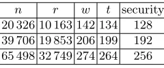
w =O(√n) and is regular (all columns have the same weightd =w/2). The bit flipping decoding correct t = O(√n) errors. Parameters n, r, w, t must be fine-tuned so that the cryptosystem is secure and the decoding failure rate (DFR) low. The implementation of Algorithm 1 for QC-MDPC was considered in several works. Different strategies have been considered so far to choose a good threshold: relying on the value of maxj(|s∩hj|/|hj|) [1], using fixed values [8] or using the syndrome weight [3, 9]. The last two strategies require, for each set of parameters, a precomputation based on simulation to extract the proper threshold selection rule. For the parameters of Table 1 those algorithms typically require less than 10 iterations for a DFR that does not exceed 10−7. Table 1 gives the sets of parameters of the BIKE proposal [10] to NIST. The bit flipping decoder of
Table 1.BIKE Parameters (security against classical adversary)
n r w t security 20 326 10 163 142 134 128 39 706 19 853 206 199 192 65 498 32 749 274 264 256
BIKE is slightly more elaborated. Its DFR appears to be below 10−10 but this is unfortunately difficult to establish from mere simulations.
2.2 A Key Recovery Attack
one needs to lower the failure rate to something negligible. Depending on the adversarial model the DFR could be a small constant, like 2−64, or even a value which decreases exponentially with the security claim (typically 2−λ forλbits of security).
2.3 Bit Flipping Identities
More details about this section can be found in [3, part III]. We assume that the MDPC code is quasi-cyclic and regular. That means that in the parity check matrixH∈ {0,1}r×n, every row has the same weightwand every column has the same weight d. Ifr=n/2, which is the most common situation in cryptographic applications, then we havew= 2d.
We consider an instance of the decoding algorithm, the noisy codeword is denoted y and is at distance t = O(√n) of the code. With probability over-whelmingly close to 1, the corresponding error e is unique. Its syndrome is s = yHT = eHT.
Definition 1. For a parity matrix H and an error vector e, the number of unsatisfied parity check equations involving the positionjisσj(e,H) =|hj∩eHT|.
We call this quantity a counter. The number of equations affected by exactly ` errors is
E`(e,H) =
n
i∈ {0, . . . , r−1}: |eqi∩e|=`
o .
The quantities e andH are usually clear form the context. We will omit them and simply writeσj andE`.
Proposition 1. The following identities are verified for all eand allH: X
` odd
E`=
eH T , X j
σj=w
eH T , X j∈e
σj=
X
`odd
`E`.
The Counter Distributions. If e is distributed uniformly among the words of weightt, we haveσj∼Bin(d, πej) with
π1=
X
`even w−1
`
n−w
t−1−`
n−1 t−1
, andπ0=
X `odd w−1 ` n−w t−` n−1 t . (1)
The above distribution is valid on average. However, the following facts are remarked in [3].
1. It does not accurately predict the counter values for an individual value of e. In fact, the counters tend to grow with the syndrome weight.
Conditioning the Counter Distributions with the Syndrome Weight. We denote
t=|e|andS=eHT
the syndrome weight. A better to model forσj is given by the distribution Bin(d, πe0
j) where (see [3])
π10 =
S+X dt , π
0 0=
(w−1)S−X
d(n−t) withX =
X
`odd
(`−1)E`. (2)
The above formulas depends on the codes parameters n, w, d, on the error weight t = |e|, on the syndrome weightS = eHT
but also on the quantity X =P
`>02`E2`+1. Here, we wish to obtain an accurate model for the counter distribution which only depends onS andt. We must somehow get rid of X. In practiceX = 2E3+ 4E5+· · · is not dominant in the above formula (for relevant QC-MDPC parameters) and we will replace it by its expected value.
Proposition 2. Wheneis chosen uniformly at random of weightt the expected value ofX =P
`>02`E2`+1 given that S=
eHT
is,
X(S, t) = S
P
`2`ρ2`+1
P
`ρ2`+1
whereρ`= w ` n−w t−` n t . Remarks.
– The counter distributions above are extremely close to the observations when the error pattern e is uniformly distributed of fixed weight.
– The model gradually degenerates as the number of iterations grows, but remains relatively accurate in the first few iterations of Algorithm 1, that is even when e is not uniformly distributed.
2.4 Adaptive Threshold
Within this model, a good threshold for Algorithm 1 isτ =T /dwhereT is the smallest integer such that (recall thatfd,πis defined in the notation)
tfd,π0
1(T)≥(n−t)fd,π00(T).
We will use this threshold selection rule in the sequel of the paper. Note that it is very consistent with the thresholds that were empirically determined in [9] to optimize Algorithm 1.
2.5 Estimating the Syndrome Weight
The probability for a parity equation eq of weightwto be unsatisfied when the error e is distributed uniformly of weightt is equal to
¯
ρ= X `odd
The syndrome weightS=eHT
is equal to the number of unsatisfied equations
and thus its expectation in ¯ρr. For a row-regular5 MDPC code the syndrome weight follows the binomial distribution Bin(r,ρ¯). However, it was remarked in [3] that for a regular MDPC code, there was a dependence between equations and the syndrome weight followed a different distribution.
In the following proposition we give the distribution of the syndrome weight when the error is uniformly distributed of weighttand the matrixH is regular.
Proposition 3. Let H be a binary r×n row-regular matrix of row weight w. When the error eis uniformly distributed of weight t, the syndrome weight S=eHT
follows the distribution
Pr[S=`] =fr,ρ(¯ `)
and if His regular of column weightd, we have
P`(t) = Pr[S=`|H is regular] = P fr,ρ(¯ `)h(`) k∈{0,...,r}fr,ρ(¯ k)h(k)
(3)
where for `∈ {0, . . . , r} (∗ is the discrete convolution operation and ∗n is the n-fold iteration of the convolution with itself )
h(`) =g∗`1 ∗g ∗(r−`) 0 (dt)
with, fork∈ {0, . . . , w},
g1(k) =
(w k)(
n−w t−k)
(n t)
1 ¯
ρ ifk is odd
0 otherwise
; g0(k) =
(w k)(
n−w t−k)
(n t)
1
1−ρ¯ if kis even
0 otherwise
.
The above distribution takes into account the regularity but not the quasi-cyclicity. Nevertheless, experimental observation shows that it is accurate for quasi-cyclic matrices, at least in the range useful for QC-MDPC codes.
3
Step-by-Step Decoding
In Algorithm 1 the positions with a counter value above the threshold are flipped all at once. In Algorithm 2 only one position is flipped at a time. The benefit, in contrast with algorithm 1, is that we can predict the evolution of the decoder. For example, when positionj with counter σj is flipped, the syndrome weight becomes|s|+|hj| −2σj. And the error weight is either increased or decreased by one.
To instanciate Algorithm 2, we will use the threshold selection rule described in§2.4 and to samplej, we uniformly pick an unverified equation then a position in this equation, that is
i← {$ i,|eqi∩y| odd};j $ ←eqi 5
Algorithm 2The Step-by-Step Bit Flipping Algorithm Require: H∈ {0,1}(n−k)×n
, y∈ {0,1}n
whileyHT 6= 0do
s←yHT
τ←threshold(context) j←sample(context) if |s∩hj| ≥τ|hj|then
yj←1−yj
returny
(wherex←$ X means we pick xuniformly at random in the setX). With this rule, and using the model for counter distributions given in§2.3, the probability to pickj∈e is
P
j0∈eσj0 P
j0σj0
=S+X
wS =
1
w
1 +X
S
,
whereS in the syndrome weight and X = 2E2+ 4E4+· · · is defined in§2.3. Note that this probability is slightly above 1/w and larger in general thant/n, the same probability whenj is chosen randomly.
3.1 Modeling the Step-by-step Decoder
We assume here thatHis the sparse parity check matrix of a regular QC-MDPC code, with row weightwand column weightd. We model the step-by-step decoder as a finite state machine (FSM) with a state (S, t) withS the syndrome weight andt the error weight.
We consider one loop of Algorithm 2. The positionj is sampled, the corres-ponding counter value is denotedσ=|s∩hj|and the threshold isT =τ|hj|=τ d. There are 3 kinds of transition,
– ifσ < T, then (S, t)→(S, t), with probability p
– ifσ≥T andj∈e, then (S, t)→(S+d−2σ, t−1), with probabilityp−σ
– ifσ≥T andj6∈e, then (S, t)→(S+d−2σ, t+ 1), with probabilityp+σ and the transition probabilities are given in the following proposition.
Proposition 4.
p−σ = tσfd,π
0 1(σ)
wS , p
+ σ =
(n−t)σfd,π0 0(σ)
wS , p= X
σ<T
(p−σ +p+σ),
wherefd,π(i) = di
πi(1−p)d−i andπ0
0, π10 are given in (2) in§2.3.
The above machine does not correctly take into account the situation where the algorithm is unable to find a suitable position to flip. We modify it as follows: one step of the new machine will iterate the loop until a flip occurs. We callj
– if no high enough counter is found, then (S, t)→L, with probabilitypL
– ifσ≥T andj∈e, then (S, t)→(S+d−2σ, t−1), with probabilityp0−σ
– ifσ≥T andj6∈e, then (S, t)→(S+d−2σ, t+ 1), with probabilityp0+ σ
where the state L corresponds to the situation where there no position exists with a suitable counter.
Proposition 5.
p0−σ =p−σ1−pL
1−p, p
0+ σ =p
+ σ
1−pL 1−p , wherep, p−σ, p+σ are given in Proposition 4, and
pL =
X
σ<T
fd,π0 1(σ)
!t
· X
σ<T
fd,π0 0(σ)
!n−t ,
wherefd,π(i) = diπi(1−p)d−i andπ00, π10 are given in (2) in§2.3.
Note. As mentionned in§2.3, we have replacedX by X (Proposition 2) inπ00, π10
in all the results of this section.
3.2 Computing the DFR
To compute the theoretical DFR in our model, we will add another state F corresponding to a decoding failure. We assume the stochastic process we have defined in the previous section is a time-homogeneous Markov chain. For any starting state (S, t) we wish to determine with which probability the FSM reaches the failure state after an infinite number of iterations:
DFR(S, t) = Pr[(S, t)−→∞ F].
Since we assumed an infinite number of iterations, we need to fix an error weight above which the decoder fails, saytfail. Similarly, to simplify the computation, we assume that whentis small enough, say belowtpass the decoder always succeeds. We have ∀t≤tpass,Pr[(S, t)
∞
−→F] = 0 and∀t > tfail,Pr[(S, t) ∞
−→F] = 1. Notice that as long asT ≥d+1
2 (which is always the case here),∀σ≥T, Sσ< S therefore these probabilities can be computed by induction with S in ascending order. Finally, the probability to successfully decode a vector y noised with a uniformly distributed error of weighttin the model is
DFR(t) =X S
PS(t) DFR(S, t)
3.3 Using t Alone for the State is not Enough
In the analysis of LDPC decoding, starting with Gallager’s work [5], it is usually assumed that the error pattern remains uniformly distributed throughout the decoding process. This assumption greatly simplifies the analysis. It is correct for LDPC codes, but unfortunately not for MDPC codes.
Assuming uniform distribution of the error during all the decoding is equivalent to adopting a stochastic model in which the decoder state is described by the error weight alone. From our analysis, we easily derive the transition probabilities as
Pr[t→(t±1)] =X S
PS(t)X S0
Pr[(S, t)→(S0, t±1)].
The corresponding Markov chain can be computed. We observe a huge discrepancy. For instance, for parameters (n, r, w, t) = (65500,32750,274,264) the observed failure rate is in the order of 10−4 for the step-by-step decoder while the model predicts less than 10−12. The difference is even higher for larger block size.
4
Simulation
We simulate here three algorithms:
Algorithm 1: as in [3], using the threshold selection rule of§2.3.
Algorithm 2: step-by-step bit flipping as in the model of§3.
BIKE decoder: adapted from [10].
The parameters are those of BIKE-1 Level 5 (d= 137,w= 274,t= 264) with rate 1/2 and a varying block sizer.
The true BIKE decoder is tuned forr= 32749. We adapt it here for variable
r. The BIKE decoder starts with one iteration of Algorithm 1 and ends with Algorithm 2 and a thresholdτ = 0.5. Between the two there a “gray zone” step described in [10].
Let us point out that the threshold selection rule of§3 (used for Algorithms 1 and 2 and the model is not honest. It assumes that the error weight is known throughout the computation while obviously a real decoder has no access to that information. However the main objective here was to compare the simulation and the model, and both of them “cheat”. Moreover, we believe that finding the “good” threshold can always be achieved for an extra computational cost without cheating. Note finally that the BIKE algorithm outperform the others without relying on the knowledge of the error weight.
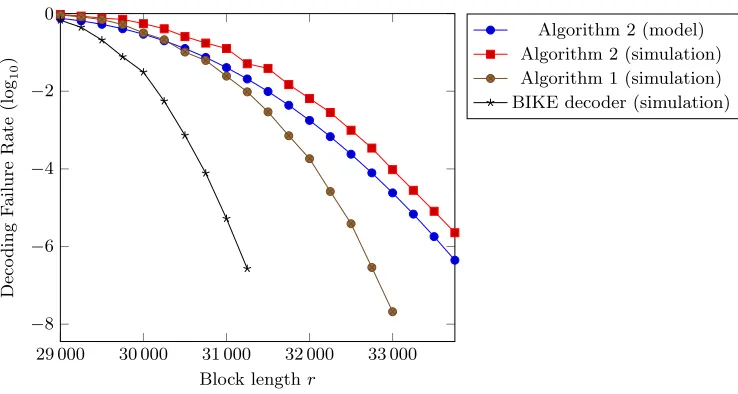
In figure 1, we compare the DFR derived from our model to the one obtained by Monte Carlo simulations of the three above decoders.
29 000 30 000 31 000 32 000 33 000 −8
−6 −4 −2 0
Block lengthr
Deco
d
ing
F
ailure
Rate
(log
10
)
Algorithm 2 (model) Algorithm 2 (simulation) Algorithm 1 (simulation) BIKE decoder (simulation)
Figure 1. DFR of the step-by-step algorithm in the models and from simulations (infinite number of iterations)
range plotted in Figure 1, we have noticed that the DFR evolves in two phases, in the first phase (r <37 500) it closely fits a quadratic curve and in the second phase it is linear, which is consistent with the asymptotic analysis in [11].
Table 2.Extrapolating QC-MDPC Parameters
(a) (b) (c) (d) (e) (f) Algorithm 1−21.6−21.6 35 498 39 652 34 889 36 950
BIKE −48.8−57.0 33 594 37 149 32 983 34 712 Algorithm 2−10.4−11.5 39 190 46 884 37 537 40 952
(a): linearly extrapolated value for log2(pfail(32 749)); (b): quadratically extrapolated value for log2(pfail(32 749));
(c): minimalrsuch thatpfail(r)<2−64 assuming a linear evolution; (d): minimalrsuch thatpfail(r)<2−128 assuming a linear evolution; (e): minimalrsuch thatpfail(r)<2−64 assuming a quadratic evolution; (f): minimalrsuch thatpfail(r)<2−128 assuming a quadratic evolution
5
Conclusion
We have presented here a variant of the bit flipping decoder of QC-MDPC codes, namely the step-by-step decoder. It is less efficient than the existing decoders, but can be accurately modeled by a Markov chain. If we assume that the evolution of the DFR of other related algorithms, and in particular BIKE, follow the same kind of evolution, we are able to give estimates for their DFR and also of the block size we would need to reach a low enough error rate. For BIKE-1 level 5, we estimate the DFR between 2−49and 2−57. As shown in Table 2, the amount by which the block size should be increased to reach a DFR of 2−64 or even 2−128seems to be relatively limited, only 1% to 15%. This suggest that with an improvement of the decoder efficiency, the original BIKE parameters might not to far to what is needed for resisting the GJS attack and allow static keys.
References
1. Misoczki, R., Tillich, J.P., Sendrier, N., Barreto, P.S.L.M.: MDPC-McEliece: New McEliece variants from moderate density parity-check codes. In: Proc. IEEE Int. Symposium Inf. Theory - ISIT. (2013) 2069–2073
2. Guo, Q., Johansson, T., Stankovski, P.: A key recovery attack on MDPC with CCA security using decoding errors. In Cheon, J.H., Takagi, T., eds.: Advances in Cryptology - ASIACRYPT 2016. Volume 10031 of LNCS. (2016) 789–815 3. Chaulet, J.: ´Etude de cryptosyst`emes `a cl´e publique bas´es sur les codes MDPC
quasi-cycliques. PhD thesis, University Pierre et Marie Curie (March 2017) 4. McEliece, R.J. In: A Public-Key System Based on Algebraic Coding Theory. Jet
Propulsion Lab (1978) 114–116 DSN Progress Report 44.
5. Gallager, R.G.: Low Density Parity Check Codes. M.I.T. Press, Cambridge, Massachusetts (1963)
6. Baldi, M., Santini, P., Chiaraluce, F.: Soft mceliece: MDPC code-based mceliece cryptosystems with very compact keys through real-valued intentional errors. In: Proc. IEEE Int. Symposium Inf. Theory - ISIT, IEEE Press (2016) 795–799 7. Heyse, S., von Maurich, I., G¨uneysu, T.: Smaller keys for code-based cryptography:
QC-MDPC McEliece implementations on embedded devices. In Bertoni, G., Coron, J., eds.: Cryptographic Hardware and Embedded Systems - CHES 2013. Volume 8086 of LNCS., Springer (2013) 273–292
8. Chou, T.: Qcbits: Constant-time small-key code-based cryptography. In Gierlichs, B., Poschmann, A.Y., eds.: CHES 2016. Volume 9813 of LNCS., Springer (2016) 280–300
9. Chaulet, J., Sendrier, N.: Worst case QC-MDPC decoder for mceliece cryptosystem. In: IEEE Conference, ISIT 2016, IEEE Press (2016) 1366–1370
10. Aguilar Melchor, C., Aragon, N., Barreto, P., Bettaieb, S., Bidoux, L., Blazy, O., Deneuville, J.C., Gaborit, P., Gueron, S., G¨uneysu, T., Misoczki, R., Persichetti, E., Sendrier, N., Tillich, J.P., Z´emor, G.: BIKE. first round submission to the NIST post-quantum cryptography call (November 2017)
A
Precisions on
§
2.5
Let us write ωi = |eqi∩e| for all row 0 ≤ i < r. Then S =
P
i(ωi mod 2). Moreover, for a regular code, theωivariables always verify the following property:
X
i∈{0,...,r−1}
ωi=d· |e|.
We wish to determine the distribution ofP
i∈{0,...,r−1}ωi knowing the syn-drome weight. We can then apply the Bayes’ theorem to obtain the result of proposition 3:
Pr[S=`|His regular] = Pr[S =`|P
i∈{0,...,r−1}ωi=d|e|] = Pr[
P
i∈{0,...,r−1}ωi=d|e| |S =`] Pr[S =`] Pr[P
i∈{0,...,r−1}ωi=d|e|]
= Pr[
P
i∈{0,...,r−1}ωi=d|e| |S=`] Pr[S=`]
P
k∈{0,...,r}Pr[
P
i∈{0,...,r−1}ωi =d|e| |S=k] Pr[S=k]
for`∈ {0, . . . , r}.
We can reorder theωi such that for i ∈ {0, . . . , S−1}, ωi is odd and for
i∈ {S, . . . , r−1},ωi is even.
For all i, if we see ωi as a random variable, if i ∈ {0, . . . , S −1} (resp
i∈ {S, r−1}) its probability mass function is g1(resp.g0). Assuming independence of those random variables, we have:
∀k∈0, . . . , wS,Pr[P
i∈{0,...,S−1}ωi=k] =g1∗S(k) ; ∀k∈0, . . . , w(r−S),Pr[P
i∈{S,...,r−1}ωi=k] =g∗ (r−S) 0 (k). Hence the result.
B
Proof of Proposition 2
When e is uniformely distributed of weightt, the probability for a parity equation to contain`errors is equal to
ρ`= w
`
n−w
t−`
n t
.
If we condition this probability on` being odd, we obtain
ρ0`=
( ρ
`
P
koddρk when`is odd;
0 otherwise.
We know that exactlyS equations have an odd numbers of errors. Thus we find the expected value for X with
X(S, t) =SX
`