The analysis and simulation of the spectral and statistical properties of road roughness for package performance testing

SPECTRAL AND STATISTICAL PROPERTIES

OF ROAD ROUGHNESS FOR

PACKAGE PERFORMANCE TESTING

by

Ben Bruscella

A thesis submitted in fulfilment of the requirement for the degree of Master of Engineering in Mechanical Engineering

Department of Mechanical Engineering Victoria University of Technology

ACKNOWLEDGMENTS

I would like to gratefully thank my supervisor, Dr Michael Sek and co-supervisor, Mr Vincent Rouillard, for their invaluable knowledge, support, advice and persistence, throughout the duration of this thesis.

Sincere thanks are expressed to the Australian Roads Research Board and VicRoads for assistance with acquisition of road profile elevation data, and to the Victorian Education Foundation for their continued financial support.

I would like to acknowledge the Department of Mechanical Engineering for their financial and personal backing throughout this project. I would also like to thank all staff and post-graduate students for assistance, discussion and support.

ABSTRACT v

NOMENCLATURE vi

LIST OF FIGURES viii

LIST OF TABLES xiii

1. INTRODUCTION 1

2. LITERATURE REVIEW 5

2.1 Review of standard laboratory package evaluation techniques 5

2.2 Review of vehicle vibration characterisation 11 2.3 Review of road profile analysis techniques for road-vehicle interactions 21

2.3.1 Measurement of road surface profiles 26 2.3.1.1 Response Type Road Roughness Measuring Systems (RTRRMS) 26

2.3.1.2 Measurement of longitudinal profile 27 2.3.2 The International Roughness Index (IRI) 28

2.4 Literature review summary 30

3. HYPOTHESIS 32

3.1 General aims 32 3.2 Specific aims 32 4. FUNDAMENTAL CHARACTERISTICS OF ROAD PROFILES 33

4.1 Preliminary analysis 34 4.2 Spectral characteristics 39 4.3 Amplitude domain characteristics 40

4.4 Stationarity considerations 47

4.5 Transients 49 4.6 Summary of road profile elevation analysis 49

5. FUNDAMENTAL CHARACTERISTICS OF ROAD PROFILE SPATIAL

ACCELERATION 51

5.4 Transient characteristics 59 6. ROAD PROFILE CLASSIFICATION STRATEGY 61

6.1 Moving statistics of road profiles 61 6.2 Constant RMS road sections and transients - separation technique 64

6.3 Results 69 6.3.1 Properties of constant RMS segments 69

6.3.2 Properties of fransients 75 6.3.3 Constant (stationary) RMS and transient amplitude distributions 79

6.3.4 Universal classification parameters 84

7. DISCUSSION AND APPLICATION 85 7.1 Simulation of road profiles 85 7.2 Classification of specific roads 89 8. CONCLUSIONS AND RECOMMENDATIONS 95

9. REFERENCES 96

APPENDIX A - MEASUREMENT OF ROAD PROFILE DATA 102

APPENDIX B - FREQUENCY ANALYSIS FOR ROADS 104

APPENDIX C - AMPLITUDE DOMAIN ANALYSIS - STATISTICS 106

Background information 106 Dealing with non-stationarities 110

Effect of window size 111 Effect of window overlap 113 Concept of RMS bin size 116 APPENDIX D - FURTHER RESULTS 118

The laboratory evaluation of package performance is traditionally based on the reproduction of vehicle vertical acceleration from the Power Spectral Density (PSD)

estimate. The vertical vehicle response acceleration is primarily a function of vehicle suspension and speed, but is ultimately caused by fluctuations in the road surface. This thesis introduces a universal analysis and classification methodology for discretely sampled road profile data. It originates from the premise that current laboratory simulation of the transport environment, which utilises vehicle tray acceleration, is inadequate for package optimisation through performance testing. Package evaluation procedures, which utilise the road surface roughness as the fundamental excitation variable, are shown to require an accurate road profile characterisation for successful implementation.

NOMENCLATURE

Mean

Height of maxima Standard deviation Density

Stationary RMS distribution mean

Stationary RMS distribution standard deviation Transient density

Transient amplitude distribution mean

Transient amplitude distribution standard deviation Mean square

Coherence

Spatial frequency resolution Peak height

Amplitude probability distribution Australian Roads Research Board Australian Standards

American Society for Testing and Materials Constant RMS bin number

Discrete Fourier transform Frequency

Fast Fourier fransform Sampling frequency

Acceleration due to gravity (9.81 m/s^) Complex conjugate of G

Auto spectrum of A

M M„RMS M„T NAASRA n N Nd P(y) PDF PSD R R„RMS RaT RMS RTRRMS RVC SD Sx T X y y (1 y

y

y

Stationary RMS distribution median Transient amplitude distribution median National Association of Ausfralian State Road Authorities

spatial frequency

Number of samples (sample size) Number of distinct spectral averages probability of variable 'y'

Probability density function Power spectral density Range

Stationary RMS distribution range Transient amplitude distribution range Root mean square

Response Type Road Roughness Measurement System Random Vibration Controller

LIST OF FIGURES

Figure 1.1. Growth of domestic freight transport in AustraHa (VicRoads 1995) 1

Figure 1.2. Schematic for package development and testing 3

Figure 2.1. Commercial transport random vibration spectra summary,

ASTM D4728-95 7 Figure 2.2. Schematic of RVC for acceleration simulation and control 8

Figure 2.3. Recommended tractor-trailer vibration test spectrum (Winne, 1977) 12

Figure 2.4. Vibration levels in trailers, 9000 kg load (Singh and Marcondes, 1992) 13

Figure 2.5. Acceleration levels as a function of vehicle speed (Richards, 1990) 14

Figure 2.6. Suspension compliance with multi-layered loads

(Schoori and Holt, 1982) 18 Figure 2.7. Experimental set up from Rouillard et al, 1996 19

Figure 2.8. Demand and measured elevation PSD (Rouillard et al 1996),

speed = 30m/s 20 Figure 2.9. Classification of roads by ISO (1982) 24

Figure 2.10. The BPR Roughometer 27

Figure 2.11. Spatial frequency response of quarter-car model 29 Figure 4.1. Road profile elevation (a) road 25103b and (b) road 51881a 35

Figure 4.2. Expected amplitude as a function of spatial frequency for road profiles 36

Figure 4.3. PSD for two typical roads 38 Figure 4.4. 100 m extract of filtered road elevation data, (a) 25103b, (b) 55051a 38

Figure 4.5. PSD of three road profile elevations 39

Figure 4.6. PDF of road 25103b (bars) with equivalent Gaussian (lines) based on

the |Li and a 41 Figure 4.7. PDF of road 25103b on a semi log scale with equivalent Gaussian 41

Figure 4.8. PDF of road 25103b on a semi log scale with equivalent Gaussian 42

Figure 4.9. PDF of road 51881a with equivalent Gaussian (a) linear scale (b) semi log

scale 43 Figure 4.10. PDF of road 25401b with equivalent Gaussian (a) linear scale (b) semi log

(road 25103b) 45 Figure 4.12. Peak height distribution with equivalent Gaussian and Rayleigh

(road 51881a) 46 Figure 4.13. Peak height distribution with equivalent Gaussian and Rayleigh

(road 55051a) 46 Figure 4.14. Moving (a) mean and (b) RMS of road 25103b, window = 66.5m,

overiap = 0% 47 Figure 4.15. Moving (a) mean and (b) RMS of road 25103b, window = 33m,

overiap = 0% 48 Figure 4.16. Moving (a) mean and (b) RMS of road 51881a, window = 33m,

overiap = 0% 48 Figure 5.1. (a) elevation and (b) spatial acceleration for a 10 m extract from road

25103b 53 Figure 5.2. PSD estimate for three typical road spatial acceleration 54

Figure 5.3. PDF of road 25103b spatial acceleration (bars) with equivalent Gaussian

(lines) (a) linear scale (b) semi log scale 55 Figure 5.4. PDF of road 51881a spatial acceleration (bars) with equivalent Gaussian

(lines) (a) linear scale (b) semi log scale 56 Figure 5.5. PDF of road 25401b spatial acceleration (bars) with equivalent Gaussian

(lines) (a) linear scale (b) semi log scale 56 Figure 5.6. Moving (a) mean and (b) RMS of road 25103b spatial acceleration,

window = 66.5m, overlap = 0% 57 Figure 5,7. Moving (a) mean and (b) RMS of road 25103b spatial acceleration,

window = 33m, overlap = 0% 58 Figure 5.8. Moving (a) mean and (b) RMS of road 51881a spatial acceleration,

window = 33m, overlap = 0% 58 Figure 5.9. (a)10 m extract from road 25103b, with large 'bump' and (b) overall PDF 60

Figure 5.10. (a)10 m exfract from road 25103b - transient spatial acceleration (b)

Figure 6.2. Moving crest factor for entire road 51881a (window size = 2.5m,

overlap =100%) 63 Figure 6.3. 25 m extract from road (a) 51881a spatial acceleration and (b) mean square

(window = 0.5m, overlap = max) 65 Figure 6.4. Illustration of transient identification criteria 66

Figure 6.5. Illustration of locating RMS transition (non-stationarity) region 67

Figure 6.6. Flow chart for stationary and transient identification 68

Figure 6.7. PSD estimates for RMS bin #1 to #6 70

Figure 6.8. Stationary bin #2 PDF for entire sample with equivalent Gaussian, linear

scale 71 Figure 6.9. Stationary bin #2 PDF for entire sample with equivalent Gaussian, semi log

scale 71 Figure 6.10. Stationary bin #3 PDF for entire sample with equivalent Gaussian, linear

scale 72 Figure 6.11. Stationary bin #3 PDF for entire sample with equivalent Gaussian, semi

log scale 72 Figure 6.12, Kurtosis as a function of RMS bin number 74

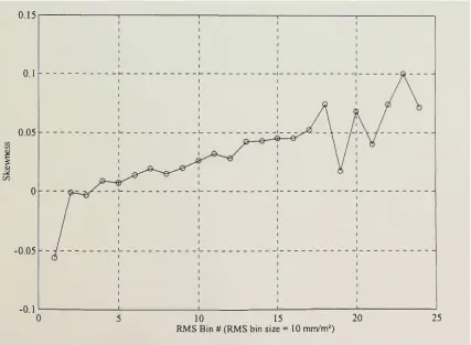
Figure 6.13. Skewness as a function of RMS bin number 74

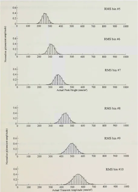
Figure 6.14. Transient ampUtude PDF corresponding to RMS bin #5 to # 10 (bars)

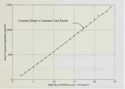
together with equivalent Gaussian (lines) 76 Figure 6.15, Relation between transient amplitude fi and corresponding RMS bin # 77

Figure 6,16. Relation between transient amplitude CT and RMS bin # 78

Figure 6.17. (a) skewness and (b) kurtosis of transient amphtude PDF's for all

RMS bin # 79 Figure 6.18. Stationary RMS distribution for road 25103b 80

Figure 6.19. Transient amplitude distribution for road 25103b 80

Figure 6.20. Stationary RMS distribution for road 55051 a 81

Figure 6.21. Transient amplitude distribution for road 5505la 81

Figure 6.22. Stationary RMS distribution for road 25401b 82

Figure 6.23. Transient amplitude distribution for road 25401b 82

and (b) RMS distributions 84 Figure 7.1. Reconstruction of a section of road profile 86

Figure 7.2. Schematic of road transport vibration simulation with road surface

command signal and physical vehicle suspension model 88 Figure 7.3, Schematic of road transport vibration simulation with vertical acceleration

command signal and numerical vehicle model. 88 Figure 7.4. Schematic of road transport vibration simulation with vertical acceleration

command signal with compliance of suspension system controller. 89

Figure 7.5. 100 m extract of spatial acceleration, road 55051a, 100 m 91

Figure 7.6. Results from computer software, road 55051a, 100 m (line = RMS history,

dots = transient location and amplitude) 91 Figure 7.7. Transient amplitude distribution (bars = entire road 55051a - 8.33 km,

line = entire 415 km sample) with classification parameters 92 Figure 7.8. Stationary RMS distribution (bars = entire road 55051a - 8.33 km,

line = entire 415 km sample) with classification parameters 92 Figure 7.9. 100 m extract of spatial acceleration, road 25103a, 100 m 93

Figure 7.10, Resuhs from computer software, road 25103a, 100 m (line = RMS history,

dots = transient location and amplitude) 93 Figure 7,11. Transient amplitude distribution (bars = entire road 25103a - 3.26 km,

line = entire 415 km sample) with classification parameters 94 Figure 7.12. Stationary RMS distribution (bars - entire road 25103a - 3.26 km,

line = entire 415 km sample) with classification parameters 94

Figure A.l. Comparison of profilometer to manual survey (Prem, 1988) 103

Figure A.2. Spectral analysis from profilometer (Prem, 1988) 103

Figure B.l. Butterworth filter characteristics 105

Figure C.l. Gaussian distribution (|i = 0, a = 1) 107

Figure C.2. Illustration of (a) skewness and (b) kurtosis (Press et al, 1992) 108

Figure C.3. Rayleigh distribution for peak heights 109

Figure C.5. Cumulative mean versus window size (points) for four different

locations 112 Figure C.6. Cumulative RMS versus window size (points) for four different

locations 113 Figure C.7. 50 m of spatial acceleration for analysis of window overlap

(road 51881a) 114 Figure C.8. Effect of moving RMS for various overlap (ensemble size = 3m) 115

Figure C.9. Effect of ensemble overlap on the moving crest factor estimate (ensemble

size = 3m) 116 Figure C.IO. Use of RMS bin size to identify stationary sections

Table 2.1. Classification of roads (Dodds and Robson, 1973) 23

Table 2.2. Revised classification of roads (Robson, 1979) 24

Table 4.1. Road profile data information 33

Table 4.2. Summary of statistics for ARRB elevation profile data 44

Table 6.1. Nine classification parameters for road profile spatial acceleration 84

Table D.l. Transient amplitude distribution parameters for all roads analysed 119

1. INTRODUCTION

Products are inevitably damaged in transportation and handling if they are not packaged adequately. Mechanical damage to products in transit is attributed to vibrations and shocks experienced in the transportation environment. The inclusion of a packaging system aims to reduce product damage but usually results in an increase to the cost of the product as deficient or excessive product protection through packaging is costly. Insufficient packaging is self evident through the incidence of damage, but the over-packaging of products is not as easily detectable. Available estimates of costs associated with over-packaging are 130 billion European Currency Units (Ostergaard, 1991). Hidden costs associated with shipment of over-packaged products may be 20 times greater than the cost of excessive packaging materials and it has been estimated that a 40% reduction in packaging volume is possible (Ostergaard, 1991).

The last 20 years have seen a dramatic increase in the movement of freight in Australia alone with activity more than doubling (VicRoads, 1995). The use of road transport has become increasingly popular and it is estimated that, by the year 2015, the shipment of products on roads will increase significantly as shown in Figure 1.1.

s

250

200

2 150

s e o H

B

100

50

0

• Road DRail B Air

d

•

L

•"

•

1

1971 1991 2015 Source: National Transport Planning Task force, December, 1994

Austroads (1997) reports the split of domestic freight movement across four principle modes of road, rail, sea and air as 98.5, 95.2, 96.0 and 0.14 billion tonne-kilometres respectively. However, as observed by Silver and Szymkowiak (1979) and American President Companies (1986), road vehicles produce the highest vibration levels of all three transport modes. Consequently, the ability to design optimum protective packaging for transportation will become even more important than it is today. It will no longer be sufficient to design packaging systems based solely on the minimisation of damage to the product it encases. The influence of global environmental problems will force packaging engineers to arrive at optimum packaging configurations with substantial consideration given to minimising the use of packaging material.

Ideally, optimum package configurations should be designed and developed in conjunction with the product itself to minimise packaging material whilst ensuring the safety of the product. In practice however, package configurations are determined after product development has been completed, which demands that these configurations are validated. This is often achieved through empirical field testing methods which subjects packaged products to the actual transportation environment. If damage occurs to the package or product during field testing, the package is re-designed and tested again until a satisfactory, but not necessarily optimum, design is determined. Although field testing ensures that product-packaging systems are subjected to actual transportation hazards, it is useful only to identify cases of under-packaging. Once a package design is shown to protect a product sufficiently, the reduction of package materials is discouraged due to the cost and time associated with further testing.

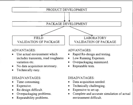
enables over-packaging to be minimised. Advantages and disadvantages of field and laboratory testing are outlined in Figure 1.2.

PRODUCT DEVELOPMENT

PACKAGE DEVELOPMENT

FIELD

VALIDATION OF PACKAGE

ADVANTAGES:

• Use actual environment which includes transients, road roughness variation etc.

• No data acquisition necessary. • Technically easy.

LABORATORY VALIDATION OF PACKAGE

ADVANTAGES:

• Rapid Re-design and testing. • Low Running Expenses. • Overpackaging minimised. • Repeatable tests.

DISADVANTAGES: DISADVATAGES: • Time consuming. • Data acquisition needed.

• Expensive. • Technically challenging. • Re-design difficult. • Expensive to set up.

• Overpackaging problems. • Complete and accurate simulation of actual • Repeatability problems. environment difficult.

Figure 1,2. Schematic for package development and testing

and shocks simultaneously. Parameters commonly used to describe the road transportation environment hazards, such as drop heights, shock levels and vibration levels, have been utilised as the basis for laboratory package performance testing. Testing procedures should aim at simulating the combined effects of all transportation hazards collectively rather than freating them as separate phenomena. Recent attempts made at developing standard laboratory testing procedures in accordance with this concept are discussed in the following chapter. There are standard methodologies in place for the laboratory evaluation of package performance which have major shortcomings. This is a direct result of complications encountered with the accurate characterisation of vehicle vibrations.

2. LITERATURE REVIEW

This chapter covers three main areas of hterature examination. Firstly, existing laboratory techniques for package evaluation formulated by major standard organisations is reviewed. This is followed by a review of techniques used to characterise vehicle vibrations during road transport. Thirdly, methodologies for the analysis of road surfaces, with respect to vehicle-road interactions, are critically investigated.

2.1 REVIEW OF STANDARD LABORATORY PACKAGE EVALUATION

TECHNIQUES

The evaluation of package performance testing in the laboratory is sanctioned by standard organisations world wide. The major organisations involved are International Organisation for Standardisation (ISO), Ausfralian Standards (AS) and American Society of Testing and Materials (ASTM). The development of standard methodologies has been specific so that miss-interpretation of results is minimised. A consequence of this is that the prescribed testing levels are often too high and result in the over-packaging of products. Testing levels prescribed in standard procedures are not always representative of the actual environment.

In 1980, the ISO approved ISO 4180 'Complete, filled transport packages - General

Rules for Compilation of Performance Schedules'. The AS 2584 with the same title is

technically identical. The ASTM recognised the open ended approach of ISO 4180 and the need for development of test methods that reflect the conditions that products experience in normal shipment. The ASTM implemented ISO 4180 as ASTM 4169

'Standard Practice for Performance Testing of Shipping Containers and Systems'. This

vibration can be achieved with the use of procedures outlined in ASTM D 999

'Standard methods for vibration testing of shipping containers'. The ability of a

shipping unit (package and product) to withstand damage caused by vertical vibrations of transport vehicles is assessed by method B - Single container resonance test or method C - Palletised load, unitised load or vertical stack resonance test. A similar procedure is incorporated in ASTM D 3580 'Standard test methods of vibration

(vertical sinusoidal motion) test of products'.

These procedures all consist of two main parts: establishing the resonant frequencies of the packaging system and performing a resonance (sine) dwell endurance test at specific resonant frequencies for a specified length of time or until damage occurs. According to ASTM D 999, system resonances are identified by generating a constant level acceleration sinusoid with variable (sweeping) frequency at the surface on which the product is mounted while constantly monitoring the response acceleration.

The continuous type of deterministic excitation that the ASTM D 999 standard subjects a test package to leads to the possibility of over-packaging as it is unlikely that resonant frequencies are sustained for great lengths of time in an actual transport environment. Further, it is rare that actual excitations are deterministic (harmonic) in nature. ASTM D 999 is an example of'worst case' package performance testing (Sek et al, 1997).

Since shipping containers are exposed to complicated dynamic stresses in the distribution environment, the approximation of product damage, or lack of it, is only possible by subjecting a test package to vibrations which emulates the unpredictable (random) actual environment. As package resonances are excited simultaneously, the resonant build up is less intense than those induced during the resonant dwell or sine sweep methods, and unrealistic damage to test specimen is minimised.

The now commonly used method for experimentally evaluating the effectiveness of packaging systems subjected to random vibrations is outlined in ASTM D 4728-95

standard can be used to assess the ruggedness and performance of shipping units subjected to random vibrations representative of three common modes of transport: road, rail and air. The ASTM D 4728 standard is based on the conjecture that more accurate representation of the common modes of transport is achieved by reproducing a random signal in the laboratory based on its spectral characteristics. Test specimens are placed on a shaker system with the command signal represented by the Power Spectral Density (PSD) estimate of the transport environment. Recommended for use by the standard, transportation PSD's are shown in Figure 2.1 which represent the linear average of a large number of PSD's obtained experimentally over a long period of time.

10"

10'

J5I0''

Q

a.

10

. 1 . . . r 1

•

' 1 ' ' .

Truck Rail

Air

: / / \ ^ :

• / / \ \

/

\

1

10 10 10^

Frequency (Hz)

Figure 2,1. Commercial transport random vibration spectra summary, ASTM D4728-95

lost:

G^ = G , ( / ) * G : ( / ) = R e ( G ^ ) (2-1)

where:

GAA ^ Folded Power Spectrum of GfSf)

Although the instantaneous complex spectrum of a signal contains all relevant information for its exact reproduction, the PSD only contains magnitude and frequency information. This implies that the original signal cannot be reproduced. In order to synthesise a random signal from the PSD, usually via the inverse FFT, the phase spectrum is assumed to be random and uniformly distributed between 0 and 27t resulting in a normally (Gaussian) distributed random signal. This simulated signal is utilised as the command signal for actuation of an electro-hydraulic shaker table which emulates the vertical motion of the vehicle tray. The equalisation of the shaker command signal is required to account for the dynamic behaviour of the test specimen and the shaker to produce the appropriate vibration at the table. ASTM D 4728 recommends the use of the closed loop automatic equalisation method whereby the generated demand signal is controlled by a Random Vibration Controller (RVC) which automatically compensates for the shaker-payload system transfer function to produce the appropriate input signal as shown in Figure 2.2.

DEMAND PROFILE

Random Vibration Controller

EQUALISE RANDOM PHASE

INVERSE FFT

FFT

FROM TABLE

i*-When reproducing random signals from a PSD coupled with a uniformly distributed random phase spectrum, the resulting signal amplitudes will, by definition, be

• 2

characterised by the Gaussian distribution with the (RMS) equivalent to the integral of the PSD. Furthermore, the random signal will be stationary; namely the RMS level of the signal and its frequency content remain constant over time and the signal is free of transients (crest factor » 3.0). Since all modes of transport are characterised, to some extent, by significant fluctuations in vibration level and contain transient events, a synthesised acceleration signal based on a single PSD is not fully adequate for simulation of the transport environment in the laboratory. In the case of road fransport, fluctuations in vibration levels can be considerable as they are at least a function of road surface profiles and vehicle velocity. The procedures outlined in ASTM D 4728-95 do not account for such variations experienced in the fransportation environment. One major shortcoming of the standard is that it recommends that the PSD's shown in Figure 2.1 be used in the absence of a specified PSD whilst stating that "... these PSD profiles do not purport to accurately describe a specific transportation mode or distribution environment. The user of random vibration must verify accuracy and applicability of any data of this type prior to its use.". The PSD's illustrated in Figure 2.1 are in fact representative of "... average vibration intensities measured under various loading conditions, suspension types, road conditions, weather conditions, travel speed etc." Despite these shortcomings, these PSD's are commonly freated and used as 'standard

PSD's' to simulate the fransport environment in packaging laboratories. The use of

these illustrative PSD's for simulation of the transport environment should be discouraged.

extensive data acquisition and analysis is required in order to obtain a sufficiently large stationary record to simulate the transportation process with stationary random signals from the PSD.

2.2 REVIEW OF VEHICLE VIBRATION CHARACTERISATION

Johnson (1971) analysed vibration levels on a 3-ton general purpose truck by measuring acceleration levels on a number of packages over a variety of terrains. The study was designed to investigate the effect that vehicle load, load distributions, tyre pressure, package design, driving technique and lashing had on the response spectrum generated. The data contained transient events with high crest factors, calculated from the instantaneous peak value divided by the underlying RMS, but were removed to allow analysis of the continuous background vibration signal. An extremely non-Gaussian constituent was exposed in the data. Terrain, truck speed, gross load and package position affected the vehicle vertical acceleration levels. The shock levels transmitted to a package were inversely proportional to the payload and as speed increased, so too did the RMS level of vibration. A faster vehicle speed correlated to a higher number of shock occurrences for a given peak 'g' level. Shocks (y) were shown, by Johnson (1971), to approximate to the pulse distribution model:

where:

A = the frequency/mile of peaks,

k = a constant depending on package weight,

X = pulse peak (g's RMS),

Xi = the lower limit of the distribution of peaks.

Hoppe and Gerok (1976) measured vibration and shock levels on loading trays of various transport vehicles. Random vibrations were found to occur in all vehicles between 2 and 500 Hz, and shocks above 10 g were recorded. In the case of trucks, 68% of vibration amplitudes were below Ig, 27% between 1 g and 2 g, and 4% between 2 g and 3 g. The levels for trailers were higher.

affected the resultant power spectrum by causing a shift in the resonant frequencies. Largest accelerations were observed on empty or partly loaded vehicles due to the decrease in overall mass. Shocks of up to 16 g were recorded on semi trailers and up to 25 g on smaller trailers. An averaged PSD, shown in Figure 2.3, was prescribed by Winne (1977), and proposed for use in general purpose testing.

"b

Q CO 0 .

10-'

10-^

10-^

10"

I0-' c

t ' '

• n

1 1

) 5 10 15

1 1 1

20 25 30 Frequency (Hz)

1

35

1

40 45

•

5 0

Figure 2,3, Recommended tractor-trailer vibration test spectrum (Winne, 1977)

vertical accelerations were non-stationary with a non-Gaussian distribution. Further, the shocks present in the recorded data were not removed for the study.

Singh and Marcondes (1992) displayed the vibration levels in trucks as a function of suspension and payload. Their conclusion was that leaf spring frailers have high vibration levels between 3 and 4 Hz and fiilly loaded frailers have lower vibration levels than partially loaded trailers. Air bag suspension trailers have significantly lower vibration levels compared to leaf spring trailers and the sprung mass bounce frequency was found to be approximately 2 Hz. However, damaged air ride frailers exhibited larger vibration levels than leaf spring trailers indicating a need for regular maintenance. Panel vans exhibit significant vibration levels at higher frequencies and the most severe vibration levels in all cases were recorded at the rear of the frailers, shown in Figure 2.4. However, it is not clear from the study if transient events were removed from the PSD estimate. Pierce et al (1992) found that well functioning air ride suspension produce lower vibration levels than leaf spring suspension.

10"^ 10-^ '^ -3 S10 Q w • . 10" 10-^ 1 . 1 , 1 i_ 1 1 y. "" 2l C L ~ x

-1 r 1 ) 1 1 1 1 L 1 L 1

r \

-1 r i 1 1 1 1 1 1 I 1

1 *—1 1 _ J 4 I I 1 -J L -J

1 1 1

1 1 1 --1 r -I

1 1—1 H 1 1

-~i r n

1 1 1 1 1 1

- D _ r a _

J L 3

Y ~i r 1

-X ' ' '

\ ' — ' y

' \ ' /

1 1 — 1

-I 1 1 1 1 1 1 \ 1

1 1 1

1

J

1

J

~ ~ T ~ ~

-iJi< \ 1 1 1 1 II 1 1 1 1 1 II 1 1 1 1 1 II 1 1 1 1 1 l( f I f 1 ( II 1 1 1 1 1

\ ' ~L

~ \ \ y

-\ ' /

1 1 1

4 4 4 -1 J -1 a, 1 - 4 f 4 4

-4 -4 1 1 1 +

r t r -T -T r T T r

-4 l - H —

z n r

4 4 1 T t r

-1 \ -1 -1 T \ T

] ' Y '

1 1 1 1 1 1 1 1 1

4

-L .

4

(

-L .

h

r

-- r • - r •

4

-1

- r •

1

- J - H

1

r

-\ i

\ i

\ [

0° 10' 1 Frequency (Hz)

0^

AAR (1991), Singh and Marcondes (1992), Pierce et al (1992) and tiie ASTM D4728 standard indicates that an experimentally based PSD spectnim is insufficient for the specific description of the vehicle vibration levels of a loading fray. Vehicle response is shown to be a non-stationary, non-Gaussian process which is influenced by the road type, vehicle characteristics and payload. As a result, the response PSD's reported by various researchers can never be identical imless all the pertinent influences are retained constant. This fact often leads to a variation in laboratory testing levels and package designs.

The variation in laboratory test levels derived from actual field data was reviewed by Richards (1990) who investigated four common approaches, namely, the PSD, peak hold PSD, the so called Sandia and Cranfield approach. Richards (1990) shows that measured acceleration amplitudes increase significantly with vehicle speed which results in time varying amplitudes, shown in Figure 2.5.

0.7

0.6

)0.5

iO.4

;0.3

^ 0 . 2

0.1

J

ST

i^m^

1 yn 1 **

1 '^fVjK

y(*

J

10 20 30 40

Vehicle speed (mph)

50 60

In addition, the data contained both transient and continuous steady vibration level characteristics, with the transients difficult to isolate and remove due to their irregular occurrence and amplitude. Richards (1990) discussed the four mentioned acceleration data analysis procedures in detail to outline their advantages and disadvantages.

The traditional PSD approach reviewed by Richards (1990) (as employed by ASTM D 4728), is implemented extensively because of its simplicity. He identified that this method cannot cope with time variant data typically caused by vehicle speed variations and fransients. Richards (1990) showed that, by utilising peak-hold PSD, an indication of the non-stationary nature of the data may be provided. This method uses the maximum PSD values over each spectral band for the entire record and is used to augment the traditional PSD method to enhance results. However, the statistical confidence in the peak hold values vary from the confidence of traditional, averaged PSD values and can produce exfremely conservative test levels with a low probabilities of occurrence, leading to overpackaging.

accepted method of deriving test severities from measured field data experiments. Test results vary throughout the investigated methodologies and there is a need for the introduction of an absolute test method.

The derivation of environment description and test severity from measured data was discussed in depth by Charles (1993). The non-stationary component of vehicle response was shown to be a function of vehicle speed. The analysed data contained prominent non-Gaussian characteristics shown with the use of amplitude probability density fimction (PDF) estimates plotted on semi log versus normalised signed amplitude scales. Further, Charles (1993) found that up to double the vibration severity can be introduced by running vehicles with reduced tyre pressure. He established that any environment description should include frequency response, amplitude probability and time histories of transient events. The analysis procedure used by Charles (1993) is summarised as follows:

• The data is checked for stationarity of RMS and stationary sections used for PSD estimation.

• Transients are identified from time histograms for subsequent capture and determination of shock specfra.

• Variation in vehicle speed is represented on waterfall plots to determine speed dependant peaks.

the averaged PSD approach alone was not adequate to describe and reproduce a transportation environment where non-stationary components were typical.

The traditional simulation method, based on the vehicle response PSD, was revised by Nordstrom et al (1986) who designed an enhanced physical simulation technique for vehicle vibrations based on computer simulation to include fransients and multi directional vibration. Test data was analysed in terms of its vibration specfra and transients, which were freated separately, whilst allowing for large volumes of data to be compressed. They appreciated that vehicle acceleration levels exhibit distinct non-Gaussian and non-stationary characteristics. They propose that, to simulate the transportation environment in the laboratory, a synthesised steady state signal based on the measured acceleration PSD be seeded with pre-recorded transient events. Although the method proposed by Nordstrom et al (1986) is an improvement on previous simulation techniques, which rely solely on the PSD description of the transportation environment, there is still the need for extensive data acquisition due to the number of variables that are not retained constant.

"^^^^^^^^^^^ ' ^ ^ ^ ^ ^'hT;^/^/^^''^^^

Figure 2.6, Suspension compliance with multi-layered loads (Schoori and Holt, 1982)

So far, the research into the description of the fransport environment has cenfred around the spectral description of vehicle response measurements for its complete description. As the simulation of these acceleration levels in the laboratory requires that assumptions be made about the statistics of the process, simulation is inadequate.

Rouillard et al (1996) and Sek (1995) proposed a novel method for simulating the transport environment with the use of road profiles. Vehicle vertical acceleration was replaced by the road surface elevation PSD estimate as the fundamental excitation parameter. The system also includes vehicle models. A schematic of the experimental set up used to verify the procedure is presented in Figure 2.7 in which a road profile was used as the command signal for an electro-hydraulic shaker to actuate a physical half-car.

Successful implementation of this method has distinct advantages over transport environment simulation based on vehicle tray acceleration. Stationary road profile signals could be generated from spectral and statistical parameters derived from the road profile analysis using fraditional techniques. Suitable mechanical devices can be designed to represent the dynamic behaviour of typical road fransport vehicles as well as provide compliance during impact in laboratory simulations. Vehicle speed could be accounted for by a shift in the road elevation PSD along the spatial frequency axis (Newland, 1993 - p 199) as given by:

G,(/) = -G/« = A

(2-3)

where:

V = vehicle transversal velocity, n = spatial frequency,

f = frequency,

RANDOM VTBRATIOH CONTKOLLCR

DEMAND PROFlUa

FFT

EQUAUSE - RAKDOMtSE - IN VERSE FFT

POWER AMPUriCR

LEAD WEICflTS

AMPUriER A %.

— < 3 — z ^

I

PtVOT 5i

SHAKER

JUT <

V '

CIIAROE AMPUFIERS

D T 2 0 0 5 DATA COMPUTER ACQUISmON BOARD

Figure 2,7, Experimental set up from Rouillard et al, 1996

Figure 2.8. Demand and measured elevation PSD (Rouillard et al 1996), speed = 30m/s

2.3 REVIEW OF ROAD PROFILE ANALYSIS TECHNIQUES FOR ROAD-VEinCLE INTERACTIONS

The idea for laboratory testing of vehicle components with the use of road surface simulation was first proposed by Dodds and Robson (1972). A comparison of simulated road profile testing was made against field prototype testing and limitations associated with field testing led to the formulation of road specfra preliminary assumptions for its analysis.

The road surface can be considered a two dimensional random surface and description of such a surface requires elaborate statistical parameters to describe it completely. A vehicle traversing this road surface is subjected to displacements inputs at each wheel, and thus any simplification of the road surface description should account for these direct inputs as well as for correlations between these inputs. Early descriptions of road surfaces considered them as two separate, uncorrelated tracks, that is the left and right track only. Cross correlations between tracks, affecting roll characteristics of a vehicle, were neglected. This did not provide an adequate description for vehicle simulation since it assumed the transverse slope to be uniform at each longitudinal position.

Dodds and Robson (1973) described the road surface as a function of two variables, the longitudinal coordinate x and fransversal coordinate y, by considering the road as a homogeneous, isotropic random process having a Gaussian distribution, provided that occasional irregularities such as pot holes were removed and treated separately. This allowed cross correlations, or cross spectra, to be included in analysis procedures.

From a knowledge of the autocorrelation function, or power spectrum, for a single frack in the x direction, the cross correlation (or cross spectrum) could be estimated from a knowledge of the vehicle geometry. The fimction, y(n) = Sx(n)/SD(n), defined by Dodds and Robson (1973), reinforced practical considerations as the coherence, y (n), approaches unity for small spatial frequency and approaches zero for large spatial frequency. This implies that the admissible range of spatial frequency extend through 0 < n < 00 and since the phase between the two signals is zero, it also implies that the cross spectrum is real.

Verification of these assumptions allowed for a multi-frack response to be obtained from a single track PSD estimate, knowledge of traversal velocity, and dynamic properties of the vehicle.

The shape of the log PSD versus log spatial frequency estimate was found to be independent of road type but a function of the RMS level. A new road classification system based on a single track PSD function was proposed:

S{n) =

S{n,)

s{no)

— ,n<n^

^ „ ^ - -

\nj

,n>n^

where

n = spatial frequency

S(n) = elevation spectral density estimate (m /cycle) w = roughness parameters

UQ = discontinuity spatial frequency = (7i/2 m")

Table 2,1, Classification of roads (Dodds and Robson, 1973) Road Class Motorway Principal Road Minor Road Condition Very Good Good Very Good Good Average Poor Average Poor Very Poor S(n„) (xlO"*')m^/cycle 2-8 8-32 2-8 8-32 32-128 128-512 32-128 128-512 512-2048 wl Mean 1.945 2.05 2.28 Standard Deviation 0.464 0.487 0.534 w2 Mean 1.360 1.440 1.428 Standard Deviation 0.221 0.266 0.263

The model proposed by Dodds and Robson (1973) could not be fully validated because of the lack of real road profile data. It is understandable that subsequent attention has been focussed at vahdating these initial assumptions. Kamash and Robson (1977, 1978) examined the implications and restrictions that this assumption imposed on the admissible range of the subsequent specfra generated.

Robson (1979) further investigated this isotropic model and revised the initial model proposed by Dodds and Robson (1973). The range of spatial frequency considered was restricted to Ug < n < % and made no assumption about the behaviour of the spectra outside of this specified range given by:

S{n)=

c{nj-''' , 0 < | « | < « „

c\n\ , n^ <|«|<nj

0 ,n. >\n\

(2-5)

where:

w = 2.5.

Road Class Motorway Principal Road

Minor Road

Range (x 10"* m^/cycle) 3 - 5 0

3-800 50 - 3000

' c ' (X 10° m^/cycle) 10

50 500

Clossilicatjon by (SO 1110'

11 Iff*

0.10 100 SpotKA Irtqucncy l e y c u / f n )

10 0 0

lOOO _{n o 1.0}

Wavcltnqih <m)

Figure 2,9. Classification of roads by ISO (1982)

Cebon and Newland (1983) further developed the isotropic assumption for roads and proposed to digitally simulate the complete road surface from a single track profile using two-dimensional FFT techniques. Procedures were presented for the digital simulation of heights profiles of a number of correlated parallel tracks and also of entire two dimensional surfaces. Profiles of a number of correlated fracks were generated by the one-dimensional Fourier transform but two-dimensional Fourier transforms are required to generate a fully isofropic surface. Heath (1987a) introduced formulae which involved single integration and subsequent closed form solutions of the cross spectra:

S^{n)= lS'^{n,)J,{2mc^n',-n').dn

where

which implies that the cross spectrum at a particular wavelength is independent of the single track spectrum at a lower spatial frequency. Therefore, the calculation of the cross spectrum requires a measured single frack spectrum of a considerably larger spatial frequency bandwidth. Heath (1987b) assessed the accuracy of the isofropic road roughness assumption using spectral techniques on real road data. He found that spectral analysis supported a hypothesis of real cross specfra between fracks, consistent with the isotropic assumption. Coherences (S^ (n) / Sp (n)) calculated via isofropy agreed well with experimentally determined coherences for asphaltic pavements, but over-predicted measured values for spatial frequency below 0.1 m"'.

With a further modification to the basic isofropic model. Heath (1989) was able to increase the range of spatial frequency in which the experimental and calculated values were in close agreement. These improvements meant that increasingly accurate cross spectra could be generated from knowledge of single track spectra and vehicle dimensions, which reinforced the Dodds and Robson (1973) proposition that road surface classification could be based on a single track profile specfra.

Heath (1989) demonstrated a means of synthesising a single track road profile using the Fourier transform technique in which a spectral array of randomised phase is used in conjunction with the single track specfra to produce, by definition, a Gaussian signal, similar to the method employed by Rouillard et al (1996). However, this specifies that analysis and simulation is limited to the first and second order moments of road roughness statistics.

Road profile analysis and simulations found in literature is predominantly based on a Gaussian distribution assumption and thus is limited to the first and second order statistical moments. Road data analysed by Heath (1988) and Rouillard et al (1996) was shown to have a substantial non-Gaussian component. Rouillard et al (1996) used higher order statistical moments, such as kurtosis and skewness, as an indication of the degree of non-Gaussianity. They also demonsfrated the independence of the road elevation spectral shape to road type, but the data was shown to be non-stationary. Further, calculated crest factors showed the significance of transient events in the road profile but statistical analysis techniques (PDF) of the road profile elevation itself failed to locate these events due to the large amplitude of the low spatial frequency.

The extensive analysis of road profiles relies on their accurate measurement. The research conducted by Dodds and Robson (1973), Cebon and Newland (1983) and Heath (1988) shows that once single track profiles are accurately measured, analysed and characterised, complete surfaces can be generated based on the isotropic model.

2.3.1 Measurement of road surface profiles

Road roughness has traditionally been collected and analysed for the purpose of road maintenance. This has proven important in areas such as road pavement performance and determination of road user costs. Numerous devices have been created to record 'road profile roughness' but they can be classified into two main categories:

• Response Type Road Roughness Measurement Systems (RTRRMS), • Road profilometers.

2,3.1,1 Response type road roughness measuring systems (RTRRMS)

systems induced by fraversing the road surface. A typical arrangement, used in the Bureau of Public Roads (BPR) Roughometer, is shown in Figure 2.10. It is a single wheeled trailer with a one way clutch mechanism, or integrator, to record the motion of its suspension. The roughness is determined by cumulative displacement of suspension stroke per unit distance.

The results obtained from RTRRMS are inevitably influenced by the properties of the host vehicle/trailer. Even with careful calibration and standardisation, the roughness measurements are not stable with time or fransportable to other systems.

RTRRMS allow a repeatable road roughness profile to be obtained at highway speeds and thus they have proved popular as a means of indicating general road surface condition. This type of measurement system is not suitable for detailed road profile analysis. To provide an accurate description of the road profile elevation, actual longitudinal profile elevation is required.

2.3.1.2 Measurement of longitudinal profile

Static methods of profile measurement include: • Staff and level survey,

• Transport and Roads Research Laboratory (TRRL) beam.

profile measuring systems to acquire road data at highway speeds. The Australian Roads Research Board (ARRB) have designed and implemented a laser based profilometer that records actual road profile at highway speeds. The vertical measurement resolution of this system is 0.2 mm and the spatial resolution is approximately 50 mm (Prem, 1987 or see Appendix A). The acquisition method is suitable for the purpose of detailed road profile analysis needed in this thesis.

2.3.2 The international roughness index (IRI)

The World Bank initiated a project to calibrate and standardise roughness measurements and provide a means of correlation between the various measuring systems. The project resulted in the introduction of the International Roughness Index (IRI). The IRI is a standardised version of the RTRRMS readings and provides a methodology to compare the readings from different RTRRMS which are invariably a function of the host vehicle suspension characteristics. Unfortunately, this methodology renders the IRI insufficient for detailed road profile analysis of short wavelength variation and transients.

Gain for Profile Slope |H(v)|

2.0

1.5

1.0

0.5

-0

0.01 0.1 1 10 Wave Number (cycles/m)

Figure 2.11, Spatial frequency response of quarter-car model

IRI provides a suitable methodology for comparison between various RTRRMS readings as well as road profilometer acquisition systems. However, due to the post-processing involved, an absolute road profile cannot be obtained. The IRI does not take advantage of the information attainable from high speed laser profilometers which gives absolute road profile. Therefore, the use of IRI is not suitable for accurate road profile analysis and may become redundant in the future.

An attempt has been made by Marcondes (1990) to relate the IRI to vehicle tray PSD. The study aimed at development of a procedure to predict vehicle PSD as a function of IRI, pavement roughness, vehicle dynamics and speed. A quarter car simulation was used to compute IRI and specfral analysis used for pavement elevation and truck acceleration.

The literature review can be summarised as follows:

• Package performance testing aims at reproducing loading environments in the laboratory, but relevance to actual envfronments vary greatly.

• The simulation of the random transport environment has centred around the description of vehicle vertical accelerations.

• The ASTM D-4728-95 specifies a methodology to simulate random vibration test levels, prescribes recommended PSD's, and outlines the procedure for laboratory simulation. However:

• The level of acceleration experienced by a vehicle has been shown to be a function of five main variables, namely road surface type, suspension characteristics, vehicle speed and payload type and distribution.

• The recommended PSD levels are not indicative of the real transport environment.

• In general, laboratory simulation of the vehicle vibrations based on PSD's produce, by definition, a stationary, Gaussian signal which contain no transient data. This produces vibration levels which vary greatly from the levels obtained in field measurements.

• In order to account for variation in the parameters affecting the vehicle vibrations, much data must be collected for each unique combination of road, vehicle and load.

• The Amplitude Probability Density (APD) of acceleration data has shown that non-stationary and non-Gaussian characteristics cannot be neglected. Recent techniques include these properties for laboratory simulation, but not in a quantifiable manner. • Differences between mechanical compliance of the vehicle suspension and shaker

• The current method of using acceleration response PSD for simulation is inadequate. A method has been outlined which will improve laboratory simulation, but relies on accurate road profile and vehicle characteristic descriptions. This description must account for variations in road surfaces (non-stationarities) as well as irregular, but damaging transient events (non-Gaussian).

• Typical road surfaces have been measured and classified in terms of their spatial PSD only. The characteristic slope of the elevation PSD seems to be independent of the road surface but a function of the RMS (roughness) value of the road.

• No attempt has been made to classify and include transient events or investigate the non-Gaussian characteristic of the road profile elevation data.

• Road surfaces can be determined from single track and cross spectra. Thus, single track description is a sufficient representation of the total road surface.

• RTRRMS values are not an indication of the road profile elevation and can be used only as a guideline for road condition.

• Road profile data can be acquired by laser profilometers at highway speeds with accuracy and resolution suitable for detailed road profile analysis.

• The IRI is not suitable for accurate road profile elevation analysis, when considering short wavelength variations and transients.

• The road profile elevation is, in general, non-Gaussian and non-stationary.

• The use of the road profile (IRI) to predict the acceleration of truck trays has been attempted but with limited success.

• Road profile data has not been used as a control parameter for package performance evaluation.

3.1 GENERAL AIMS

The overall aim of this project is to develop a universal road profile analysis and classification strategy for discretely sampled road data to represent all road profiles. This project is based on the premise that road profile data, coupled with comprehensive vehicle suspension models (physical or numerical), can be used to simulate a wide range of road transportation environments for package performance evaluation and optimisation.

3.2 SPECIFIC AIMS

The specific aims of this thesis are to:

• Comprehensively investigate characteristics of discretely sampled, single track road profile data in both the amplitude and frequency domains.

• Develop an analysis methodology for road profile data to characterise their non-stationary, non-Gaussian and transient properties.

4. FUNDAMENTAL CHARACTERISTICS OF ROAD PROFILES

The analysis of road surface profiles for the purpose of devising a universal classification strategy, for the majority of road types, initially requfres a large sample of road profile data representative of a wide range of road surfaces. These prototype road data can be used to establish the fundamental statistical and specfral characteristics of roads, in general, as well as to validate the infroduction of statistical classification parameters.

Actual data used in this project is a subset of over 20,000 km of Victorian (Ausfralia) road profile data measured with the ARRB laser profilometer (see Appendix A). Twenty one road sections, totalling approximately 415 km, were selected to represent a wide range of bituminous sealed roads, based on the measured NAASRA roughness (NAASRA, 1981). Information on these 21 different road sections is shown in Table

4-1.

Table 4-1. Road profile data information Road Name

Princes Highway East Princes Highway East Princes Highway East Princes Highway East Northern Highway Murray Valley Highway Murray Valley Highway South Gippsland Highway South Gippsland Highway South Gippsland Highway South Gippsland Highway

Midland Highway Goulbum Valley Highway

Maroondah Highway Pyrenees Highway Timboon - Port Campbell Rd.

Wiltshire Lane Daylesford - Malmsbury Rd. Bendigo - Maryborough Rd.

Euroa - Mansfield Road Lismore - Skipton Road

Location (Victoria)

Metro S E Metro S E Metro S E Metro S E

N N N E E E E SW N E Metro S E

N SW

w

w

geographical position. The roughness values were computed by the ARRB to classify the condition of a particular road, with lower numbers indicative of smoother roads. Analysis for this study was conducted on the road profile elevation data acquired at the passenger wheel track.

All figures generated in the subsequent chapters are the result of the analysis of the entire 415 km road profile data with the use of MATLAB . Results presented herein are typical of the results obtained from the analysis of the entire 415 km sample.

4.1 P R E L I M I N A R Y ANALYSIS

4000

3000

2000

e 1000

1000

&

-2000

-3000

-4000

; ; ; : (a)

500 1000 1500 2000

Horizontal Distance, x (m)

2500 3000 3500

6000

4000

2000

.2

M

o

-2000

-4000

-6000

(b)

500 1000 1500

Horizontal Distance, x (m)

2000 2500

It can be shown that the expected frequency spectrum of road profiles are large at zero cycles per metre and become small as the spatial frequency increases (wavelength decreases) as shown in Figure 4.2. This can be visuahsed by the large, hill type fluctuations of large wavelengths and low wavelength and amplitude fluctuations of individual gravel particles.

However, when considering the interaction of vehicles with road profiles, only a range of wavelengths are relevant depending on suspension characteristics of vehicles in general, including wheel and tyre properties. Figure 4.2 shows a spatial bandwidth, (UL, lower spatial frequency - n^, upper spatial frequency) within which significant vibration levels can be expected to be generated as a result of road surface irregularities.

* a lUn i CS b u u o. 00 ( 1 '^^ ' ^ 1 N h-i '^'

\ S

\ \ _\ \ \ \ \ \ \ \ \ _\ - \ \ \ \ \ \ -;

Road Vehicle Interactions

^ w

• ^ — ^

• ~ " --^ N S •^ V ^X >. ^ s X V V s

"^ ^ V

^ -- .._ " • •"— ^

1 1 . L I : !

\ _\ \ \ \ ^ _\ \ _\ \ \ \ \ \ \ \ ^ N 1 N 1

; ^ x 1

HL Spatial Frequency n^ QQ

When considering road profiles as the main source of damage for packages during road transit, it is essential that those wavelengths which induce vehicle resonances are included in the analysis. Several researchers (for example, Marcondes (1990), ASTM D4728 (1995), Singh and Marcondes (1992), Pierce et al (1992) and AAR (1991)) document the first vertical resonant frequency of commercial vehicles as typically 3 to 4 Hz. In order to account for all types of road vehicles, road fluctuations wavelengths of up to 33m will be used for the analysis of road profiles in this study. This corresponds to the inclusion of all excitation frequencies greater than at least 1 Hz for a vehicle speed of up to 120 km/h. In the worst case the amplitude of road fluctuations at 33m wavelengths is such that vehicles travelling at speeds not exceeding 120 km/hr will experience negligible acceleration. The raw road profile elevation specfra for two typical roads is shown in Figure 4.3 which demonsfrates that, as expected, the fluctuation amplitude decreases as spatial frequency increases.

The upper spatial frequency limit (n^) will be a function of the road-tyre interface mechanism which, in itself, will provide natural attenuation of small wavelength events. In addition, the maximum spatial frequency of interest is also affected by the resolution of the measurement system. The ARRB laser profilometer is designed with a Nyquist spatial frequency of 9.8 cycle/m which is, by definition, the absolute upper spatial frequency limit. Examination of the spectrum revealed a significant reduction in road fluctuation magnitude at spatial frequencies greater than 5 m" (corresponding to a wavelength of 0.2m) as illustrated in Figure 4.3.

Spatial Frequency, n, (m' )

Figure 4.3. PSD for two typical roads

^ 30 1 20 c o S 10 > S 0 "S-10 el-'s-20 1 ' 1

1 1

l_ _ _ t 1 r-^ '

1 ^ - ^ • ' V j ' N ^

1

1

: (a)

'r l" ^

1

1

o -30

10 20 30 40 50 60 70 80 90 100

30 20 10 0 10 20 -30

--jrr-\k

I - - / - \ P ^

r —

'

1 1 1

1 1 1 I 1 1 1 1 1 1 1 1

LW^^I / !

\rJi \ / ' \t^

1 1 1

: (b)

1

Y ^ ; i T n r

'

o •

D--a

C 3 •

o a:

10 20 30 40 50 60 Horizontal Distance (m)

70 80 90 100

4.2 S P E C T R A L CHARACTERISTICS

Research resuhs (Dodds and Robson 1973, ISO 1982, Heath 1988, Hegmon, 1993, Xu

et al 1992, Rouillard et al 1994 and Bruscella et al 1997) show that, while the shape of

road spectra is independent of road type, the level of the PSD varies proportional to road roughness. This is manifested as a vertical translation of the road spectra based on the RMS level. Therefore the sole pertinent variable used to describe the spatial PSD of road profiles is the RMS level since RMS is equivalent to the integral of the PSD. Three typical road sections were used to confirm this as shown in Figure 4.5. This phenomenon has the advantage that road roughness can be classified by a single number.

Q on

0. lo'

10^

lo'

lo"

10-'

-^

r

r . \

\ .

' [

"^^

, , 1

^ \

K i n i K DK/IC -1-1-1 r^^ \]A -fit A„ - n O I O I . , , - !

'^^ \

^ ^ 1 V / _ . l ^ , 1 . J . H J - ; . / ^ 1 . 1 1 1 1 , i . V J K J ^ , <_»11 V > . U 1 ^ 1 1 1 1

-••51881a, RMS = 8.58mm, Nd = 41,An = 0.0191m' . :

7'\df\^h R M " ? — 7 9 S m m NH — Q'< A n - f l D l O l m '

!

•

^ \ V i > ^ '

10 _10 Spatial Frequency, n (m" )

Figure 4,5, PSD of three road profile elevations

profiles exhibit non-stationary characteristics and contain transients. Before computing the average PSD, the data should be prepared such that any transient events are removed and that stationary sections be combined and analysed separately. The next section investigates the fundamental amplitude domain characteristics of road profiles.

4.3 AMPLITUDE DOMAIN CHARACTERISTICS

RMS = 3.7 mm skewness = -0.06

kurtosis = 5.8

0 2 Normalised y

Figure 4.6. PDF of road 25103b (bars) with equivalent Gaussian (lines) based on the [i and CT

10 1

-3a

• m A

/

1

L Gaussian

1

1

J

1

+3a

\ 1

\ mi i ; -2

£^10

o

-6 -4 -2 0

Normalised y

1 I 1

-(3a)'

/\y /

1 / 1 1 1

1

I — '

Gaussian

J 1

' — 1 1 1 :

(3a)'

I 1 \ 1

510" 00

o

10

10

-25 -20 -15 -10 -5 0 5 10

Normalised [sign(y)y ]

15 20 25

Figure 4,8, PDF of road 25103b on a semi log scale with equivalent Gaussian

RMS = 8.5 mm - J A ) skewness = -0.34

kurtosis = 8.5

0 2 Normalised y

Figure 4.9, PDF of road 51881a with equivalent Gaussian (a) linear scale (b) semi log scale

0.6

0.5

^ 0 . 4

•="0.3 0.2 0.1 0 -6 1 1 1 L 1 Gaussian r 1 1 1 1 1 1 +

^ /rnlT ll T H 1

III llllllllll

1

RMS = 7.3 skewness =

kurtosis =

. _ — _ - t _ — _ — \ 1

T \ 1

Tlv\ '

[V\ 1

1 mm -0.10 4.3 1 ' 1 (a)

-2 0 2 Normalised y

Table 4-2. Summary of statistics for ARRB elevation profile data Road (File Name) 25101a 25102a 25103a 25103b 25401b 25704a 25704b 25803a 25803b 25803c 25805b 25901a 26404b 27203a 27401a 50381a 51881a 51971a 52001a 55051a 59621a Mean (mm) 0.003 -0.002 -0.003 -0.003 0.008 -0.001 0.000 0.003 0.001 -0.002 0.000 -0.001 0.000 -0.003 -0.002 -0.001 -0.028 -0.002 0.002 -0.001 0.001 RMS (mm) 3.13 2.03 2.65 3.73 7.29 3.45 2.98 4.07 4.84 5.19 5.38 5.23 4.80 7.86 8.47 14.01 8.54 6.93 6.14 9.46 7.89 Skewness -0.04 -0.01 -0.01 -0.06 -0.10 -0.06 -0.27 0.07 -0.14 0.02 -0.16 -0.04 -0.34 -0.14 0.05 3.77 -0.34 -0.17 -0.16 -0.13 -0.07 Kurtosis 7.43 9.74 5.65 5.77 4.33 6.51 11.84 5.73 5.24 6.53 5.12 4.45 15.08 5.19 3.88 128.87 8.50 5.40 15.02 5.59 4.97

standard deviation of the road fluctuation amplitudes. However, there appears to be a

relationship between the kurtosis of the peak distribution and the nominal road

roughness.

P^eak = 0^40mm

<^peak ~ ^-56 mm Kurtosis = 5.37 Skewne^ =_ 0

J22-Normalised a

= 0.89 "=y.3'8

mm

Kurtosis = 8.84

Skewne^= 0 J 4

-— ^ - ^ " " . „ , ^ , f - i

0 2 Normalised a '

Figure 4.12. Peak height distribution with equivalent Gaussian and Rayleigh (road 51881a)

• 1.26 mm Opeak = 8.78 mm Kurtosis = 5.95

Skewne^=-0D4-0 2

Normalised a '