Adaptive bandwidth kernel density estimation for next generation sequencing data

P R O C E E D I N G S

Open Access

Adaptive bandwidth kernel density estimation for

next-generation sequencing data

Parameswaran Ramachandran

, Theodore J Perkins

From

Great Lakes Bioinformatics Conference 2013

Pittsburgh, PA, USA. 14-16 May 2013

Abstract

Background:High-throughput sequencing experiments can be viewed as measuring some sort of a“genomic signal” that may represent a biological event such as the binding of a transcription factor to the genome, locations of chromatin modifications, or even a background or control condition. Numerous algorithms have been

developed to extract different kinds of information from such data. However, there has been very little focus on the reconstruction of the genomic signal itself. Such reconstructions may be useful for a variety of purposes ranging from simple visualization of the signals to sophisticated comparison of different datasets.

Methods:Here, we propose that adaptive-bandwidth kernel density estimators are well-suited for genomic signal reconstructions. This class of estimators is a natural extension of the fixed-bandwidth estimators that have been employed in several existing ChIP-Seq analysis programs.

Results:Using a set of ChIP-Seq datasets from the ENCODE project, we show that adaptive-bandwidth estimators have greater accuracy at signal reconstruction compared to fixed-bandwidth estimators, and that they have significant advantages in terms of visualization as well. For both fixed and adaptive-bandwidth schemes, we demonstrate that smoothing parameters can be set automatically using a held-out set of tuning data. We also carry out a computational complexity analysis of the different schemes and confirm through experimentation that the necessary computations can be readily carried out on a modern workstation without any significant issues.

Introduction

High-throughput sequencing (HTS) has become a cen-tral technology in genome-wide studies of protein-DNA interactions, chromatin-state modifications, gene regula-tion and expression, copy number variaregula-tions, etc. [1,2]. In many cases, such experiments can be viewed abstractly as attempting to measure a“signal” fthat var-ies across the genome. For instance, if the DNA that is sequenced comes from chromatin immunopreciptation (ChIP) of a transcription factor, then the signal f is expected to have the highest amplitude in regions of the genome where the factor binds most strongly. If the sequenced DNA comes from reverse transcription of RNA, then fis expected to have the highest amplitude

in regions of the genome that are most actively tran-scribed. Of course, experience with HTS technologies has shown that such genome-wide signals also reflect other biases or influences–due to, for example, sequen-cing, chromatin accessibility, mappability, etc. [3]. Tech-niques for correcting such biases are beginning to emerge [4,5]. Regardless, highthroughput sequencing continues to generate numerous important insights into the molecular networks that govern the cell.

Various analysis algorithms specialize in extracting bio-logically-relevant information from different types of HTS data. For example, peak-calling algorithms take mapped reads and attempt to identify regions of high enrichment (for review and some comparisons, see [3,6,7]). Some algo-rithms attempt to solve this problem generally, whereas others specialize in identifying punctate transcription-factor binding sites [8,9] or, conversely, broader regional enrichment, as is often seen in histone modification * Correspondence: [email protected]

1

Ottawa Hospital Research Institute, Regenerative Medicine Program, K1H 8L6, Ottawa, Canada

Full list of author information is available at the end of the article

patterns [7,10]. Similarly, a raft of algorithms specializes in estimating gene expression, including the expression of alternative spliceoforms (e.g., [11-14]). While such approaches are clearly valuable, few deal directly with the problem of estimating the genomewide signalf.

Yet, there are many reasons to be interested in such a direct reconstruction. Perhaps the most straightforward is that reconstructingfis useful for visualization in gen-ome browser tracks. Visualization of the signal allows biologists to sanity-check their data, compare different signals at an intuitive level, identify regions of interest, generate hypotheses, and so on [15]. Reconstruction also allows us to manipulate and combine different signals, for example by“subtracting”a background noise/control signal from a treatment signal. Indeed, there is some evidence from the peak-calling literature that true bind-ing and background processes can be separated, leadbind-ing to enhanced signal fidelity [10,16]. We contend that such issues have not been explored in the literature nearly as thoroughly as they should have been, in part because of a lack of focus on the more elementary pro-blem of reconstructing genome-wide signals themselves.

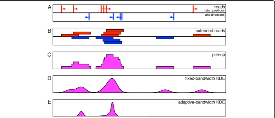
The question then becomes, how can we best recon-struct the genome-wide signals measured by HTS experiments? One simple approach is a read “pileup” map. The details of computing a pile-up depend on whether DNA fragments are sequenced entirely or only partially and, in the latter case, also on whether they are sequenced partially from just one end (resulting in sin-gle-end reads) or from both ends (resulting in paired-end reads). In the case of a single-paired-end dataset, which is probably the most common type of HTS dataset at pre-sent, the sequenced reads are mapped back to the gen-ome to obtain their locations (Figure 1A). Then the positive-and negative-strand reads are either extended to the mean fragment length (Figure 1B) or shifted towards each other by half the mean fragment length. In the for-mer case, the signal profile is built as an aggregation of the intervals representing the fragments (Figure 1C) [16,17]. In the latter case, the simplest way of building a profile is by using a moving histogram. This involves sliding a window of fixed width across the genome and counting the number of reads falling within the window as the window moves forward. Although such histo-grams have been implemented in various versions [8,18-20], in general, histograms are problematic as esti-mators because they are not smooth and the resulting estimates are strongly affected by the choice of histo-gram bin width.

An alternative and more accurate estimator is the

kernel density estimator (KDE), where a kernel (e.g., Gaussian) of a chosen bandwidth (standard deviation) is centered at each sample point (a read), and the kernels are then summed to obtain the density estimate (Figure

1D) [21,22]. Intuitively, high-density regions would cor-respond to tall peaks due to the piling up of closely-spaced kernels. These KDE-based density estimates can be thought of as denoting the probability of finding a read at a given base pair location. QuEST [23], F-Seq [15], and Qeseq [7] apply this method to identify enriched regions in HTS data. Although the density esti-mates obtained by these algorithms are in general smoother and more accurate than those obtained using histograms, the bandwidths of the kernels are fixed and are chosen arbitrarily (QuEST uses 30 bp, Qeseq uses 150 bp, and F-Seq uses an indirect feature-length para-meter to set bandwidth to typically a few thousand bp). The fact that the quality of the density estimates are very much dependent on the choice of the kernel band-width necessitates a more careful and methodical approach to bandwidth selection. In theory, a single optimal bandwidth can be systematically chosen for a given dataset using one of the popular plug-in or cross-validation approaches [24-28]. However, the large gen-ome sizes and the sparsity of HTS data make it a cumbersome process to estimate bandwidth in this man-ner. Even if achieved, a single bandwidth for the entire genome would not usually be sufficient for identifying enriched regions with a high degree of accuracy, owing to the widely varying spatial smoothness of the read distributions. Ideally, small bandwidths work best for high-density regions and large bandwidths work best for low-density regions. If the bandwidth is fixed for the entire genome, then it has to take a compromise value between the two extremes, thus limiting the accuracy of the resulting density estimate. In addition, the estimate would tend to have a large number of spurious local maxima corresponding to individual reads in low-den-sity regions (Figure 1D). Due to these reasons, a fixed-bandwidth KDE is not the best choice for modeling the widely-varying distributions associated with ChIP-Seq or other types of HTS data.

An effective alternative is to use an adaptive scheme that utilizes local data features to dynamically adjust the density estimate to reflect variations in the underlying true density. Adaptive-bandwidth KDE, as the name suggests, achieves this by adapting (or varying) the ker-nel bandwidth according to the local characteristics of the data. Two types of adaptive-bandwidth KDEs have been investigated in the literature. First is the balloon

in higher dimensions, it has serious drawbacks in the univariate and bivariate settings [30,31]. Most impor-tantly, the estimate fails to integrate to one and, in cer-tain situations, has a performance that is worse than that of the fixed-bandwidth KDE.

The second type of adaptive-bandwidth estimator is the

sample-pointestimator, where a bandwidth is selected for each data point instead of the estimation point [32]. The estimate ˆf is then an average of differently-scaled kernels centered at the data points. When the kernel function is a density, fˆitself is a density. This type of estimator has been generally found to be a better performer than the balloon estimator [31,33,34], and is easily adaptable for HTS data. In addition, considering the large genomic sizes that are encountered, the estimate is simple and straightforward to compute since there are only as many kernels as the number of reads in the data. The only caveat, pointed out in [31], is a phenomenon referred to as“non-locality” where the estimate at a certain point can be affected by kernels corresponding to data very far away from it. However, in practice, this would not be an issue because, for the sake of computational feasibility, the kernel tails would have to be truncated after a rea-sonable number of standard deviations. This truncation would typically have no serious consequence as the values involved would be very small.

In this paper, we present an adaptive-bandwidthKDE for modeling the tag distributions of HTS data. The esti-mator automatically adjusts to the smoothness variations

by choosing an appropriate local bandwidth for every read location, thereby leading to a much better estimate of the underlying distribution compared to that obtained using a fixed-bandwidth KDE. To the best of our knowl-edge, adaptive-bandwidth KDEs have not been considered for HTS data before. The method is inspired from the

sample-point estimator [32], but has a number of new features that have been specifically developed to make it suitable for use in HTS data analysis. We consider three possibilities for the choice of the kernel function, namely, the square, triangular, and Gaussian distributions, and compare and evaluate their performance using a number of public datasets. For more detailed discussions on adaptive KDEs in general, the reader is referred to [29-31,33-35] and references therein.

Methods

Datasets

We compare different density estimation approaches on a suite of ten ENCODE single-end ChIP-Seq datasets avail-able through the Gene Expression Omnibus. We down-loaded the data in the form of BAM files, in which reads have already been mapped to positions in the human genome. We chose five datasets describing pulldowns for histone 3 with the following modifications: H3K27ac (GSM733718), H3K27me3 (GSM733748), H3K36me3 (GSM733725), H3K4me1 (GSM733782), and H3K4me2 (GSM733670). The other five datasets describe binding of the following transcription factors: BRCA1 (GSM935377),

CTCF (GSM733672), GTF2F1 (GSM935581), RAD21 (GSM803466), and REST (GSM803365). For the sake of computational convenience, we restricted our attention to estimating the genomic signal on chromosome 1. In pilot studies we conducted, there were no significant dif-ferences in conclusions based on density estimation over the whole genome versus density estimation on just chro-mosome 1. By focusing on chrochro-mosome 1, our computa-tions proceeded much faster. Hence, we first isolated the reads from chromosome 1, removed any duplicate reads, and then shifted positive and negative strand reads towards each other by one half the fragment length, which was estimated using the MaSC approach [5]. We took the starting positions of the resulting reads as data “points” for the purpose of density estimation, and sorted them in ascending order. Each dataset was thus reduced to a sorted list of positionsX= (x1,x2,. ..,xn).

Fixed and adaptive bandwidth kernel density estimators

From a density-estimation perspective, the data X is viewed as being sampled from some unknown distribu-tionf(x) on the genome. The idea is to estimate fusing the sample data. We do this with a kernel density esti-mator, which is of the form

ˆ

Here,xis a query pointat which we want to evaluate our estimate of f,Kis a kernel function, xi is a sample

data point, and hi is thebandwidth associated with xi.

The kernel function K, for example, might be Gaussian in shape, with mean zero and standard deviationhi. The

translated kernel,K(x−xi,hi), would then have meanxi.

In a fixed-bandwidth kernel density estimate, hi is

equal to a constant value h, which may be chosen a priorior dependent somehow on the data. Intuitively, the larger h is, the more aggressively the data is smoothed, because the kernel function becomes broader for largerh. Below, we also experiment with blending fixed-bandwidth estimators with a uniform density. This creates a density of the form fˆ_ε(x) = (1−ε)ˆf(x) +εu(x), whereε Î[0, 1], ˆf(x)is the kernel density estimate of Eqn. 1, and u(x) is a uniform density over the genome. [In fact, because we are concerned with probabilities over integer base pair positions, we should be discussing probability distributionsrather than probabilitydensities. However, in keeping with the traditional terminology of these estimators, we will employ the term ‘density’ throughout.]

In an adaptive-bandwidth kernel density estimator, each hiis allowed to be different. We employ a variant

of the k-nearest neighbor rule to assign the bandwidth

hi. In the statistics literature, there are various schemes

for assigning bandwidths. Perhaps the simplest and the most practical rule is to assign to pointxi a bandwidth hiequal to the absolute distance fromxi to itskth

near-est neighbor [31]. We will call this the KNN1 rule. Intuitively, in regions of sparse data, the kth nearest

neighbor will be far away, and so large bandwidths will be assigned, leading to aggressive smoothing of the sig-nal. In dense regions, on the other hand, thekth nearest

neighbor will be much closer, leading to small band-widths, and thereby an accurate reconstruction of the signal. The choice ofkallows us to indirectly control (to a certain degree) the bandwidth assigned to each point– large k values generally lead to large bandwidths, although the exact bandwidth assigned to each point depends on its proximity to its neighbors.

It turns out that the KNN1 rule has a minor problem which can be awkward in practice. Consider the situa-tion where there are two regions of dense data with a sparse region in between. It may so happen that the bandwidths of all points (at least for some choices ofk) may be set by points within the same dense region. Consequently, no points, including those at the inside edges of the dense regions, would be assigned a large bandwidth, wide enough to cover the span of the sparse region. Therefore, the points in the sparse region may each end up with a probability of zero. If we then evalu-ate a new set of data points on the density estimevalu-ate, and a single point from this set happens to fall in the afore-mentioned sparse region, then the zero probability assigned to this point would result in the joint probabil-ity of the new set of points to be zero–all because of that single point in the sparse region. This “zero pro-blem” is quite common with ChIP-seq datasets, where there are large numbers of very sparse regions.

To circumvent this problem, we propose a variant of KNN1 for assigning bandwidths, which we call KNN2. According to this rule, a pointxiis assigned the same

bandwidth as in the KNN1 rule unless allkof its near-est neighbors are on the same side (left or right). In that case, we instead take the bandwidth to be the distance to the single nearest point in the opposite direction. This rule ensures that the density estimate is nonzero everywhere (except possibly at the extreme ends of the range), thereby avoiding the zero problem.

Kernel functions

that distribution is approximately equal to the band-width parameter. This ensures the greatest comparability of results from different kernel functions in experiments where we vary bandwidths or employ adaptive band-widths. We also take care that each kernel function sums to one. As such, the three kernel functions we consider are

ensure, as a function of bandwidth, that each kernel sums to one.

Results and discussion

Effects of different density estimation schemes in genomic signal reconstruction

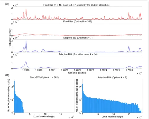
To help visualize the effects of different density estima-tion approaches on real data, we computed fixed- and adaptive-bandwidth Gaussian density estimates based on the Rad21 data in a window of chromosome 1. For fixed-bandwidth estimation, we considered two choices:

h= 16 (close to theh= 15 default used in QuEST), and

h = 362, which we show in the next subsection to be the optimal value according to the probability of held-out tuning data (at least when optimized over integer powers of√2). For adaptive bandwidth, we also consid-ered two choices:k= 7, which is optimal according to a held-out tuning dataset, and k= 14, chosen to increase smoothing.

The results are shown in Figure 2A. The fixed band-width estimate with h= 16 includes many fluctuations across the window. Indeed, in data-sparse regions of the window, each data point (shown by a black mark) pro-duces its own small bump in the curve, just as in our idealized example of Figure 1. Between these bumps, the density estimate is zero–although it is probably reason-able to expect that, if the experiments were repeated, reads may appear at other locations within the region of generally low signal. Still, the density estimate is highest where the most data can be found, and these strong peaks in the curve are readily picked out by the eye. With the larger bandwidth ofh= 362, most fluctuations in the curve are smoothed away, leaving only broad swells where the data is most dense. This, correctly, eliminates the visual distraction of small fluctuations, although it also de-emphasizes the more dense regions

and possible structure within them (such as possible multiple peaks). The adaptive bandwidth estimates elim-inate small fluctuations for both choices ofk, while still strongly emphasizing data-dense regions. The difference between the estimates corresponding tok = 7 andk= 14 has more to do with the fine structure of dense regions–questions such as“is an enriched region a sin-gle peak, or two or three separate peaks?” In the next section, we demonstrate thatk(or h) can be optimized using held-out data in a tuning set. However, such ques-tions of fine structure may also be studied by consider-ing additional information, such as the locations of binding motifs for the factor, or signals in other ChIP-Seq datasets.

To quantitatively demonstrate the qualitative effects described above, we identified all strict local maxima for chromosome 1 in the fixed bandwithh = 362 and the adaptive bandwidthk= 7 curves. The curvefhas a strict

local maximum at positionb iff(b)> f (b−1) andf(b)

> f (b + 1). While some local maxima correspond to regions of high read densities that are biologically signif-icant, such as a transcription-factor binding site, other local maxima correspond to peaks of stand-alone kernel functions corresponding to individual reads that are likely to have no significance. Figure 2B shows grams of the heights of these maxima. From the histo-grams, we see that the adaptive bandwidth estimator produces a much wider range of peak heights resulting from the fact that it strongly emphasizes data-dense regions. It also produces a smaller number of local max-ima (NLM)–a trend that holds for most, though not all, of the datasets we have considered here (see Table 1). Unsurprisingly, we note a generally inverse relationship between the bandwidth h or the number of nearest neighbors k and the number of local maxima in the resulting density estimate. Nevertheless, all density esti-mates have tens of thousands of local maxima, consider-ing that these results correspond only to chromosome 1. Therefore, when computed for the whole genome, the numbers can be expected to be much greater than the expected number ofbona fide binding sites for a tran-scription factor.

Figure 2Effects of different signal-reconstruction approaches. (A) From top to bottom: fixed-bandwidth Gaussian estimators for a portion of the Rad21 data usingh= 16 (close to theh= 15 that is default in the QuEST software) andh= 362 (which appears optimal based on evaluation of held-out tuning data), adaptive-bandwidth Gaussian estimators usingk= 7 (optimal based on held-out tuning data) andk= 14 (double the optimal choice, and intended to obtain more aggressive smoothing). In each plot, the curve shows the reconstructed density. The short black vertical marks indicate the read positions. (B) Histograms of heights of local maxima for fixed-bandwidth Gaussian (h= 362) and adaptive-bandwidth Gaussian (k= 7). Note that the vertical axes are in log scale.

Table 1 Optimized Parameters

Dataset Fixed BW KDE Adaptive BW KDE

Opt.h NLM CPU time (s) Opt.k NLM CPU time (s) (Gau/Tri/Sq)

H3K27ac 1024 40892 395 18 32357 1563 / 653 / 161

H3K27me3 2048 21476 230 16 12291 1513 / 620 / 128

H3K36me3 2048 21052 679 25 19035 2117 / 946 / 217

H3K4me1 1448 28264 240 7 43188 763 / 300 / 74

H3K4me2 724 55799 336 11 41147 934 / 376 / 83

BRCA1 1448 29078 861 24 33822 2158 / 842 / 233

CTCF 512 82386 184 8 53094 685 / 249 / 54

GTF2F1 1024 40399 573 22 37024 1776 / 633 / 148

RAD21 362 111671 158 7 51692 629 / 256 / 61

signal, due, of course, to its well-known smoothing and denoising properties [36].

Adaptive-bandwidth KDE outperforms fixed-bandwidth KDE on held-out data

To more formally assess the accuracy of different den-sity estimation strategies, we randomly divided each dataset into three parts: 50% for training (i.e., creation of the density estimate), 25% for tuning (setting para-meters such as bandwidthhor number of neighborsk), and 25% for testing. We first focus on the results for Rad21, which are largely representative of the other datasets, before presenting a comparison across all ten datasets.

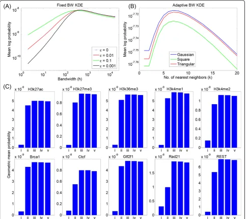
Figure 3A shows the results of several fixed-bandwidth density estimators on the Rad21 dataset: the standard fixed-bandwidth Gaussian kernel estimate (ε= 0), and that same estimate blended with a 10%, 1%, and 0.1% uniform density (ε= 0.1, 0.01, and 0.001, respectively). The vertical axis shows the mean log probability of the tuning data under the density estimate obtained using the training data. The horizontal axis shows the effect of varying the bandwidth. [The mean log probability of the tuning data is equivalent to the logarithm of the geo-metric mean of the tuning data point probabilities. We use the logarithm here for greater visibility of the plots. We employ the mean across tuning points so that differ-ent datasets with differdiffer-ent total numbers of points can be compared directly.]

For theε= 0 case, it is only at the largest tested value of the bandwidth parameter,h = 215 = 32768, that the tuning data has a nonzero probability. For smaller band-widths, some tuning data points are left uncovered by any kernel in the training density. Such points get assigned a zero probability individually and, therefore, the entire tuning set is assigned a zero probability. For a typical, point-binding transcription factor, the peaks in the density may be a few hundred base pairs wide, and therefore smoothing with a kernel bandwidth in the tens of thousands is not ideal. In such situations, then, the vast regions of low signal levels demand a bandwidth inappropriate to the more interesting parts of the signal, and therefore choosing a single bandwidth becomes difficult.

For the ε>0 cases, the uniform density component solves the “zero problem” of tuning points being left uncovered (similar to our previous use of a uniform mixture component in analyzing multi-modal flow cyto-metry data [37]). The tuning data thus has nonzero probability for all choices of bandwidth, and by varying the bandwidth we can choose an appropriate one, as shown in Figure 3A. For this dataset, an appropriate bandwidth appears to be in the range of 500 to 1000 base pairs. We note that the best choice of bandwidth

has some dependence on the ε parameter. Moreover, different choices of εlead to mildly differing probabil-ities of the tuning data if bandwidth is optimized. For all choices of ε, however, we clearly see that too small a bandwidth leads to undersmoothing of the data, as seen by very poor probability of the tuning data. When band-width is too large, oversmoothing results, and the prob-ability of the tuning data also suffers, although this loss is not as severe as that with undersmoothing. For other datasets, we often found that the tuning curves were even flatter for high bandwidths than the Rad21 tuning curve, rendering these datasets relatively resistant to oversmoothing. For the remainder of our analyses, we focus on theε = 0.1 choice. Although the tuning data were slightly less probable with this choice than with smaller values of ε, this choice favored smaller band-widths h, which is preferable for emphasizing regions of true signal density.

Figure 3B shows the results of adaptive-bandwidth density estimators with Gaussian, triangle, and square kernel functions for varying values of the nearest-neigh-bor parameter k. These results are again for the Rad21 dataset, and show the mean log probability of the tuning data under the density estimate obtained from the train-ing data. We have used the KNN2 rule for assigntrain-ing bandwidths. For this dataset, we find that an optimal value of k = 7 can be chosen based on the tuningset probability. Values smaller than this optimal value result in undersmoothing, and larger values result in over-smoothing. However, in absolute terms, the tuning-set probability actually changes very little as a function ofk. The probability using the best value of k (7) is only about 10% higher than under the worst value of k

tested. By way of comparison, better or worse values of the bandwidth parameterhfor the fixed-bandwidth esti-mators in Figure 3A resulted in orders-of-magnitude differences in the tuning-set probability. We also observe that the probability of the tuning data obtained under the adaptive-bandwidth scheme is higher than that obtained under the fixed-bandwidth scheme. Intui-tively, the adaptive-bandwith scheme allows, by design, coverage of sparse data regions without sacrificing accu-racy in high-density regions. The Gaussian and triangle kernels performed very similarly, with the Gaussian being slightly better at all values ofk. The square kernel fared slightly worse, although the difference is small compared to even the small loss that may result from a poor choice of k, let alone the difference observed for fixed-bandwidth density estimators.

fixed-bandwidth Gaussian kernel estimation withε= 0.1 and bandwidthhoptimized on the tuning set, and adap-tive-bandwidth estimation with Gaussian, triangle, and square kernel functions with KNN2 bandwidth selection and optimalk(chosen to maximize tuning-set probabil-ity). We report geometric mean probability of the test data points in the bar charts, while Table shows the optimized bandwidthshor nearest neighbor parameters

k, depending on the method. The results are remarkably consistent across the 10 datasets. Adaptive-bandwidth estimation with Gaussian kernels is uniformly the best performer, followed closely by the triangle and the

square kernels. Thus, by the measure of mean log prob-ability of test data, the Gaussian kernel is consistently best at smoothing (or denoising) the data. Among the two fixed-bandwidth cases, the approach of optimizing bandwidth on a tuning set always leads to improved test-set performance, emphasizing the importance of using a tuning set to optimize algorithm parameters. For many datasets, the fixed (but optimized) bandwidth Gaussian estimator is only about 10% worse than the adaptive-bandwidth schemes, although for some datasets its performance drops to about two-thirds or even one-half of that of the adaptive-bandwidth schemes. The

Figure 3Held-out tuning data analysis. Assessment of (A) fixed and (B) adaptive bandwidth schemes on held-out tuning data from the Rad21 dataset across a range of the bandwidth parameterhand thekth-nearest neighbor parameterk. (C) Comparison of five different approaches on

unoptimized fixed-bandwidth scheme is uniformly the worst, with a test-set probability on average about one-tenth of that of the other schemes.

Kernel function choice influences time and space complexity

Although our analysis shows that the choice of the ker-nel function–Gaussian, square, or triangle–has little influence on tuning or test-set probabilities, the choice does impact the computational resources needed to compute the densities. The final columns of each half of Table show the CPU times, measured in seconds on a SunFire x2250 cluster computing node, for evaluating the full density estimate across chromosome 1 for the three different kernel functions. The Gaussian estimate is always the most expensive to compute, and there are two main reasons for this. First, it has the widest sup-port of all the kernels (10 standard deviations in dia-meter), and it involves evaluation of the exponential function, which is a relatively time-consuming opera-tion. The triangle estimate, with a smaller support and a simple function to evaluate, was typically about 2.5 times faster to compute. The square estimate, with the narrowest support and a constant height (though depen-dent on bandwidth), was roughly 10 times as fast to evaluate as the Gaussian estimate.

In slightly more formal terms, if we have Dtraining data points, Sbase pairs of average kernel support, and a genome of sizeGbase pairs, then we expect O(DS+

G) computations to evaluate a kernel density estimate. TheGterm is for initializing the density to zero every-where, and the DS term is for evaluating each kernel over the base pairs to which it contributes probability mass. Empirically, the linear influences ofDand S are well born out when we plot, for instance, CPU time ver-sus dataset size or mean bandwidth size. Different ker-nel functions affect mainly the slope of the relationship of CPU time toDor S–i.e., they determine the constant inside the big O.

This analysis, however, assumes explicit representation of the density value at every base pair. The square ker-nel density estimate is piecewise constant, comprisingO

(D) pieces–each data point contributes one rise and one fall to the function ˆf(x). Thus, the density can be repre-sented in terms of the start, end, and height of each piece, and can be computed in O(D) time and requires onlyO(D) space (as opposed toO(G) space for a general density over the whole genome). Moreover, such a pie-cewise constant density is readily represented as a BED file, making it convenient for browser viewing. For the triangle kernel function, the density estimate is piece-wise linear withO(D) pieces; this too can be handled in

O(D) time and space, although we know of no browser

file format allowing piecewise linear functions. Given that the triangle kernel has similar computational requirements to the square kernel, and yet an accuracy comparable to the Gaussian kernel, defining a browser file format that allows for piecewise linear functions could be advantageous. Thus, although accuracy points to the Gaussian kernel as the best choice for density estimation, square and triangle kernels have points in their favor regarding computation and browsing convenience.

Conclusions and future work

We have investigated adaptive-bandwidth kernel density estimators for the reconstruction and visualization of genomic signals underlying ChIP-Seq data, with several results. First, we found that adaptive-bandwidth schemes generally outperform fixed-bandwidth schemes in terms of accuracy. In our opinion, adaptive-bandwidth schemes also hold visualization advantages, although we admit this is somewhat subjective. With optimized smoothing parameters, fixed-bandwidth estimators held a slight advantage in terms of computation time, although all estimates can be computed quickly enough that computation time does not seem to be a major concern. Among different kernel functions, we found that all yielded comparable accuracy with some having potential advantages in terms of compact representation and genome browser compatibility. It remains to be investigated whether the increased accuracy of adaptive-bandwidth estimates will translate into improved abil-ities of extracting biological information–for instance, in terms of transcription factor binding sites or peaks, assessment of regions of enrichment for histone marks or, more generally, comparison of different ChIP-Seq signals. Relatedly, our methods may be useful in more accurately decomposing genomic signals into constitu-ent parts, or correcting for differconstitu-ent sources of bias. One way to do this would be to create adaptive-band-width KDE smooths of different possible sources of bias (e.g., local GC content, mappability, etc.), and then use regression, deconvolution, or principal components style anlayses to isolate the true signal of interest. Alterna-tively, one might generalize the adaptive-bandwidth KDE approach to that of conditional density estimation to account for possible biases at the time of signal reconstruction. We leave these questions as topics for future study.

Software implementing adaptive-bandwidth density estimation for ChIP-Seq data is available at http://www. perkinslab.ca/Software.html.

Competing interests

Authors’contributions

PR and TJP conceived the ideas, designed the experiments, and wrote and approved the paper.

Acknowledgements

This work has been supported in part by grants from the Natural Sciences and Engineering Research Council of Canada (NSERC), the Government of Ontario Ministry of Economic Development and Innovation (MEDI), and the Ottawa Hospital Research Institute (OHRI).

This article has been published as part ofBMC ProceedingsVolume 7 Supplement 7, 2013: Proceedings of the Great Lakes Bioinformatics Conference 2013. The full contents of the supplement are available online at http://www.biomedcentral.com/bmcproc/supplements/7/S7.

Declarations

Funding for the publication of this article was provided by the_‘Author Fund in Support of Open Access Publishing’established by the University of Ottawa.

Authors’details

1

Ottawa Hospital Research Institute, Regenerative Medicine Program, K1H 8L6, Ottawa, Canada.2_{University of Ottawa, Department of Biochemistry,}

Microbiology and Immunology, Faculty of Medicine, K1H 8M5, Ottawa, Canada.

Published: 20 December 2013

References

1. Mardis ER:A decade’s perspective on DNA sequencing technology.

Nature2011,470:198-203.

2. Park PJ:ChIP-Seq: Advantages and challenges of a maturing technology.

Nat Rev Genet2009,10:669-680.

3. Pepke S, Wold B, Mortazavi A:Computation for ChIP-Seq and RNA-Seq studies.Nat Methods2009,6:S22-S32.

4. Benjamini Y, Speed TP:Summarizing and correcting the GC content bias in high-throughput sequencing.Nucleic Acids Research2012,40(10):e72. 5. Ramachandran P, Palidwor GA, Porter CJ, Perkins TJ:MaSC:

Mappability-sensitive cross-correlation for estimating mean fragment length of single-end short-read sequencing data.Bioinformatics2013,29(4):444-450. 6. Wilbanks EG, Facciotti MT:Evaluation of algorithm performance in

ChIP-Seq peak detection.PLoS ONE2010,5(7):e11471.

7. Micsinai M, Parisi F, Strino F, Asp P, Dynlacht BD, Kluger Y:Picking ChIP-Seq peak detectors for analyzing chromatin modification experiments.

Nucleic Acids Research2012,40(9):e70.

8. Zhang Y, Liu T, Meyer CA, Eeckhoute J, Johnson DS, Bernstein BE, Nusbaum C, Myers RM, Brown M, Li W, Liu XS:Model-based analysis of ChIP-Seq (MACS).Genome Biol2008,9(9):R137.

9. Narlikar L, Jothi R,et al:ChIP-Seq data analysis: Identification of protein-DNA binding sites with SISSRs peak-finder.Methods Mol Biol2012,

802:305-322.

10. Zang C, Schones D, Zeng C, Cui K, Zhao K, Peng W:A clustering approach for identification of enriched domains from histone modification ChIP-Seq data.Bioinformatics2009,25(15):1952-1958.

11. Anders S, Huber W:Differential expression analysis for sequence count data.Genome Biol2010,11(10):R106.

12. Robinson M, McCarthy D, Smyth G:edgeR: A Bioconductor package for differential expression analysis of digital gene expression data.

Bioinformatics2010,26:139-140.

13. Robinson M, Oshlack A,et al:A scaling normalization method for differential expression analysis of RNA-Seq data.Genome Biol2010,11(3): R25.

14. Trapnell C, Hendrickson D, Sauvageau M, Goff L, Rinn J, Pachter L:

Differential analysis of gene regulation at transcript resolution with RNA-Seq.Nat Biotechnol2013,31:46-53.

15. Boyle AP, Guinney J, Crawford GE, Furey TS:F-seq: A feature density estimator for high-throughput sequence tags.Bioinformatics2008,

24(21):2537-2538.

16. Rozowsky J, Euskirchen G, Auerbach RK, Zhang ZD, Gibson T, Bjornson R, Carriero N, Snyder M, Gerstein MB:Peakseq enables systematic scoring of ChIP-Seq experiments relative to controls.Nat Biotechnol2009,27:66-75.

17. Tuteja G, White P, Schug J, Kaestner KH:Extracting transcription factor targets from ChIP-Seq data.Nucleic Acids Res2009,37(17):e113. 18. Kharchenko PV, Tolstorukov MY, Park PJ:Design and analysis of ChIP-Seq

experiments for DNA-binding proteins.Nat Biotechnol2008,26:1351-1359. 19. Ji H, Jiang H, Ma W, Johnson DS, Myers RM, Wong WH:An integrated

software system for analyzing ChIP-ChIP and ChIP-Seq data.Nat Biotechnol2008,26(11):1293-1300.

20. Jothi R, Cuddapah S, Barski A, Cui K, Zhao K:Genome-wide identification of in vivo protein-DNA binding sites from ChIP-Seq data.Nucleic Acids Res2008,36:5221-5231.

21. Rosenblatt M:Remarks on some nonparametric estimates of a density function.Ann Math Statist1956,27(3):832-837.

22. Parzen E:On estimation of a probability density function and mode.

Ann Math Statist1962,33(3):1065-1076.

23. Valouev A, Johnson DS, Sundquist A, Medina C, Anton E, Batzoglou S, Myers RM, Sidow A:Genome-wide analysis of transcription factor binding sites based on chip-seq data.Nat Methods2008,5(9):829-834.

24. Rudemo M:Empirical choice of histograms and kernel density estimators.Scandinavian Journal of Statistics1982,9(2):65-78. 25. Sheather SJ, Jones MC:A reliable data-based bandwidth selection

method for kernel density estimation.Journal of the Royal Statistical Society, Series B1991,53(3):683-690.

26. Hall P, Marron JS, Park BU:Smoothed crossvalidation.Probability Theory and Related Fields1992,92:1-20.

27. Cao R, Cuevas A, Manteiga WG:A comparative study of several smoothing methods in density estimation.Computational Statistics & Data Analysis1994,17(2):153-176.

28. Jones MC, Marron JS, Sheather SJ:A brief survey of bandwidth selection for density estimation.Journal of the American Statistical Association1996,

91(433):401-407.

29. Loftsgaarden DO, Quesenberry CP:A nonparametric estimate of a multivariate density function.Ann Math Statist1965,36(3):1049-1051. 30. Silverman BW:Density estimation for statistics and data analysis. Monographs

on Statistics and Applied ProbabilityChapman and Hall; 1986.

31. Terrell GR, Scott DW:Variable kernel density estimation.Ann Statist1992,

20(3):1236-1265.

32. Breiman L, Meisel W, Purcell E:Variable kernel estimates of multivariate densities.Technometrics1977,19(2):135-144.

33. Jones MC:Variable kernel density estimates and variable kernel density estimates.Australian Journal of Statistics1990,32(3):361-371.

34. Sain SR, Scott DW:On locally adaptive density estimation.Journal of the American Statistical Association1996,91(436):1525-1534.

35. Botev ZI, Grotowski JF, Kroese DP:Kernel density estimation via diffusion.

Ann Statist2010,38(5):2916-2957.

36. Shapiro LG, Stockman GC:Computer visionPrentice Hall; 2001. 37. Song C, Phenix H, Abedi V, Scott M, Ingalls BP, Kærn M, Perkins TJ:

Estimating the stochastic bifurcation structure of cellular networks.PLoS computational biology2010,6(3):e1000699.

doi:10.1186/1753-6561-7-S7-S7

Cite this article as:Ramachandran and Perkins:Adaptive bandwidth kernel density estimation for next-generation sequencing data.BMC

Proceedings20137(Suppl 7):S7.

Submit your next manuscript to BioMed Central and take full advantage of:

• Convenient online submission

• Thorough peer review

• No space constraints or color figure charges

• Immediate publication on acceptance

• Inclusion in PubMed, CAS, Scopus and Google Scholar

• Research which is freely available for redistribution