P R O C E E D I N G S
Open Access
Finding genes that influence quantitative traits
with tree-based clustering
Ian J Wilson
*, Richard AJ Howey, Darren T Houniet, Mauro Santibanez-Koref
From
Genetic Analysis Workshop 17
Boston, MA, USA. 13-16 October 2010
Abstract
We present a new statistical method to identify genes in which one or more variants influence quantitative traits. We use the Genetic Analysis Workshop 17 (GAW17) data set of unrelated individuals as a test of the method on the raw GAW17 phenotypes and on residuals after fitting linear models to individual-based covariates. By performing appropriate randomization tests, we found many significant results for a proportion of the genes that contain variants that directly contribute to disease but that have an increased type I error for analyses of raw phenotypes. Power calculations show that our methods have the ability to reliably identify a subset of the loci contributing to disease. When we applied our method to derived phenotypes, we removed many false positives, giving appropriate type I error rates at little cost to power. The correlation between genome-wide heterozygosity and the value of the trait Q1 appears to drive much of the type I error in this data set.
Background
Multilocus approaches to associations between variants and traits are likely to be advantageous when rare sin-gle-nucleotide polymorphisms (SNPs), which have an undetectable effect on a trait when considered singly, can explain a large proportion of the genetic variance at a locus when they are taken together [1-3]. Investigators have taken a gene-centric approach to association test-ing ustest-ing, for example, entropy [4], weighted sums [2,3], and distance measures [5] to summarize information across different sites. Our approach uses data-driven tree-based clustering to combine genotypes across mul-tiple loci. The tree structure makes our algorithm an efficient way to search through SNPs that best explain the difference in quantitative trait values. Our tree con-struction method ensures that genotypes that differ by a mutation at a single locus always cluster on the tree and gives an easily interpretable visualization of the SNPs at a locus that affects the trait.
Sevon et al. [6] developed a method, TreeDT, that uses lexical sorting of haplotypes to produce a tree-based test of association. We use the idea of lexical
trees but extend it by using multilocus genotypes and by working with quantitative traits rather than case-control status. The method can be used on haplotypes, but using multilocus genotypes is a natural extension when we are interested in the effects of rare variants, because these variants are unlikely to be present in two copies and phasing of such variants is much more uncertain [7]. We develop this method to work with rare variants by using recoded multilocus genotypes rather than hap-lotypes and by extending the statistics used to look for associations between quantitative traits and the tree structure. Every node on the tree represents a multilo-cus genotype that appears one or more times in the population. Shorter multilocus genotypes are situated at internal nodes of the tree. This method provides a pic-torial summary of the information contained in a region at different genes along the chromosome. The methods presented here are implemented both as a stand-alone program and as an R library [8].
Methods Data preparation
For these analyses we use the unrelated individuals geno-type data from Genetic Analysis Workshop 17 (GAW17); these data consist of 697 individuals genotyped at 22,487
* Correspondence: [email protected]
Institute of Genetic Medicine, Newcastle University, Newcastle NE3 1NB, UK
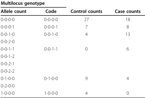
sites. The data generation is detailed by Almasy et al. [9]. For tree analyses, we recode these genotype data as bin-ary multilocus genotypes (BMGs) by coding homozygotes for the common allele as 0 and all other genotypes as 1, so that the BMG of an individual at a gene is a vector of 0’s and 1’s. This recoding is illustrated with example data in Table 1. We perform two sets of analyses: all prelimin-ary work is done on the first phenotype data set, and subsequent power calculations are performed on all 200 data sets.
Principal components and individual variation
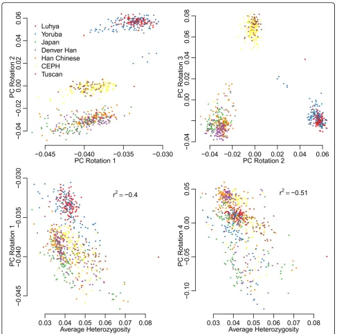
Loadings from principal components analysis (PCA) were calculated for allele counts for all genotype data using standard R functions. Plots of loadings are shown in Figure 1. The first principal component (PC), explain-ing 35% of the variance, does not resemble typical PCA results because it does not produce a separation into the three main population groupings that is seen in other studies with comparable samples [10], whereas rotations 2 and 3 effectively separate the individuals into three groups. Rotations 1 and 4 are more closely related to the overall variation seen in a sample (as measured by average heterozygosity) than to differences between populations, as seen for SNP array data [10].
Derived phenotype data
To incorporate suspected relations between Q1, Q2, Q4, and the other explanatory variables (Age, Smoke, Sex, and PC loadings), we calculate two additional derived phenotypes for each of Q1, Q2, and Q4. We construct the first residual phenotype by fitting the linear model:
Q1=b0+b1(Age)+b2(Smoke)+b3(Sex)+e, (1)
whereε~N(0,s), using backwards stepwise selection on the explanatory variables and using the Bayesian information criterion [11] to decide which variables are retained. After model fitting, we use the standardized residuals as phenotypes. We calculate a second set of derived phenotypes in the same way but with the initial model also containing the first six variable PC loadings, which we label PC1,…, PC6.. All of this model selec-tion is done on phenotype data set 1. We then fit the selected models individually to each of the 200 replicate data sets and use their standardized residuals as pheno-type data. All calculations are performed using standard R functions.
Building trees from genetic data
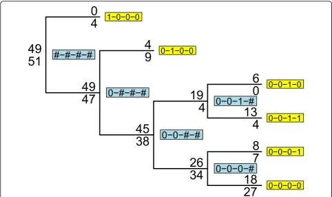
Consider a set of BMGs for a gene (here we could also use haplotypes if we had accurate phasing) as strings of 0’s and 1’s. Put all the individuals at the root of a tree. Now consider the variant positions in that gene one position at a time from left to right or using some other ordering. For the first position, all those samples with a 0 at the position are put on the left branch of the root, and all those with a 1 are put on the right branch. The two leaves of this tree now contain BMGs of length one 1. Now step through all the other variable positions for each leaf. If there is any variation at the current position among the individuals at a leaf, the leaf is split in two, with all individuals with a 0 on the left branch and all individuals with a 1 on the right branch. Repeat for all the variable sites at the gene. After k sites the leaves contain BMGs of length k. This procedure is illu-strated in Figure 2. The multilocus genotypes that map to multilocus genotype codes for our example data are shown in Table 1.
Test statistics
Obtaining a tree test statistic is a two-stage process. First, we require values of partial test statistics defined on the leaves and internal nodes of our tree. A variety of test statistics are available, but we are restricted to those that depend only on values of a trait at a node and its descen-dants. Using information at ancestral nodes or on nodes on other branches of the tree (such as other individuals from the same population) is not possible within this fra-mework. We use the termdisjointhere for a set of nodes in which none of the nodes is the ancestor of another. For further details see Sevon et al. [6].
Although many partial test statistics are possible, we take a simple one, thezscore:
z
x n x
n s i
ij i j
n
i i
=
∑
=1 −, (2)
Table 1 Genotype frequencies for example data set
Multilocus genotype
Allele count Code Control counts Case counts
0-0-0-0 0-0-0-0 27 18
0-0-0-1 0-0-0-1 7 8
0-0-1-0 0-0-1-0 4 13
0-0-2-0
0-0-1-1 0-0-1-1 0 6
0-0-1-2 0-0-2-1 0-0-2-2
0-1-0-0 0-1-0-0 9 4
0-2-0-0
1-0-0-0 1-0-0-0 4 0
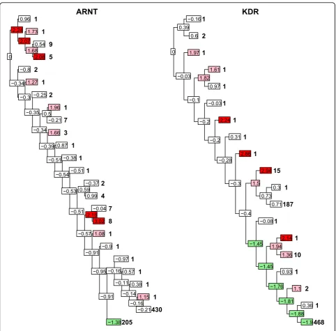
where xij, j = 1, …, ni, are the values of the trait at nodei and x ands are the sample mean and standard deviation, respectively, of the trait over all individuals. Two trees with the respectivez scores at the nodes are shown in Figure 3.
The QTLTree test statistic over the whole tree,Sk, is defined as the maximum value of:
f zi i
k ( )
=
∑
1 , (3)where the summation is over mdisjoint nodes where m≤k, andfis some function. For our analyses, we take:
Sk zi
i k =
=
∑
1
, (4)
that is, f y
( )
= y , but other approaches are possible and implemented in our program. As a side effect of the calculation, we obtain intermediate values for Sj, j= 1,…,k−1. Typically for our tests, we takek= 10. PC Rotation 1
PC Rotation 2
í0.045 í0.040 í0.035 í0.030
í
0.04
í
0.02
0.00
0.02
0.04
0.06
Luhya Yoruba Japan Denver Han Han Chinese CEPH Tuscan
PC Rotation 2
PC Rotation 3
í0.04 í0.02 0.00 0.02 0.04 0.06
í
0.04
0.00
0.02
0.04
0.06
0.08
Average Heterozygosity
PC Rotation 1
0.03 0.04 0.05 0.06 0.07 0.08
í
0.045
í
0.040
í
0.035
í
0.030
r2=í0.4
Average Heterozygosity
PC Rotation 4
0.03 0.04 0.05 0.06 0.07 0.08
í
0.10
í
0.05
0.00
0.05 r2=í0.51
Significance testing
The null distribution ofSkis not available. Because the GAW17 data were sampled from different populations, a straightforward randomization was not appropriate and individuals were randomized within populations; that is, the traits were randomly relabeled within each population so that the mean and standard deviation of the traits stayed the same within populations across replicate permutations. The seven different populations used were Luhya, Yoruba, Japanese, Denver Chinese, Han Chinese, CEPH (European-descended residents of Utah), and Tuscan.
We calculate statistical significance with 106 rando-mized replicates per gene for the phenotype data set. We perform power calculations over multiple data sets using 105 replicate simulations over all 200 data sets. One hundred thousand replicate permutations for all 3,205 genes of a single data set typically takes about 60 minutes, and these calculations are easy to perform in parallel, making them feasible for whole-genome data. The R package QTLTree [8] is available from IJW’s website (http://www.staff.ncl.ac.uk/i.j.wilson).
Results
Model choice derived phenotypes
The backwards model selection results in three additional derived phenotypes: Q1A, the residuals after fitting Age and Smoke; Q1B, the residuals after fitting Age + Smoke + PC1 + PC4; and Q4A, the standardized residuals after fitting a linear model with predictors Age + Sex + Smoke to Q4. No nonconstant terms were kept in models for Q2, and no extra PC terms were kept for Q4.
Analysis of data set 1
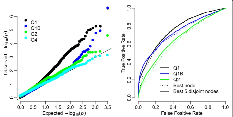
Table 2 gives the genes with the highest significance levels for analyses of the three Q1-related traits and Q2. Although for the uncorrected trait the gene with rank 1 is true, the rest of the top 10 ranked genes are all unre-lated to the trait and are significant after Bonferroni cor-rection (p< 5 × 10⁻⁵). No improvement is seen after correcting for Age and Smoke. Only the derived trait Q1B behaves well. For Q2 there are no false positives after strict Bonferroni correction. Quantile-quantile plots ofp-values from QTLTree tests of Q1, Q2, Q1B, and Q4 are shown in Figure 4. The p-values of phenotype Q4
51
47
38
34
4
49
49
45
26
19
27
7
4
0
9
4
18
8
13
6
4
0
0
í
0
í
0
í
0
0
í
0
í
0
í
1
0
í
0
í
1
í
1
0
í
0
í
1
í
0
0
í
1
í
0
í
0
1
í
0
í
0
í
0
#
í
#
í
#
í
#
0
í
#
í
#
í
#
0
í
0
í
#
í
#
0
í
0
í
0
í
#
0
í
0
í
1
í
#
follow their expectations well, whereas those for Q1 approach acceptability only when using phenotype Q1B, corrected using PC loadings. Results from phenotype Q2 show some deviation from the expected at lowp-values, but these do not seem to be due to true associations from results in Table 2.
Power calculations
Power calculation results are summarized in Figure 4. There is some power to detect true associations at genes influencing traits Q1 and Q2, but not for all genes. Using the derived trait Q1B, which incorporates PC loadings, increases the true-positive rate at low false-positive rates. 0
−0.34
−0.3
−0.35
−0.34
−0.39
−0.51
−0.54
−0.53
−0.51
−0.57
−0.91
−0.95
−0.91
−0.16
−0.11
−0.14
−0.16
2.18 0.59 0.5
2.24
2.07
1.68
−1.38
−0.21
1.15 0.38 0.57
−0.97
−0.9
1.08 3.02
−0.04
0.99
−0.37
−0.51
−0.38
0.87 1.66
−0.21
1.96
−0.25
1.27
−0.8
2.08 0.54 1.73 0.96
205
430 1 1 1 1 1 1 8 7 4 2 1 1 1 3 7 1 2 1 2
5 9 1
1
ARNT
0
−0.03
−0.1
−0.2
−0.2
−0.28
−0.3
−0.4
−1.45
−1.45
−1.76
−1.81
−1.88
1.94 1.5
0.73 1.82
0.39
−1.9
0.36 1.1 0.93 1.36 2.14
−0.08
0.71 0.3 2.94 2.86 0.31 2.24
−0.03
0.97 1.61 1.97
0.6
−0.16
468 1 2 1 10
1 1
187 1 15 1
1 1 1 1 1 1 2
1
KDR
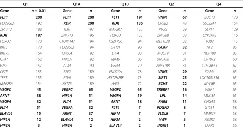
Using five disjoint test statistics increases the power over using a single statistic. Further test statistics did not further increase power (results not shown). Table 3 shows that there is a tendency for false positives to be found at the same genes over all replicate simulations, even for the
derived traits. This table also informs us that although phenotype Q4 is well behaved for data set 1, across all data sets there is a tendency for false-positive results to be seen in the same genes. Using the residual derived pheno-type Q4A corrected this problem (results not shown).
Table 2 Summary results for data set 1
Q1 Q2
Gene Q1 rank Q1A rank Q1B rank p-value for Q1 p-value for Q1A p-value for Q1B Gene Q2 rank p-value for Q2
FLT1* 1 1 1 0.0000 0.0000 0.0000 LRRC18 1 0.000441
ZNF91 2 5 6 0.0000 0.0000 0.0002 WDFY4 2 0.000441
FLJ22662 3 22 900 0.0000 0.0000 0.2604 SPAG8 3 0.000453
ZNF454 4 3 27 0.0000 0.0000 0.0044 RARB* 24 0.004243
KRT3 5 12 134 0.0000 0.0000 0.0285 GCKR* 28 0.005489
MAP2K6 6 16 834 0.0000 0.0000 0.2360 VNN1* 42 0.00835
ZNF568 7 4 118 0.0000 0.0000 0.0244 BCHE* 358 0.063238
BRCA1 8 15 58 0.0000 0.0000 0.0115 SIRT1* 382 0.068709
RGPD8 9 7 140 0.0000 0.0000 0.0301 INSIG1* 391 0.07131
KDR* 14 2 15 0.0001 0.0000 0.0018 VNN3* 639 0.128922
VEGFC* 15 238 26 0.0001 0.0090 0.0044 LPL* 1,443 0.382003
VEGFA* 157 197 282 0.0086 0.0062 0.0717 PLAT* 1,833 0.514235
ELAVL4 312 729 1,248 0.0281 0.0983 0.3655 VWF* 2,071 0.59704
ARNT* 653 1,086 983 0.1025 0.2037 0.2872 PDGFD* 2,426 0.716842
FLT4* 1,352 788 1,757 0.3187 0.1173 0.5233 VLDLR* 2,691 0.811708
HIF1A* 1,563 998 1,660 0.3930 0.1814 0.4937 SREBF1* 2,891 0.883901
Allp-values based on 106
randomizations. Ranks are the rank of the genes when ordered byp-value. Genes with asterisks indicate true associations with trait. Genes were chosen on the basis of rank for Q1 analyses or of being true.
●
Observed
−
log
10 Q1B Q2 Q4
0.0 0.5 1.0 1.5 2.0 2.5 3.0 3.5
0123456
False Positive Rate
Tr
ue P
ositiv
e Rate Q1B Q2 Best node
Best 5 disjoint nodes
Figure 4Power calculations. The left-hand plot gives a quantile-quantile plot forp-values from the analysis of data set 1. The solid line is the expected result. In the right-hand panel true-positive proportions are plotted against false-positives for varying significance level. This
Discussion and conclusions
The methods in QTLTree described here are a quick way to collapse the information contained in genotypes within a gene into a form that allows quick calculation of an optimum set of SNPs or combination of SNPs. Within the R environment, the method can also be used to interactively explore the sets of SNPs that may be affecting a quantitative trait. The methods seem to be able to detect an appreciable proportion of genes under-lying variation in phenotypes, although the large number of detected loci that do not contribute to variation using the raw trait data is worrying, because within-population randomization should account for any simple differences between populations. Because different levels of struc-ture exist within the data and because gene-environ-ment-region interactions are possible (e.g., the age structure differs between populations, and the values of the Q1 and Q4 phenotypes depend on age), we attempted a further level of correction. Using derived phenotypes after regressing on correlated phenotypes and PC loadings improved the type I error rates while not reducing the power for realistic false-positive rates.
Plots of PC loadings produced some unusual results that looked different from those from SNP arrays [8]. These are also seen in the correlations of Table 4, where PC loadings 1, 2, and 4 are significantly corre-lated with phenotypes Q1 and Q4. Because, from the answers to the GAW17 simulation, the sequenced genes
have no direct effect on phenotype Q4, the association of Q4 with PC loading 2 is most likely through both being associated with age. The correlation disappears when we take the residual after correcting for age, sex, and smoking status. Associations with the first loading, which explains more than 30% of the variation in the sample, are more difficult to explain because the first loading is correlated with the average heterozygosity (Figure 1; Table 4). Although this may reflect an under-lying variation in heterozygosity between people, it seems more likely that it reflects differences in coverage
Table 3 Summaries of repeatable significant results over 200 data sets
Q1 Q1A Q1B Q2 Q4
Gene n≤0.01 Gene n Gene n Gene n Gene n
FLT1 200 FLT1 200 FLT1 191 VNN1 67 BUD13 170
FLJ22662 192 KDR 200 KDR 135 OR5B2 48 SLC22A1 154
ZNF713 188 TERT 197 MAP2K7 135 PTGIS 39 SEPT1 129
KDR 187 ZNF713 196 FOXO3 133 ZNF568 38 CYP3A43 116
FOXO3 170 C1ORF147 194 HSZFP36 94 METTL2B 32 TOB2 115
KRT3 170 FLJ22662 194 EPHB1 90 GCKR 32 NF2 85
KRT75 164 OR6C4 192 LRP4 88 MUC19 31 NUP188 83
GRK1 162 PRKCH 192 RBM6 86 UNC45B 31 OR10T2 68
E2F2 157 ALX4 190 GRIA4 79 ZNF518B 31 C16ORF55 67
CETP 155 E2F2 189 FNDC3A 78 VNN3 29 ICAM4 65
TERT 155 ETV6 189 HIST2H2BE 73 SIRT1 25 LOC1001316 65
MAP2K6 154 KRT75 189 HAS3 72 BCHE 22 MYCBP 65
VEGFC 45 VEGFC 65 VEGFC 65 SREBF1 16 WBP1 65
ARNT 38 HIF1A 51 VEGFA 19 LPL 14 MUC3A 61
VEGFA 32 FLT4 51 ARNT 18 RARB 11 CNGA3 58
FLT4 51 VEGFA 32 FLT4 7 PDGFD 8 GTSE1 58
ELAVL4 15 ARNT 37 HIF1A 7 VLDLR 7 MMP27 58
HIF1A 12 ELAVL4 12 HIF3A 2 VWF 3 PIK3R2 58
HIF3A 3 HIF3A 2 ELAVL4 2 INSIG1 1 TAAR5 56
All significant results are based on a noncorrected significance level of 0.01. Numbers are the number of replicates where a gene was found to be significant (out of 200). Columns show the top results and those from true genes (bold). The maximum number of significant tests for Q4A was 8. All significance tests are based on 105
permutations.
Table 4 Correlations between population statistics and phenotypic traits
Trait Average heterozygosity
Rotation 1
Rotation 2
Rotation 3
Rotation 4
Age 0.02 0.14 0.16 0.07 0.06
Smoke −0.01 −0.04 −0.05 0.04 0.01
Q1 0.16 −0.15 −0.07 0.05 −0.19
Q2 0.05 −0.01 0.01 −0.04 −0.05
Q4 −0.06 −0.09 −0.12 −0.07 −0.03
Q1A 0.17 −0.21 −0.12 0.02 −0.24
Q1B 0.02 0.00 −0.01 −0.01 0.00
Q4A −0.10 0.06 0.02 −0.02 0.06
Affected 0.14 0.02 0.09 0.07 −0.05
in sequencing samples, because samples with higher coverage tend to have more variants called.
The strong false-positive signals with the raw data lead us to ask, can the difference in the number of variable sites between individuals explain the inflated errors in Q1? To test this for phenotypes Q1 and Q2, we created data sets with just the SNPs that affected disease and all non-disease-causing SNPs. The correlation across indivi-duals between average heterozygosity for SNPs affecting Q1 and average heterozygosity for SNPs not affecting Q1 is 0.22 (Pearsonr2,p= 5.6 × 10⁻⁹), and the correla-tion for Q2 isr2= 0.14 (p= 2 × 10⁻⁴). This may explain some of the false positives. Although such problems are unlikely to arise for real data, they emphasize the diffi-culties that may crop up in future studies using next-generation sequencing technologies if case and control subjects are not treated in the same way and if genotyp-ing and variant callgenotyp-ing are not performed blind to dis-ease status.
Acknowledgments
We thank Rita Cantor, the participants in GAW17 Group 13, and two anonymous reviewers for helpful discussions on the paper. Financial support was provided to DTH by the British Heart Foundation and to IJW and RAJH through Wellcome Trust grant 087436. The Genetic Analysis Workshops are supported by National Institutes of Health grant R01 GM031575.
This article has been published as part ofBMC ProceedingsVolume 5 Supplement 9, 2011: Genetic Analysis Workshop 17. The full contents of the supplement are available online at http://www.biomedcentral.com/1753-6561/5?issue=S9.
Authors’contributions
IJW wrote the computer code, carried out statistical analyses and drafted the manuscript. RAJH and DTH assisted with statistical analyses and helped to draft the manuscript. MSK conceived the statistical methodology. All authors read and approved the final manuscript.
Competing interests
The authors declare that there are no competing interests.
Published: 29 November 2011
References
1. Neale BM, Sham PC:The future of association studies: gene-based analysis and replication.Am J Hum Genet2004,75:353-362.
2. Madsen BE, Browning SR:A groupwise association test for rare mutations using a weighted sum statistic.PLoS Genet2009,5:e1000384.
3. Dering C, Pugh E, Ziegler A:Statistical analysis of rare sequence variants: an overview of collapsing methods.Genet Epidemiol2011,X(suppl X):X-X. 4. Cui Y, Kang G, Sun K, Qian M, Romero R, Fu W:Gene-centric genomewide
association study via entropy.Genetics2008,179:637-650. 5. Liu JZ, McRae AF, Nyholt DR, Medland SE, Wray NR, Brown KM, AMFS
Investigators, Hayward NK, Montgomery GW, Visscher PM,et al:A versatile gene-based test for genome-wide association studies.Am J Hum Genet
2010,87:139-145.
6. Sevon P, Toivonen H, Ollikainen V:TreeDT: tree pattern mining for gene mapping.IEEE/ACM Trans Comput Biol Bioinform2006,3:174-185. 7. Christensen GB, Lambert CG:Search for compound heterozygous effects
in exome sequence of unrelated subjects.BMC Proc2011,5(suppl 9):S95. 8. R Development Core Team:R: a language and environment for statistical
computing.Vienna, Austria, R Development Core Team; 2010. 9. Almasy LA, Dyer TD, Peralta JM, Kent JW Jr., Charlesworth JC, Curran JE,
Blangero J:Genetic Analysis Workshop 17 mini-exome simulation.BMC Proc2011,5(suppl 9):S2.
10. Li JZ, Absher DM, Tang H, Southwick AM, Casto AM, Ramachandran S, Cann HM, Barsh GS, Feldman M, Cavalli-Sforza LL,et al:Worldwide human relationships inferred from genome-wide patterns of variation.Science
2008,319:1100-1104.
11. Schwarz G:Estimating the dimension of a model.Ann Stat1978, 6:461-464.
doi:10.1186/1753-6561-5-S9-S98
Cite this article as:Wilsonet al.:Finding genes that influence quantitative traits with tree-based clustering.BMC Proceedings20115 (Suppl 9):S98.
Submit your next manuscript to BioMed Central and take full advantage of:
• Convenient online submission
• Thorough peer review
• No space constraints or color figure charges
• Immediate publication on acceptance
• Inclusion in PubMed, CAS, Scopus and Google Scholar
• Research which is freely available for redistribution