Laboratory modelling of the wind-wave interaction with modified
PIV-method
Daniil Sergeev1,2*, Alexander Kandaurov1,2, Yuliya Troitskaya1,2, Guillemette Caulliez3, Maximilian Bopp4, Bernd Jaehne4
1Institute of applied physics RAS, Geophysical Research Division, 603950 Ulyanova st. 46, Nizhny Novgorod, Russia 2
Lobachevsky state university of Nizhny Novgorod, 603950 Prospect Gagarina 23, Nizhny Novgorod, Russia 3
Mediterranean Institute of Oceanography, Avenue de Luminy 163, 13009, Marseille, France 4
Insititut fur Umweltphysik Im Neuenheimer Feld 229 69120, Heidelbeg, Germany
Abstract. Laboratory experiments on studying the structure of the turbulent air boundary layer over waves were carried out at the Wind-Wave Flume of the Large Thermostratified Tank of the Institute of Applied Physics, Russian Academy of Sciences (IAP RAS), in conditions modeling the near water boundary layer of the atmosphere under strong and hurricane winds and the equivalent wind velocities from 10 to 48 m/s at the standard height of 10 m. A modified technique of Particle Image Velocimetry (PIV) was used to obtain turbulent pulsation averaged velocity fields of the air flow over the water surface curved by a wave and average profiles of the wind velocity. The main modifications are: 1) the use of high-speed video recording (1000-10000 frames/sec) with continuous laser illumination helps to obtain ensemble of the velocity fields in all phases of the wavy surface for subsequent statistical processing; 2) the development and application of special algorithms for obtaining form of the curvilinear wavy surface of the images for the conditions of parasitic images of the particles and the droplets in the air side close to the surface; 3) adaptive cross-correlation image processing to finding the velocity fields on a curved grid, caused by wave boarder; 4) using Hilbert transform to detect the phase of the wave in which the measured velocity field for subsequent appropriate binning within procedure obtaining the average characteristics.
1 Introduction
The interaction between wind flow and surface waves is one of central problems of the study and parameterization of exchange processes in boundary layers of the atmosphere and ocean [1]. Of special interest is the case of steep and breaking waves forming at a strong wind. But carrying out field measurements of air flows, wave parameters for such conditions is very difficult problem (see. [2]). That is why laboratory modeling is used [3–5] to simulate conditions up to severe weather. The main difficulties in the experimental study of a turbulent air flow over a wavy water surface in laboratory conditions are connected with measuring wind characteristics near the water surface, especially in wave troughs, where one can expect the appearance of the most interesting features of this flow, such as shielding and separation of the flow. The technique Particle Image Velocimetry PIV is best fit for measuring the air flow in wave troughs and water flows close to the surface. In [6–8], the experience of using the PIV technique for measuring the air flow velocity over a wavy surface was presented. In [8], the structure of average velocity fields in the air flow and their perturbations initiated by waves, as well as the structure of turbulent stresses, were successfully studied.
However, those measurements were carried out at low wind velocities.
The subject of this work is studying the characteristics of air flows, waves, under conditions of breaking of waves with the formation of sprays near a wavy surface, in particular, in wave troughs due to high wind speeds.
Earlier, measurements under conditions of strong winds with an equivalent wind velocity U10 > 25 m/s in
the laboratory modeling of extreme meteorological conditions were carried out only using contact gages (Pitot tubes and hotwires/hotfilms) at a consider able distance from surface wave crests [3–5, 9]. The measurement region was positioned above the layer of constant fluxes, where the velocity profile is logarithmic and its parameters (the friction velocity and roughness height z0) could be determined directly using the profile
method. Therefore, and z0 have to be determined using
the self-similarity property of the velocity profile of the flow in channels, as it was done in [4]. However, to refine the self-similar form of the velocity profile, it is necessary to measure the flow velocity as close to the water surface as possible [10].
wide range of the winds (up to strong and hurricane conditions) with use of a specially modified PIV technique.
2 Experimental setup and measuring
technique
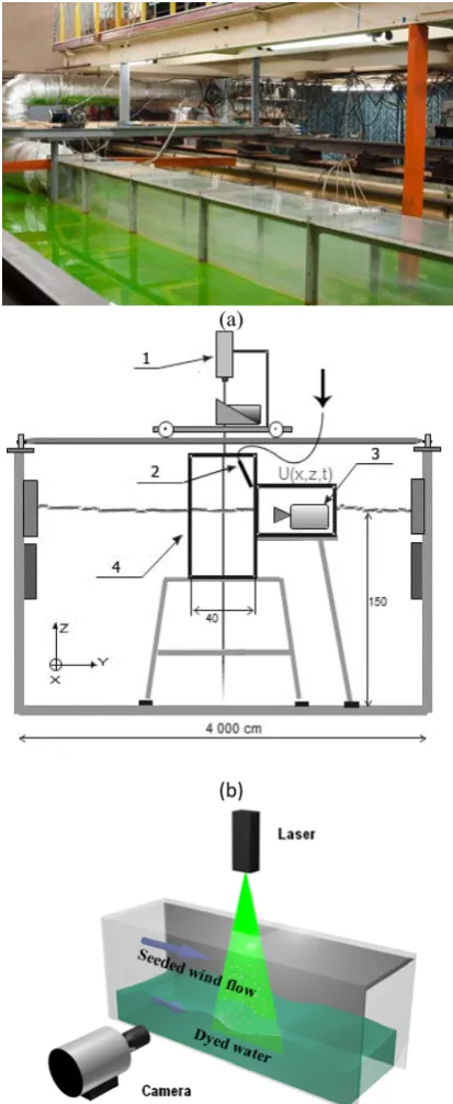
Experiments were carried out on the Wind-Wave Flume of the Large Thermostratified Tank of IAP RAS (overview on Fig. 1 a). The length of the air flow channel with a cross section of 0.4 × 0.4 m is 10 m over the water surface. A detailed description of this setup and principles of design and control for the air flow in it were presented in [4, 5]. The general scheme of the experiments is presented in Fig. 1 b. In addition to PIV methods, which were the main tool in the presented investigations, earlier approbated contact ways of measurements were used. In the working section of the channel, at a distance of 7 m from the entrance, average profiles of the air flow velocity were measured using a Pitot tube. The air flow in the channel was visualized using polyamide particles with an average diameter of 10 m and density of 1.02 g/m3. The inertial time was 2 × 10⁻⁴ s. The seeding device was similar to that used in [8] and positioned at the entrance of the channel at a distance of 6 m from the detection area. The test experiments demonstrated that the system brings no distortions to the wind flow in the region of measurements. To apply the PIV method (principal scheme shown on the Fig. 1 c), the motion of particles in the air in the region of measurements was illuminated by a laser sheet along the channel axis 8 m from the inlet. The laser sheet is formed by a cylindrical lens from a vertical laser beam (a continuous Nd YAG laser, 532 nm, 4 W). The width of the illuminated area was varied choosing the radius of the cylindrical lenses and their mutual arrangement. The motion of particles introduced into the air flow and water surface which were illuminated by the laser sheet was taken from the side by VideoSprint high speed camera positioned horizontally in a sealed box (see Fig. 1b). The camera was positioned horizontally and the level of its optic axis was above the level of the water surface by 8 cm. The focal plane was at a distance of 77 cm from the laser knife. The size of the taken area was from (66.4 – 16 mm) × 256 mm (the horizontal size of a frame decrease with an increase in filming speed). A droplet removal system in the form of a metal tube blown with supplied compressed air was mounted from the internal side of the channel side wall through which the filming was performed. According to test experiments, the system introduced no distortions to the wind flow in the region of measurements.
The experiments were carried out at four values of air flow rates in the channel: 1.1, 1.6, 2.2, and 2.7 m3/s; as it is shown below, this corresponds to equivalent wind velocities at heights of 10 m, U10, 11, 20, 37, and 48 m/s,
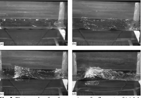
respectively. In two last cases, a strong breaking of waves with the formation of white caps and intense generation of sprays was observed (see photographs in Fig. 2). For each wind velocity, 30 implementations were taken, 3000–4500 frames in each implementation.
The filming speed was 1500, 3000, 5000, and 6000 fps; the exposure time was from 50 to 14 s.
()
(b)
Fig. 1. a) Wind-Wave Flume of the Large Thermostratified Tank of IAP RAS (air channel in the center) b) principal scheme of experimental setup in the working cross-section of the wind channel 1- laser, 2 – droplets blow-off system, 3 – high-speed camera, 4 – wind-wave channel. c) scheme of PIV-method using.
3 Experimental data processing
images from a highspeed camera, a stepwise algorithm [11] was developed based on the Canny method [12]. That method operated well under conditions of weakly breaking waves. However, with an increase in the air flow velocity, a transition to a rather intense breaking with the formation of sprays and whitecaps was observed. In this order, a combined method of measuring the elevation of the water surface was used. In this method, optical measurements were completed by contact measurements using a wire wave recorder mounted on the channel axis near the edge of the laser sheet. The records of the level elevation and high speed camera were synchronized. The final form is a combination of data obtained by contact and noncontact ways; with an increase in wind velocity, the role of contact measurements increased up to a full substitution of optical measurements for the case of flow rate of 2.7 m3/s (see Fig. 3).
Fig. 2. Photographs of surface waviness for flow rate of (a) 1.1, (b) 1.6, (c) 2.2, and (d) 2.7 m3/s.
After finding the surface shape, velocity fields were calculated by the cross-correlation method over a curvilinear grid taking into account the current shape of the surface [8]. We used a modified PIV processing method based on adaptive finding for the shift of the cross-correlation function (from now on, briefly CCF) peak for rectangular elements of the image for two sequential frames. The space on the grid of the velocity field calculation was 3.2 mm. To increase the algorithm accuracy due to a decrease in the search window size, the processing was performed in two stages. At the first stage, using a window with dimensions of 128 × 64 px, the profile of the average horizontal shift of particles for each wind velocity was found.
At the second stage, the comparison window was shifted to the magnitude of the shift found at the first stage. The size of the search window could be less than the final shift of particles, which increased the spatial resolution of the method, accelerated the processing, and made it possible to obtain more data. The CCF maximum was searched by the adaptive method during two iterations by analogy with [8]. At the first passage, the shift over the window with a larger size (32 × 32 px or 6.4 × 6.4 mm) was approximately determined; then, an after search was performed with allowance for the calculated shift for a window with a lesser size (8 × 8 px or 1.6 × 1.6 mm). To increase the accuracy at the last
step of cross correlation, an algorithm of subpixel approximation of the peak by a Gaussian two-dimensional profile (see [8]) was applied; this allows one to take into account CCF values at points near the maximum.
Fig. 3. Example of finding the surface shape (a) by the laser optical method and by data from a wave recorder in the case of (b) a foam line and (c) the rear front of the wave.
Data that do not satisfy the quality criteria were eliminated from further processing. In particular, windows with an insufficient quantity of particles were eliminated from the processing. For each image, points corresponding to high values of the brightness gradient were found using the Sobel operator. These points correspond to edges of particle images in the frames. For each window, the number of similar boundary pixels was calculated. The threshold value of the brightness gradient in the process of searching the edges was matched so that no boundary pixels fell in regions without particles. The cross correlation was performed only with windows in which at least one boundary pixel was present. In this process, if the number of boundary pixels considerably exceeded the average number, flares, spindrifts, or a foam line were most often present in part of the image corresponding to this region; as a consequence, the shift calculated for it was not taken into account in the process of further averaging. Regions for which the value of the CCF maximum considerably differs from the typical value in the implementation were also not taken into account, because such regions most often corresponded to the case of a particle escaping from the laser sheet during the interval between frames.
At strong winds, the inhomogeneity of seeding increased, which resulted in considerable discontinuities (the absence of data) in time dependences of velocities at fixed horizontal coordinates. Despite measures for the removal of droplets, optical distortions increased with an increase in the wind velocity. This resulted in decreasing of accuracy.
water surface elevations presented in several equidistant vertical cross sections for each frame. There were from three to seven such cross sections in a frame (depending on the flow rate).The position of the surface for each vertical column of the velocity field was calculated using linear interpolation. Thus, each column has its own dependence of the surface position on time.
Wave number spectra of waving have a pronounced peak, and deviation of the water surface from the horizontal is determined mainly by the fundamental wave harmonic. For this reason, averaging over the phase of the fundamental wave harmonic was performed. Frequency filtering of time realizations obtained in the aforementioned way was performed over a band with a width of 2 Hz near the peak frequency determined for each wind velocity by time realizations from the wave recorder. Such filtered realizations with a removed constant component fit well for determining the wave phase by use of the Hilbert transform. Using the economical algorithm of the fast Fourier transform, the Hilbert transform permits one to determine the amplitude and phase of surface elevation as a function of time.
To obtain velocity fields averaged over turbulent fluctuations, conventional averaging at a fixed phase was performed. To reduce errors connected with the insufficient number of measurements, the data were binned in phase intervals of 18°, which yields 20 different binns of the phase.
The averaging was performed in two ways:
(i) Averaging over fixed horizons (Fig. 4a). The velocity fields were divided into horizons with a step of 32 px (6.4 mm of the real height). For each horizon and each phase, velocities were accumulated from the whole realization and then averaged.
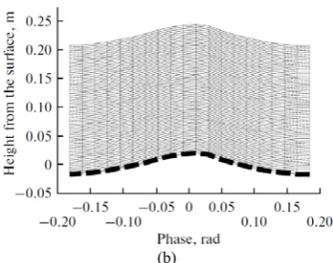
(ii) Averaging over a fixed distance from the surface (Fig. 4b). For each frame in each column of the grid, a cell with the same number was chosen; in the curvilinear coordinate system used, this meant a fixed distance of the point from the surface. The data from corresponding similar cells over the height and phase were accumulated from the whole realization and then averaged.
(a)
(b)
Fig. 4. Examples of a grid over which the velocity was averaged: (a) averaging over fixed horizons and (b) averaging over the distance from the surface.
4 Results
Pictures of turbulentpulsation averaged velocityfields of the air flow were obtained for both ways ofaveraging. In curvilinear coordinates, by analogy with [8], the vertical coordinate is counted from the position of the water surface at each instant of time. Theposition of the average surface level was taken as zeroin rectangular coordinates. The horizontal coordinateis the wave phase for a given point ij recalculated usingthe value of the wavelength Ȝ determined by the dispersion relation for waves on deep water for a frequency corresponding to the peak in the center of thespectrum for each value of the wind velocity:
2 x M O
S
Examples of flow fields for both averaging are presented in Fig. 5.
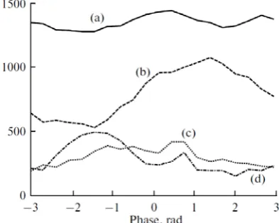
The number of points satisfying the criteria of data quality is different for the same distance from the surface in different phases. This difference is especiallyseen near the surface, where the decrease in the quantity of data satisfying the quality criterion from the leeward side of the wave crest (negative values of thephase in Fig. 6) caused by decrease in the number oftracing particles in this region at the instant of shooting due to the shielding of the wind flow by the wavecrest. Note that, for the cases of two high wind velocities (U10 of 37 and 48 m/s),
an inverse picture isobserved: the number of points satisfying the criteria ofdata quality becomes larger from the leeward side ofthe crest. This can be connected with the appearance of sprays, which are intensely generated at velocities U10 > 25 m/s. The droplets
() 1.1 m3/s
(b) 1.6 m3/s
(c) 2.2 m3/s
(d) 2.6 m3/s
Fig. 5 (a) –(d)Velocity fields averaged over ensemble, for fixed phase along the horizons in Cartesian coord. Color indicates number of points in ensemble of averaging for each cell.
(e) 1.1 m3/s
(f) 1.6 m3/s
(g) 2.2 m3/s
(h) 2.6 m3/s
Since the droplet velocity is lower than the wind velocity, this leads to an erroneous underestimation of the air flow velocity near the surface. The different number of particles in different phases makes it necessary to apply conventional averaging over the phase toobtain correct results.
Fig. 6. Number of cells taken into account in the averaging as a function of the wave phase for different values of air flow rate: (a) 1.1, (b) 1.6, (c) 2.2, and (d) 2.7 m3/s. The function is averaged over height inside the nearwater layer with a thickness of 5 cm.
Velocity values obtained using thePitot tube always turned to be lower than those obtained in PIV measurements.Note that the PIV technique is a direct method ofdetermining the air flow velocity; in contrast to it, thePitot tube is an indirect method of estimating the flowvelocity by pressure and the underestimation of theflow velocity by the Pitot tube probably indicates the presence of a systematic error.
Fig. 7. Profiles of the average horizontal component of wind velocity in the channel for different values of air flow rate: (a) 1.1, (b) 1.6, (c) 2.2 m3/s. The profiles were obtained by averaging PIV data over curvilinear coordinates (dashed lines), Cartesian coordinates (solid lines), and based on data from the Pitot tube (symbols). The dotted vertical lines shows average levels of wave crests for each case. For the flow rate 2.7 m3/s.
Fig 7 shows also the air flow velocity profiles obtained by averaging measurement data using the PIV method. Two ways of averaging the velocity field were used: over horizons (the solid line) and curvilinear coordinates (the dashed line).
Both the velocity profiles have a similar shape and close values; they agree with each other well in the region above wave crests. The main difference between them is that averaging over curvilinear coordinates can yield air flow velocities in wave troughs, while averaging over horizons can yield the vertical profile of the average wind velocity only above wave crests. In connection with this, the aerodynamic drag factor of the water surface was determined by dependences obtained by averaging over curvilinear coordinates.
5. Conclusion
Laboratory experiments on studying the structureof the turbulent air boundary layer over waves werecarried out at the WindWave Channel, IAP RAS,under conditions
ٝ
modeling the near water boundary layer of the atmosphere under strong and hurricanewinds. Air flow in the channel with a square cross section of 0.16 m2 was created by fan. The air flow ratetook values of 1.1, 1.6, 2.2, and 2.7 m3/s, which corresponded to estimate values of equivalent wind velocities from 10 to 48 m/s at the standard height of 10 m.
A modified technique of Particle Image Velocimetry (PIV) was used to obtain turbulent pulsation averaged velocity fields of the air flow over the water surface curved by a wave. We emphasize that such remote methods permit one to obtain the air flow velocity field also below wave crests in wave troughs. Using wave phase averaging at fixed distances from the water surface, average profiles of the air flow velocity were obtained in curvilinear coordinates following thewave. Note that measurements couldbe reliably performed only using the PIV technique. Using contact measurements (Pitot tube), profiles of the air flow velocity over wave crests were measured in Cartesian coordinates. To compare measurement results obtained by two techniques, measurement data obtained by the PIV technique were also expressed in Cartesian coordinates. Both experimental methods yielded close results at distances of more than 10 mm from wave crests. But introducing the Pitot tube with a diameter of about 10 mm into the flow could resulted in considerable distortions of the flow close to the water surface. Parameters of the air flow (friction velocity and drag coefficient of the surface) could be further determined by extrapolating the logarithmic part of the velocity profile, and their dependencies on the wind speed could be obtained.
scientific and technological complex for 2014-2020" (grant agreement 14.616.21.0059, a unique identifier RFMEFI61615X0059 project)
References
1. C.W. Fairall, E.F. Bradley, J.E. Hare, A.A. Grachev, J.B. Edson, Climate., 16(4). 571 (2003) 2. M.D. Powell, P.J. Vickery, T.A., Nature. 422.,
279(2003).
3. M.A. Donelan, B.K. Haus, N. Reul, W.J. Plant, M. Stiassnie, H.C. Graber, O.B. Brown, E. S. Saltzman, Geophys. Res. Lett., 31, L18306 (2004) 4. Yu. I. Troitskaya, D.A. Sergeev, A.A. Kandaurov,
G.A Baidakov, M.A. Vdovin, V.I. Kazakov JOURNAL OF GEOPHYSICAL RESEARCH,
117(C00J21), 13(2012)
5. Yu. Troitskaya, D. Sergeev, A. Kandaurov and V. Kazakov., (Recent Hurricane Research - Climate, Dynamics, and Societal Impacts, InTech, 2011) 6. Reul, N., H. Branger, and J.-P. Giovanangeli,
Bound.-Layer Meteor., 126, 477 (2008)
7. Veron, F., G. Saxena, and S. K. Misra, Geophys. Res. Lett., 34, L19603(2007).
8. Yu. Troitskaya, D. Sergeev, O. Ermakova, G. Balandina, J. Phys. Oceanogr., 41, 1421(2011) 9. 9. C.T. Hsu, E.Y. Hsu, R.L. Street, J. Fluid 105,
87(1981)
10. Hinze J. O. (Turbulence: An Introduction to its Mechanism and Theory, McGraw-Hill. 1959) 11. D. Sergeev, A. Kandaurov Yu. Troitskaya, Proc.
Opt. Meth. Flows Invest. 90 (2011).