1
Relative abundance of insect predators varies among rice plots as a function of
2
surrounding landscape
3 4
Md. Panna Ali1*, Mir Md. Moniruzzaman Kabir1, Sheikh Shamiul Haque1, Abeer Hashem3,4 5
and Elsayed Fathi Abd_Allah5
6 7
1Entomology Division, Bangladesh Rice Research Institute, Gazipur-1701, Bangladesh. 8
2Genetic and Plant Breeding Division, Bangladesh Rice Research Institute, Gazipur-1701, 9
Bangladesh. 3Botany and Microbiology Department, College of Science, King Saud
10
University, P.O. Box. 2460 Riyadh 11451, Saudi Arabia. 4Mycology and Plant Disease
11
Survey Department, Plant Pathology Research Institute, Agriculture Research Center, Giza,
12
Egypt. 5Plant Production Department, College of Food and Agricultural Sciences, King Saud
13
University, P.O. Box. 2460 Riyadh 11451, Saudi Arabia.
14
*Corresponding author email address: [email protected]
15 16
Abstract
17
Relationships among the population abundance of four predator groups for rice insect pests,
18
namely: carabid beetles, staphylinid beetles, green mirid bugs, and spiders in three landscape
19
categories were evaluated. Both rice plots and the associated bund margins of these rice plots
20
found among three Bangladesh landscape categories were sampled by sweep net. The results
21
revealed that the abundance significantly varied across landscapes. The rice landscape of one
22
location harbored higher numbers of a specific predator than other location in other regions of
23
Bangladesh. The results also showed a dependency on the width of the rice bund margins of
24
the rice plots, where spiders populations increased with increased bund widths, but the
25
population abundance of these predators did not depend on the diversity of the number of
26
weed species found on the rice bund margins. The relative abundance of predator populations
27
also significantly differed among the three landscapes, with the green mirid bug having the
28
highest number among the four predators. This study indicates that predators of rice insect
29
pests are highly landscape specific. In order to design integrated pest management systems
30
for different Bangladeshi rice production locales, considerations unique to the characteristics
31
of each locale are necessary. Preliminary efforts to apply variography analyses to the RED
32
spectral band of LANDSAT 8 imagery from December 2016 are presented as first step
33
toward learning a suite of methods which describe useful local characteristics affecting rice
34
pest predators.
35
Keywords: Rice landscape, natural enemies, location, population dynamics, variography,
36
LANDSAT 8
37
38
Introduction
39
Rice (Oryza sativa L.), the staple diet of over half of the world's population, is grown
40
on over 158 million hectares worldwide, which produced over 465 million tons in 2012. In
41
Bangladesh, rice occupies about 77% of the cropped areas (Bhuiyan et al. 2004) which
42
account for a total 11.6 million hectares to produce 34 million tons of milled rice (IRRI,
43
2014). Bangladesh has 3 rice growing seasons (BRRI, 2016); namely, Aus (monsoon rice),
44
Aman (rain-fed with supplemental irrigation) that has two types of production (Broadcasted
45
Aman and Transplanted Aman), and the Boro (irrigated and well managed rice) season. Rice
46
is cultivated throughout the year and the intensity of cultivation increases day by day to meet
47
demands from more people living in Bangladesh every year. The rice agro-ecosystem covers
48
the major part of the non-urban land area in Bangladesh. These rice eco-systems are inhabited
49
by hundreds of arthropod species (Heong 2011) which perform various ecological functions,
50
such as herbivory (feeding on the rice plants), predation, parasitization, pollination,
51
decomposition, and nutrient cycling.
52
To date, 232 rice insect pests and 375 beneficial arthropod species have been
53
identified from the rice ecosystem in Bangladesh (Ali et al., 2017). However, while fewer
54
than 20 species are of significance in causing yield losses when they occur in sufficiently
55
large numbers in India, Bangladesh, numbers up to 20-33 total species considered of
56
importance to cause economic damage to rice production (BRRI, 2007). These pests, in turn,
57
are subjected to attack by predators and parasitoids, and thus, are often naturally kept in
check. This intricate food web of relationships among the rice plants, the pests, and the rich
59
biodiversity of natural enemies constantly strives to maintain an equilibrium preventing
60
abnormal increases in abundance of pest species. This equilibrium level of a rice ecosystem is
61
also often broken due to heavy use of synthetic fertilizers and pesticides. The breakdown in
62
‘ecological resilience’ of a rice farm induces pest’s outbreaks (IRRI, 2011) that causes
63
economic damage to rice growers worldwide, despite usage of insecticides.
64
Scientists have long claimed that indiscriminate use of pesticide is the main reason for
65
major outbreaks of insect pests in many kinds of crop production plots (Stern et al., 1959). A
66
recent example in rice is the increase in outbreak frequency of Nilaparvata lugens (brown
67
planthopper) over numerous Asian rice growing countries in recent years, 2005–2012
68
(Heong, 2010), due to adverse effects on planthopper natural enemies (NE) caused by
69
increased use of broad spectrum insecticides for control of other kinds of rice pests (Chien
70
and Cuong, 2009, Heong, 2009, Islam and Haque, 2009, Moni, 2011;2012, Luecha, 2010,
71
Matsumura and Sanada-Morimura, 2010, Soitong and Sriratanasak, 2012, Teo, 2011). The
72
use of pesticides increased in Bangladesh by 200% from 1997-2000, 250% by 2006 and by
73
nearly 500% by 2014 (BPCA, 2015). More than half of the amount of those insecticides was
74
applied against rice pests. Synthetic chemical-like insecticides are hazardous and harmful for
75
non-target organisms (e.g., Travisi et al., 2006, Ahmed et al., 2002; 2011). Besides just the
76
increasing usage of chemical insecticides over the years, other factors such as climate change
77
and landscape change also induce disappearance of NE from Bangladesh rice plots. Analysis
78
of
79
Natural enemies abundance in a crop plot vary with the apportionate areas of different
80
habitats that prevail in the surrounding landscape (Bianchi et al., 2006; Werling et al., 2011)
81
and possibly with differences in small scale changes in timing and choice of management
82
decisions (Willers et al. 2005; Shaw and Willers, 2006) for another insect pest, such as Lygus
lineolaris in Mid-South, USA, cotton. Landscape changes, which shape the habitat structure,
84
materials, and biotic interactions in agroecosystems, are also important factors driving pest
85
and NE population abundance (Woltz et al. 2012). Landscape characteristics can influence
86
pest and NE population in crop field. Recently, remote sensing method provide quickly
87
various types of surface monitoring data such as local, landscape, vegetation, specific crop,
88
water body and animal population. Variogram analysis of the data for spatial heterogeneity
89
can help identify explain related ecological phenomena (Zhaofei et al. 2013). Here we intend
90
to use variogram analysis and find their impact on landscape characteristic which also can
91
explain the pest and NE population abundance. It could also be used to improve quantitative
92
agricultural remote sensing monitoring in a spatial heterogeneity area as well.
93
Examining such kinds of impacts on pests or NE and understanding their mechanisms
94
may help to design pest management strategies at landscape scales (Wang et al. 2015).
95
However, the description of the abundance of NE in different Bangladesh rice landscape
96
categories remains elusive. Therefore, the objective of this study was to assess the abundance
97
of NE in different rice landscapes to help design pest management strategies influenced by
98
the different rice production seasons, types of production styles (i.e., small, household
99
farmers vs large, non-household farmers) and categories of landscape-scale agro-ecosystems.
100
In addition, variograms are used to analyze the landscape characterize based on LANDSAT 8
101
images collection. To target this objective we surveyed, recorded, and summarized the
102
abundance of several NE species from different rice landscapes in Southern Bangladesh.
103
Materials and Methods
104
The sampling experiments were conducted in three categories of landscape located in
105
Southern Bangladesh, or the Barisal Division, which includes within it the Barisal and
106
Jhalkathi Districts, where each district is further divided into two more smaller governmental
107
entities, known as the Upazila, and within these, the smallest one, known as a Union (Refer to
Fig. 1, where all but the Upazila are mapped). Each landscape category represents a unique
109
type within several Unions of these two Districts, and which are sufficiently describable to
110
permit replication (in geographic space at the Union designation) of each category. We
111
defined these rice landscapes within a buffer zone around each one, into three category
112
classes based on surrounding features and characteristics found within the buffer zone
113
surrounding candidate rice plots. Each landscape was replicated two times.
114
Landscape I ─ Rice plots in this category are typically surrounded by big and small
115
fruit trees, or forests (such as deciduous and coniferous trees). The entire rice plots, here, are
116
enclosed by densely perennial habitats, having fewer kinds of annual crops and lower
117
vegetational diversity. The perennial habitats are found in close proximity to rice plots, with
118
an range of distances from 10-30 m. The main feature of this landscape is the presence of
119
small, narrow (so called canal), drainage flows between the rice plots and (concrete) roads,
120
which always flows, and with some weeds growing in the canals. The canals are connected to
121
rice plots, which were very muddy types. The irrigation system of this landscape is comprised
122
of a shallow tube well. The width of rice bunds surrounding rice plot, are between 25-35 cm
123
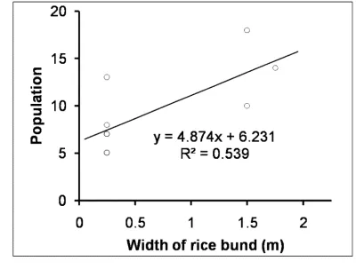
and separate one smallholder plot from another one. Landscape I replicates were selected
124
near Protap, in the Rajapur Upazila Union, and the Jhalokathi Sadar Union of southern
125
Bangladesh, and were of similar structure and composition by visual interpretations. The
126
specific location of this landscape is presented in Fig. 1A.
127
Landscape II ─ This category consists of rice plots, homestead trees, and a rain forest,
128
containing both small and big trees. The landscapes are located the Nalchity Upazila, in the
129
Jhalkati and Barisal Sadar Unions of southern Bangladesh, characterized by less muddy rice
130
plots found near roadsides, with a few fruit and forest trees found around the rice plots and
131
planted along the roadside. Any nearby perennial habitats were very far from the rice plots,
132
compared to Landscape I, with distances between 100-200 m. There are no canal or drainage
systems in this landscape and the irrigation system is comprised of deep tube wells. The
134
specific location of these landscape replicates is also shown in Fig. 1A.
135
Landscape III ─ This third category was selected near the Babuganj and Wazirpur
136
Upazilas, and only from the Barisal District of southern Bangladesh, and is found with an
137
irrigation system different from others. The specific locations of this landscape category
138
replicate is depicted too in Fig. 1. Here, a buried irrigation system was used and the rice plots
139
are surrounded by some local fruits and other cultivated trees, but slightly farther away from
140
the rice plots. Any areas of perennial habitats were very far from the rice plots, with distances
141
between 200-400 m. The roads were also 200-400 m farther away from the rice plots than
142
any roads if the other two landscape categories. Small, narrow trees were also found
143
alongside the roads. A narrow small canal was also present in this landscape, but that canal
144
was 300-400m away from the rice plots. Entire rice plots were divided into two separate, but
145
big parts, by a wide walking bund, with an additional irrigation channel located on this bund.
146
Rice plots from each landscape selected for study ranged 15-20 ha in area. The total
147
set of rice plots in each replicate was composed of 50-70 plots separated from each other by
148
bunds in each sample location among the landscape categories, except for Landscape III. In
149
the Landscapes I and II, each small plot was occupied by one smallholder rice farmer, whom
150
maintained their plots according to improved rice production technology. The size of farmers
151
plot ranged 1500-2500 m2. The plot size in Landscape III ranged between 1000 - 2000 m2,
152
and were farmed by smallholder farmers. The ‘plots’ for all replicates selected to record
153
arthropod populations was transplanted with BRRI dhan29 (a mega-rice variety in
154
Bangladesh). Four-6 plots from each landscape were considered for data collection.
155
For transplanting BRRI dhan29 in selected rice plots, farmers raised seedlings in a
156
seedbed. Seedbed management was performed according to the traditional farm practices
157
(BRRI, 2011). Before transplanting seedlings into candidate sample plots, land was well
prepared according to the common practice of wetland soil preparation followed by
159
laddering. Laddering is the cultural farming practices where the ladder is used to break down
160
clods and level the plot once or twice after ploughing. Thirty-five to 45 d old seedlings were
161
transplanted in selected rice plots during the Boro rice cultivation season in 2015-2016.
162
Standard transplanting space (20 x 20 cm2) was maintained. Fertilizers containing N, P, K, 163
and S were applied at the rates of 82, 15, 38, 10.6 and 2.7 kgha-1 respectively, using urea,
164
triple superphosphate (TSP), muriate of potash (MOP), and gypsum. The total amount of
165
TSP, MOP, gypsum, and 1/3 of the urea amount were applied during the final land
166
preparation period. The remaining urea was top dressed in two equal splits at 20 d after
167
transplanting (DAT) (or the early tillering stage) and 40 DAT (or the maximum tillering
168
stage), synchronized with irrigation or wet soil conditions, because the sampling experiment
169
was conducted under irrigation conditions. Pesticides were applied two times in all rice plots
170
across the tested landscapes. Therefore similar amount of pesticides were received by each
171
rice plot.
172
Arthropod populations were recorded from 4-6 plots of each replicated rice landscape
173
category which means 24-36 plots (4-6 plots x 6 landscapes). Two landscapes of each
174
category were considered for this study. The sampling was conducted two times. A sampled
175
plot was randomly selected from the entire set of rice plots found, as present in a replicated
176
landscape category. Arthropod populations were collected from both the chosen rice plot, and
177
its adjoining rice bund, using a sweep net. Durable insect sweep nets easily collected insects
178
from grass, fallow land, brush and the rice crops. Two times 20 complete sweeps were taken
179
to collect insect pests and their NE at maximum tillering stage of the rice crop at each sample
180
plot, because that stage of rice harbors a wider number of arthropods (Bari et al. 2016). The
181
collected insect pests and NE were sorted, identified, counted and written onto a data
182
collection sheet for every sampled plot. Each bund was covered by numerous weed species.
183
The number of weed species grown in the rice bunds was also recorded, but individual weed
species were not identified taxonomically, but instead to only estimate the total number of
185
weed diversity, as found on that bund. The width of each rice bund was also recorded using a
186
measuring scale. The plot used to collect arthropods using sweep net was also examined by
187
rice hills (for a total of 100 hills/sampled rice plot), to make additional observations on
188
infestations by insect pests that stay in the lower part of the plant. The sampled insect pests
189
observed in the tested plots in each landscape were negligible and avoid to present in the
190
paper. Therefore only NE populations were described here.
191
Relative abundance of NE populations was calculated using the following equation
192
(Rahman et al. 2014):
193
Relative abundance (%) = Total No. of individuals of each species
Total No. of of individuals of all species X 100
194 195
Data were analyzed by means of analyses of variance (one-way ANOVA), using landscape
196
category as the explanatory variable. Means were compared by Tukey’s test among the
197
landscapes (P < 0.05). The paired t-test was also performed to analyze the effect between rice
198
plot and bund. Data were transferred to logarithm scale in order to homogenize the variance.
199
Pearson’s correlation analysis was used to determine the correlation coefficients between NE
200
populations with rice bund’s width and number of weed species growing on the bund. All
201
statistical analyses were done using SPSS software, Version 16.0.
202
A LANDSAT 8, true color satellite image in TIFF format, (labelled,
203
LC08_L1TP_137044_20161130_20170317_01_T1) for late November, 2016, was obtained
204
from the United States Geological Survey (USGS) website for variography analyses. It was
205
hypothesized that variograms at the Union area extent of the 6 sampled landscapes and 12
206
more non-sampled, non-classed Unions for comparison, could be useful to aid in landscape
207
classifications of the other Unions of the Barisal and Jhalkarti Districts of the Barisal
208
Division of southern Bangladesh. The software package ERDAS IMAGINE® 2016 and ESRI
ARCGIS® 10.2, and SAS® software for PROC VARIOGRAM were utilized to process and
210
analyze the RED spectral pixels contained within the polygon feature layer of the selected
211
Unions (Fig. 1). This date was selected for its cloud free characteristics and because it was
212
not closely associated with the sampling times of the plot survey data, in order to examine
213
how non-seasonal information from satellite platforms may aid the ground survey results and
214
characterization of the sampled landscape classes.
215
Results
216
We have assessed four (4) different insect predators under the present study namely, spiders
217
─ a general predators group, the green mirid bug (GMB, Cyrtorhinus lividipennis Reuter) ─
218
an egg predator of planthoppers and leafhoppers of rice, the carabid beetles (CB) ─ predators
219
of several kinds of planthoppers and leaffolder larvae of rice, and the staphylinid beetles
220
(staphilinids) ─ a generalist predators of the nymphs of planthoppers. The number of insect
221
pest species found was negligible during this phenological stage while sampling NE, having
222
no effect on rice yields. The sampled plots (and plots) were also tracked up to harvesting
223
stage in order to detect if a significant number of pests occurred after data recording. The
224
investigated plots did not show any visual plot damage due to insect pests. But the number of
225
NE population varied among the landscapes and their population dynamic was described
226
below.
227
Spider: Spiders were significantly different among the landscape categories recorded from
228
the landscape I, landscape II and landscape III rice plots. The landscape I showed the highest
229
population numbers than that of the other two categories (Fig. 2). Number were significantly
230
higher in the rice (plot) plots than the rice bund in landscape I and landscape II, but the
231
highest population was found in rice bunds in the landscape III (Fg. 2; p = 0.001). The spider
232
populations also depended on the width of rice bund and a trend of increase followed the
233
increase with bund width (Fig. 3). A significant correlation existed between spiders and bund
width (Pearson’s correlation, r = 0.576; p = 0.050), but there was no correlation between
235
spider numbers and the number of weed species found in the bunds (Pearson’s correlation, r
236
= -0.119; p = 0.80). The relative abundance of spider population also significantly differed
237
among the different landscapes (Fig. 7).
238
Green mirid bug (GMB): Population of GMB was significantly different among the
239
landscapes. Rice plots located in landscape I showed the highest populations compared to that
240
of the other two (Fig. 4, df = 9, F = 167.58, p < 0.001), while the lowest population was
241
observed in the rice plots of landscape III. Similar number of GMB population was found in
242
the rice bund of both landscape I and landscape III and significantly less individuals were
243
observed on the rice bunds of landscape II (Fig. 4, df = 9, p <0.05). Populations of GMB
244
differed significantly between rice plots and rice bund among all landscapes (df = 9, p <
245
0.001). The relative abundance of GMB population also significantly differed among the
246
different landscapes (Fig. 7).
247
Carabid beetles (CBB): Populations of CBB significantly varied among all landscapes,
248
where landscape III showed the highest numbers in the rice plots than that of the other two
249
landscapes (Fig. 5, df = 9, F = 167.58, p < 0.001), with the least found in landscape II. In
250
regards to the rice bund, highest number of CBB population was found in landscape III and
251
the lowest population was observed in landscape I. The CBB population significantly varied
252
between rice plots and rice bund at every landscape (df = 9, p < 0.001). Like the spiders, the
253
CBB abundance also depended on the width of rice bund and increased with increased bund
254
widths. Significant correlation existed between these two variables (Pearson’s correlation, r =
255
0.423; p = 0.050). No significant correlation existed between CBB numbers and number of
256
weed species found on the bund (Pearson’s correlation, r = 0.119; p = 0.78). The relative
257
abundance of CBB also significantly differed among the different landscapes (Fig. 7).
Staphylinid beetle: Landscape III contained significantly more staphylinids than landscapes
259
I and II. (Fig. 6, df = 9, p <0.05). The rice bund located in landscape III harbored the highest
260
number of staphylinids where the lowest population numbers occurred in Rotab. The
261
staphylinids varied significantly between rice plots and rice bund in landscape I (df = 9, p <
262
0.05) but did not show so in the other two landscapes (p > 0.05). Staphylinid abundance in
263
the rice bund did not depend on the width of the rice bund. No significant correlation existed
264
between these two variables (Pearson’s correlation, r = 0.322; p = 0.481). Also, no
265
correlation existed between staphylinids and the number of weed species grown in rice bund
266
(Pearson’s correlation, r = 0.243; p = 0.599). The relative abundance of staphylinids also
267
significantly differed among the different landscapes (Fig. 7).
268
Variography Analyses. Variography is a typical geostatistical procedure used in analyses of
269
imagery (Stein et al., 2002). For the purposes of this research, however, the variograms
270
derived by each Union, subsetting out only the RED pixel attribute for estimating the
271
empirical variogram, used a RANGE parameter large enough to span the breadth of each
272
Union, regardless of its size and shape. Hence, the variograms plotted show more undulation
273
than most often found by other analysts, whom only seek to estimate a randge distance where
274
the SILL parameter reaches its initial plateau (Fig. 8). To understand how variography of a
275
large areal extent can related to landscape level characterizations, more liberty in the range
276
attribute of each variogram of each of the six Unions was granted. Each union is designed as
277
one landscape based on their surrounding characteristics. Variogram analysis on remote
278
sensing data determine spatial heterogeneity, providing insight into interesting spatial
279
characteristics of the crops and could be extend to multitemporal analyses (Zhaofei et al.
280
2013; Duveiller and Defourny 2010; Levin 1992).
281
Discussion
282
The presence of NE is a vital component of Integrated Pest Management (IPM) for
283
control of the insect pests of any crop. In this sampling experiment we tried to quantify the
natural enemy’s abundance prevailing in three distinct rice landscapes. We found that the
285
natural enemy’s numbers varied significantly among the sampled landscapes. We took
286
samples (Wang et al. 2015) from the three different locations and showed significant
287
differences in natural enemy’s abundance among the landscapes, and also, most times,
288
between those found in the rice plots compared to the rice bund. We hypothesize that the
289
variation in NE abundance among these landscapes arose due to environmental factors (such
290
as, temperature, landscape elevations, historical plant communities, soil characteristics,
291
weather forcings, etc) or anthropogenic factors (that is, cultural or pest management
292
practices). At this stage of investigation, we cannot consider which one of a list of factors
293
most influences the results of this study.
294
High abundance of GMB population was found in rice plots in landscape I located in
295
Protap (p < 0.01), but the host insect pest prey for GMBs were not found in those rice plots.
296
The actual mechanism is unknown to explain why GMB population was so high in landscape
297
I. Because preys of the GMB were absent in sampling plots though GMB population depends
298
on prey populations such as BPH, WBPH etc. We also investigated prey individual using
299
both sweeping and individual rice plants examined by naked eye (visual counting) to identify
300
the prey numbers possibly found in the rice plots. Prey insect pests, especially the brown
301
planthopper (BPH), the white-backed planthopper (WBPH), or the green leafhopper (GLH)
302
were not found in any abundance among the landscapes. Generally, GMB eats eggs of BPH,
303
WBPH, GLH laid in rice stems in plot plots. Here, we can assume that prey population could
304
be very small due to huge number GMB population and prey numbers were so low that we
305
could not measure damage to any rice plant at the sample number sizes we used. However
306
variation of predator’s populations can be explained by other ways. We hypothesize that
307
landscape structures might provide the suitable hosting for specific predators that could
308
induce higher number of predators in rice plot. Landscape-structures containing perennial
309
habitats can support higher abundance of NE (Andow, 1991; Schmidt and Tscharntke, 2005)
310
or natural enemy’s population can be influenced by that vegetational diversity (Werling et al.,
311
2011).
312
In our study landscape I contained abundant perennial habitat surrounded the rice plot (see
313
methodology section). Therefore, landscape I showed higher number of GMB due to its
314
abundant perennial habitat/ higher vegetational diversity (Bianchi et al., 2006; Werling and
315
Gratton, 2008). A landscape may have a large proportion of semi-natural habitat and be
316
otherwise dominated by a single semi-natural land-cover type such as forest. In this
317
experiment, the presence of semi-natural habitat/ abundant perennial habitat was a better
predictor of GMB abundance than habitat diversity (Bianchi et al. 2006). Moreover, we
319
proposed that aquatic weeds growing in narrow canal close to the landscape I rice plot
320
harbored the mirid bug population. Pesticide also influences the natural enemies in rice field.
321
However, all tested landscapes plots received similar amount of pesticide during the crop
322
growth stage. Therefore, we can not explain that pesticide influenced the NE at tested rice
323
plot.
324
Similarly, the highest number of spiders was found in Landscape I. Such may be due
325
to the effect of landscape composition/ecosystem, including the surrounding environmental
326
conditions. Higher numbers spiders were found in rice (plot) plots than the rice bund in both
327
landscape I and landscape II, but in contrast lower numbers occurred in rice plots than the
328
rice bund at the landscape III. Since the population numbers depended on rice bund width
329
(Fig. 3), and the rice bunds were smaller in landscape I and landscape II (approx. 25cm) than
330
in landscape III (75-150cm, or 3-6 times wider), bund margins may be particularly
331
important as a source of colonization by ground dispersing predators, such as large
332
Pardosa pseudoannulata spiderlings and adults (Sigsgaard 2000). Wider space of rice bund
333
host greater number of weeds species which too can induce higher numbers of spiders in
334
landscape III bunds. But in our study we did not find any significant correlation between NE’
335
populations and number of weed species grown in rice bund (df = 8, p > 0.05), so again,
336
understanding of the mechanisms involved is naïve. More investigations are going to be
337
necessary to increase understanding them.
338
The population of carabid beetles and staphylinid was higher at landscape III than
339
Landscape I located at Protap. The variation might occur once again due to the effect of
340
landscape characteristics, including surrounding environmental conditions or man-made
341
traditions. Agricultural landscape producing existing and introducing new crops for
342
mitigating nutritional secure and food security for additional people. These changes influence
343
predators at local scales, as some crops might provide suitable/or unsuitable habitat than
344
We also applied variogram model for describing the spatial relationship between
346
neighboring locations which are the critical elements of any spatial distribution (Hershey
347
2000). The model is applied to match closely the spatial relationship observed in the sample
348
data. In this report, the %population/plot estimates of four predatory insects were further
349
refined. Spider and mirid species, carabid beetle and staphylinid beetle varied by region, and
350
the process of variogram modeling and estimation was repeated for each region. With mirid
351
bug population, the region was applied to target more specifically those areas in which the
352
species was more dominant. More too needs to be developed with respect to applications of
353
variography, because our initial findings (Fig. 8) suggest that sets of graph pattern and shape
354
can be derived. The need is for further collaboration between the expertise of the Bangladesh
355
rice and Mid-South, USA cotton entomologists do further work of analyses of public domain
356
imagery, not only over years, but of months within years, and different areal extents while
357
also obtaining important count data of NE and pest abundances by on-the-ground sampling
358
work. In addition to these kinds of data layers that relate the temporal resolution of the
359
information, care must also be given to spatial and spectral resolutions of the remote sensing
360
layers as available. Our early collaborations show opportunity for learning more about our
361
various agriculturally distinct landscapes (and arthropod fauna of interest) to eventually
362
accomplish the objective of this research.
363
Conclusion
364
In this study, landscape characteristics affected rice pest NE rather than prey population
365
numbers. Surprisingly, we did not find any prey species of a most important predator, the
366
GMB. At a local scale, NE’ abundance increased within the managed habitats. Thus, among
367
the different landscapes they were more often differently captured between the rice plots of
368
plots than the plot edge habitat of the rice bund. In contrast, overall NE’ levels in equivalent
369
habitats may be related with proportional abundance of semi-natural, dominating, single
habitat types found different within each landscape category. Predator individuals in rice
371
plots to landscape-scale semi-natural habitat was identified by the presence of adjacent
372
environmental components, indicating that for these predators, landscape characteristics
373
override the effect of enhanced local resources. This suggests that to manage for increased
374
bio-control services for rice insect pests will require a focus on manipulating overall
375
landscape structure. A greater understanding of these complex relationships will enable
376
growers and researchers to develop more effective management systems suited to specific
377
landscapes, prevailing pests, and their natural enemy communities. Thus, we may anticipate
378
that in the future a combination of local and landscape management practices may be
379
required to maximize overall pest suppression in these larger agro-ecosystems.
380
381
Conflict of interest
382
Authors declare that they have no conflict of interest.
383
Acknowledgement
384
We greatly appreciate Dr JF Willers for developing variogram model and preparation of
385
figure 8 reported in this paper. We also acknowledge those who (plot staff/assistants) helped
386
to record data and plot experiment and especially we acknowledge farmers for providing land
387
for this experiment. The authors would like to extend their sincere appreciation to the
388
Deanship of Scientific Research at king Saud University for its funding this Research Group
389
NO (RG-1435-014).
390
391
392
393
394
395
397
Figure caption
398
Fig. 1: Map of the Southern part of Bangladesh, for the Barisal Division, where six unions
399
contained the three landscape categories (see text for listing) sampled for insects, while all
400
eighteen unions were employed for variography analyses.
401
Fig. 2: Abundance of spider in three rice landscapes. Means followed by the same letter do
402
not differ significantly at 5% level. The error bar represents the standard error. (***, ** and *
403
indicate significant at 0.1%, 1% and 5% level respectively. Capital and small letters indicate
404
the rice bund and rice plot in different landscapes respectively.)
405
Fig. 3: Effect of rice bund width on the spider individuals. Ten complete sweeps were used to
406
record population from rice bund.
407
Fig. 4: Abundance of green mirid bug (GMB) in three rice landscapes. Means followed by
408
the same letter do not differ significantly at 5% level. The error bar represents the standard
409
error. (*** indicates significant at 0.1% level. Capital and small letters indicate the rice bund
410
and rice plot in different landscapes respectively.)
411
Fig. 5: Abundance of carabid beetles (CDB) in three rice landscapes. Means followed by the
412
same letter do not differ significantly at 5% level. The error bar represents the standard error.
413
(*** indicates significant at 0.1%, level. Capital and small letters indicate the rice bund and
414
rice plot in different landscapes respectively.)
415
Fig. 6: Abundance of staphylinid beetles (STPD) in three rice landscapes. Means followed by
416
the same letter do not differ significantly at 5% level. The error bar represents the standard
417
error. (* indicates significant at 5% level. Capital and small letters indicate the rice bund and
418
rice plot in different landscapes respectively. ns: non-significant at 5% level.)
419
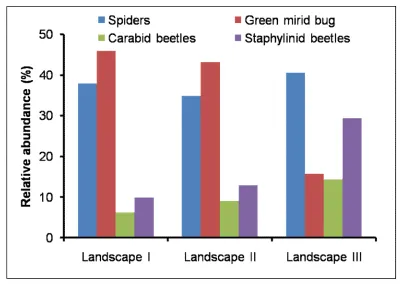
Fig. 7: Relative abundance of four predators in three rice landscapes.
Fig. 8: Empirical variograms in one direction for the RED spectral band of an LANDSAT 8
421
image of 30 m ground spatial distance per pixel, of 6 southern Bangladesh Unions, were
422
sampled for NE abundances.
423
Reference
424
Ahmed N, Islam Z, Hasan M, Kamal NQ, 2002. Effect of Some Commonly Used Insecticides
425
on Yellow Stem Borer Egg Parasitoids in Bangladesh. Bangladesh J Entomol, 12, 37-46.
426
Ahmed N, Englund JE, I Åhman, Lieberg M, Johansson E, 2011. Perception of pesticide use
427
by farmers and neighbours in two periurban areas. Sci. Total Environ, 412, 77–86.
428
BCPA (Bangladesh Crop Protection Association), 2013. List of Registered Agricultural, Bio
429
& Public Health Pesticide in Bangladesh. 142p. http://www.bcpabd.com
430
Bianchi, F., Booij, C.J.H., Tscharntke, T., 2006. Sustainable pest regulation in agricultural
431
landscapes: a review on landscape composition, biodiversity and natural pest control.
432
Proceedings of the Royal Society B: Biological Sciences 273, 1715–1727.
433
Chien HV, Cuong L, 2009. Farms that apply insecticides for leaf folder control are 10 times
434
more at risk to hopperburn. Available: http://ricehoppers.net/2009/09/farms-that
-apply-435
insecticides-for-leaf-folder-control-are-10-times-more-at-risk-to-hopperburn/. Accessed 13
436
Sept 2009.
437
Duveiller G, Defourny P (2010) A conceptual framework to define the spatial resolution
438
requirements for agricultural monitoring using remote sensing. Remote Sens Environ
439
114:2637-2650.
440
Hershey, R.R., 2000. Modeling the spatial distribution of ten tree species in Pennsylvania. In:
441
Mowrer, H.T., Congalton, R.G. (Eds.), Quantifying Spatial Uncertainty in Natural Resources:
442
Theory and Applications for GIS and Remote Sensing. Ann Arbor Press, Chelsea, MI, pp.
443
119–135.
Hassan ASMR, Bakshi K, 2005. Pest Management, productivity and environment: A
445
comparative study of IPM and conventional farmers of Northern Districts of Bangladesh. Pak
446
J Soc Sci, 3, 1007-1014.
447
Heong KL, 2011. Ecological Engineering – a strategy to restore biodiversity and ecosystem
448
services for pest management in rice production. Technical Innovation 11.
449
http://www.spipm.cgiar.org/c/
450
Heong KL, 2010. Assessing BPH outbreak risks of commonly used insecticides. Available:
451
http://ricehoppers.net/2010/09/farmers-in-central-thailand-remain-trapped-by-the-bph-452
problem/. Accessed 30 Sept 2010.
453
Heong KL, 2009. Planthopper outbreaks in 2009. Available: http://ricehoppers.net/2009/09/.
454
Accessed 25 Sept 2009.
455
Heong KL, Schoenly KG, 1998. Impact of insecticides on herbivore-natural enemy
456
communities in tropical rice ecosystems. In: Haskell PT, McEwen P, editors. Ecotoxicology:
457
Pesticides and Beneficial Organisms. Chapman and Hall, London, UK. 381–403.
458
IRRI, 2014. International Rice Research Institute, Philippines
459
(http://ricestat.irri.org:8080/wrs2/entrypoint.htm) accessed on 8 December 2014.
460
Islam Z, Haque SS, 2009. Rice planthopper outbreaks in Bangladesh. Available:
461
http://ricehoppers.net/2009/08/rice-planthopper-outbreaks-in-bangladesh/planthopper-462
outbreaks-in-2009. Accessed 20 Aug 2009.
463
Islam Z, Hossain M, Chancellor T, Ahmed N, Hasan M, Haq M, 2010. Organic
Rice-464
Cropping in Bangladesh: Is it a Sustainable Alternative to Conventional Practice! J Environ
465
Sci Nat Res, 3, 233-238.
466
Levin SA (1992) The Problem of Pattern and Scale in Ecology. Ecology 73:1943-1967.
Luecha M, 2010. Farmers’ insecticide selections might have made their farms vulnerable to
468
hopperburn in Chainat, Thailand. Available:
469
http://ricehoppers.net/2010/01/farmers%e2%80%99. Accessed 17 Jan 2010.
470
Matsumura M, Sanada-Morimura S, 2010. Recent status of insecticide resistance in Asian
471
rice planthoppers. JARQ 44, 225–230. doi: 10.6090/jarq.44.225
472
Moni 2011. BPH continues to threaten Thai rice farmers – heavy losses expected. Available:
473
http://ricehoppers.net/2011/04/bph-continues-to-threaten-thai-rice-farmers
heavy-losses-474
expected/. Accessed 20 April 2011.
475
Moni 2012. Planthopper problems intensify in Thailand’s rice bowl. Available:
476
http://ricehoppers.net/2012/03/planthopper-problems-intensify-in-thailands-rice-bowl/.
477
Accessed 21 March 2012.
478
Rahaman MM, Islam KS, Jahan M, Mamun MAA, 2014. Relative abundance of stem borer
479
species and natural enemies in rice ecosystem at Madhupur, Tangail, Bangladesh. J Bangl
480
Agril Univ, 12, 267–272.
481
482
Shaw, D. R. and Willers, J. L. 2006. Improving pest management with remote sensing.
483
Outlooks on Pest Mgt. 17(5): 197-201.
484
485
Sigsgaard L, 2000. Early season natural biological control of insect pests in rice by
486
spiders - and some factors in the management of the cropping system that may affect this
487
control. In: European Arachnology. Ed. by Toft S, Scharff N, pp. 57-64.
488
489
Soitong K, Sriratanasak W, 2012. Will planthoppers continue to threaten Thailand’s rice
490
production in 2012? Rice Department, Bangkok, Thailand. Available:
http://ricehoppers.net/2012/02/will-planthopper-continue-to-threaten-thailands-rice-492
production-in-2012/. Accessed 13 Feb 2012.
493
Stein, A., van der Meer, F., and Gorte, B, (eds). 2002. Spatial statistics for remote sensing.
494
Kluwer Academic Publishers, Dordrecht, Boston, London.
495
Stern V M, Smith RF, Van Den Bosch R, Hagen KS. 1959. The integrated control concept.
496
Hilgardia, 29, 81-101.
497
Teo C, 2011. Insecticide abuse in rice production causes planthopper outbreaks. Available:
498
http://www.asianscientist.com/topnews/irri-ban-insecticides-rice-production-due-to-499
planthopper-outbreaks-2011/. Accessed 21 Dec 2011.
500
Travisi CM, Nijkamp P, Vindigni G, 2006. Pesticide risk valuation in empirical economics: a
501
comparative approach. Ecol Econ, 56, 455–74.
502
Wang L, Hui C, Sandhu HS, Li Z, Zhao Z, 2015. Population abundance and associated
503
factors of cereal aphids and armyworms under global change. Sci Rep 5, 18801; doi:
504
10.1038/srep18801.
505
Werling, B.P., Meehan, T.D., Robertson, B.A., Gratton, C., Landis, D.A., 2011. Biocontrol
506
Potential Varies with Changes in Biofuel–Crop Plant Communities and Landscape
507
Perenniality. GCB Bioenergy. doi:10.1111/j.1757-1707.2011.01092.x.
508
Willers, J. L., Jenkins, J. N., Ladner, W. L., Gerard, P. D., Boykin, D. L., Hood, K. B.,
509
McKibben, P. L., Samson, S. A., and Bethel, M. M. 2005. Site-specific approaches to cotton
510
insect control. Sampling and remote sensing techniques. Prec. Agric. 6: 431-452.
511
Woltza JM, Isaacsb, R, Landisa DA, 2012. Landscape structure and habitat management
512
differentially influence insect natural enemies in an agricultural landscape. Agricul Ecosyst
513
Environ, 152, 40– 49.
Zhaofei Wen, Wu Shengjun, Liu Feng, Zhang Shuqing, Dale Patricia (2013) Variogram
515
Analysis for Assessing Landscape Spatial Heterogeneity in NDVI: an Example Applied to
516
Agriculture in the Jiansanjiang Reclamation area, Northeast China. Advances in Intelligent
517
Systems Research. doi:10.2991/rsete.2013.122
518
519
520
521
Fig. 1: Map of the Southern part of Bangladesh, for the Barisal Division, where six unions
522
contained the three landscape categories (see text for listing) sampled for insects, while all
523
eighteen unions were employed for variography analyses.
524
Fig. 2: Abundance of spider in three rice landscapes. Means followed by the same letter do
526
not differ significantly at 5% level. The error bar represents the standard error. (***, ** and *
527
indicate significant at 0.1%, 1% and 5% level respectively. Capital and small letters indicate
528
the rice bund and rice plot in different landscapes respectively.)
529
530
531
532
533
534
535
536
537
Fig. 3: Effect of rice bund width on the spider individuals. Ten complete sweeps were used to
539
record population from rice bund.
540
541
542
543
544
545
546
547
548
549
Fig. 4: Abundance of green mirid bug (GMB) in three rice landscapes. Means followed by
551
the same letter do not differ significantly at 5% level. The error bar represents the standard
552
error. (*** indicates significant at 0.1% level. Capital and small letters indicate the rice bund
553
and rice plot in different landscapes respectively.)
554
555
556
557
558
559
560
561
562
Fig. 5: Abundance of carabid beetles (CDB) in three rice landscapes. Means followed by the
564
same letter do not differ significantly at 5% level. The error bar represents the standard error.
565
(*** indicates significant at 0.1%, level. Capital and small letters indicate the rice bund and
566
rice plot in different landscapes respectively.)
567
568
569
570
571
572
573
574
575
Fig. 6: Abundance of staphylinid beetles (STPD) in three rice landscapes. Means followed by
577
the same letter do not differ significantly at 5% level. The error bar represents the standard
578
error. (* indicates significant at 5% level. Capital and small letters indicate the rice bund and
579
rice plot in different landscapes respectively. ns: non-significant at 5% level.)
580
581
582
583
584
585
586
587
588
Fig. 7: Relative abundance of four predators in three rice landscapes.
590
591
592
593
594
595
596
597
598
599
Fig. 8: Empirical variograms in four directions for the RED spectral band of an LANDSAT 8
601
image of 30 m ground spatial distance per pixel, of 6 southern Bangladesh Unions, which
602
were sampled for NE abundances.
603
604
605
606
Angle = 135 Angle = 90
Angle = 45 Angle = 0
0 2000 4000 6000
0 2000 4000 6000
0 100 200 300 400 500 0 100 200 300 400 500
Empirical Semivariogram for ResidualRED
Angle = 135 Angle = 90
Angle = 45 Angle = 0
0 2000 4000 6000
0 2000 4000 6000