On
the
Reynolds-averaged
Navier-Stokes
E
quations
Bohua Sun11
School of Civil Engineering & Institute of Mechanics and Technology, Xi’an University of Architecture and Technology, Xi’an 710055, China
ThispaperattemptstoclarifyanissueaboutthenumberofunknownsintheReynolds-Averaged Navier-Stokesequations(RANS).Thestudydiscoversthatallperspectivesregardingthenumbersof unknownsintheRANSstemsfromthemisinterpretationoftheReynoldsstresstensor.Thecurrent literature considersthat theReynolds stress tensorhas sixunknowns; however, this papershows thattheReynoldsstresstensoractuallyhasonlythreeunknowns,namelythethreecomponentsof fluctuationvelocity. ThetransportequationonboththeReynoldsstresstensorandkineticenergy are discussedaswell. Asapplication,theturbulentBerger’sequationandPrandtlboundarylayer equationsareresolved. Allsolutionshavenoanyadjustableparameters. Thepaperalsoproposea generalalgorithmforthreedimensionalturbulenceflow. Itisfoundthatthemagnitudeofvelocity fluctuationsorturbulenceareproportionaltotheflowpressure,whichisaremarkablediscovery.
Keywords: turbulence; theReynoldsstresstensor; turbulenceclosureproblem
INTRODUCTION
Turbulence is everywhere, controlling the drag on cars, airplanes, and trains, whilst dictating the weath-er through its influence on large-scale atmosphweath-eric and oceanic flows. Even solar flares are a manifestation of turbulence since they are triggered by vigorous motions on the surface of the Sun [1–40].
The study of turbulence is a difficult subject owing to its complex and forbidding mathematical descriptions, which is often considered as the last unsolved problem in classical physics. In 1895 Reynolds published a seminal work on turbulence [1], in which he proposed that flow velocity uand pressurepare decomposed into its time-averaged quantities, ¯u, ¯p, and fluctuating quantities, ˜u, ˜
p; thus, the Reynolds decompositions are:
u = ¯u(x) + ˜u(x, t), (1) p(x, t) = ¯p(x) + ˜p(x, t), (2)
where coordinates and time are (x, t). According to Reynolds, ¯u represent a mean-motion at each point and ˜u a motion at the same point relative to the mean-motion at the point. Therefore, the Reynolds called the ¯u mean-motion and ˜u relative-mean-motion [1]. The time-averaging definition is given by ¯u(x) = limT→∞T1
∫t0+T
t0 u(x, t)dt, and time-fluctuation ˜u=u− ¯
u(x).
REYNOLDS-AVERAGED NAVIER-STOKES EQUATIONS
With the decomposition the Navier-Stokes equa-tion is then transformed into the Reynolds-averaged
Navier–Stokes equations (RANS) as follows
ρ∇·( ¯u⊗u¯) +∇p¯ = µ∇2u¯+∇·τ, (3)
∇·u¯ = 0, (4)
where dynamic viscosityµ, gradient operator∇=ei∇i,
base vector in the i-coordinateei, and tensor product⊗,
and the Reynolds stress tensor is given by
τ =−ρu˜⊗u˜=−ρ lim
T→∞
1 T
∫ t0+T
t0
( ˜u⊗u˜)dt, (5)
where T is the period of time over which the averaging takes place and must be sufficiently large to give mean-ingful averages and is needed to measure mean values depends on the accuracy desired. Reynolds stress is ap-parent stress owing to the fluctuating velocity field ˜u.
Denoting kinematic viscosityν=µ/ρ, the above equa-tions can be equivalently rewritten in conventional form:
¯
u·∇u¯+1
ρ∇p¯+ limT→∞
1
T ∫t+T
t ( ˜u·∇u˜)dt
=ν∇2u,¯ (6)
∇·u¯= 0 (7)
HOW MANY UNKNOWNS ARE THERE IN THE RANS ???
All current literatures and textbooks believe that the Reynolds stresses τ has six unknowns (In the later, we will show that the Reynolds stresses have only three un-knowns instead of six ones.). This understanding result-s a conresult-senresult-suresult-s of result-saying that there are 10 unknownresult-s in Eqs.3, 4 and/or Eqs.35, 35.
If you carefully read Reynolds’ paper in 1895 [1], and will see that Reynolds did not discussed the number of unknowns in the RANS. However, from his presentation we are sure that he never considered the termρu˜⊗u˜ as
independent unknowns, while for some cases he even pro-posed explicit expressions for the velocity fluctuation ˜u, for instance, expressions in page 149 and Eq.(50) in page 158 of Reynolds paper [1], which means that he actually take the velocity fluctuation ˜uas unknowns. Due to the limited references, the author has no idea who was the first person proposed this 10-unknowns perception on the RANS.
Clearly, the RANS in Eqs.3, 4 has four independent equations governing the mean velocity field; namely the three components of the Reynolds equation Eqs.3 togeth-er with the mean continuity equation Eq.4. Howevtogeth-er, these four equations contain more than four unknowns. In addition to ¯uand ¯p, there are also the Reynolds stress-esτ, which results the Reynolds-averaged Navier-Stokes equations unclosed. The closure problem is being consid-ered as the number one topic in turbulence, during the past several decades, scientists and engineers have made many attempts towards solving the closure problem.
Regarding the RANS closure problem, the curren-t consensus is curren-thacurren-t curren-there are six unknown componencurren-ts in the symmetric Reynolds stress tensor τ, namely τ11, τ12, τ13, τ22, τ23, τ33. However, we have a complete-ly different perspectives. What we believe is that the Reynolds stress tensorτ has only three unknowns, name-ly the velocity fluctuation componentsu′i(i= 1,2,3) due to the fact that the Reynolds stress tensor is simply an integration of a second order dyadic tensor of flow veloc-ity fluctuations rather than a general symmetric tensor.
LEMMAS
To support our statement, let’s us introduce some lem-mas as follows
Lemma 1 Giving two vectors, v(x, t) = viei =v1e1+
v2e2+v3e3 andw(x, t) =wjej=w1e1+w2e2+w3e3,
we can defined a dyadic tensor v⊗w as follows [41]
v⊗w=viei⊗wjej=viwjei⊗ej
=v1w1e1⊗e1+v1w2e1⊗e2+v1w3e1⊗e3 +v2w1e2⊗e1+v2w2e2⊗e2+v2w3e2⊗e3 +v3w1e3⊗e1+v3w2e3⊗e2+v3w3e3⊗e3.
(8) In general case ofv̸=w, the dyadic tensorv⊗wis a general tensor with 9 components (elements),and have 6 unknowns, namely, v1, v2, v3 and w1, w2, w3, since the 9 components can be fully determined by the 6 unknowns.
If v=w, the tensor v⊗w is a 2rd order tensor with
9 components (elements), and have 3 unknowns, namely, v1, v2, v3and/orw1, w2, w3, since the 9 components can be fully determined by the 3 unknowns.
Lemma 2 Giving three vectors,u(x, t) =uiei=u1e1+
u2e2+u3e3 , v(x, t) = viei = v1e1+v2e2+v3e3 and
w(x, t) =wjej =w1e1+w2e2+w3e3, we can defined a
3rd order tensorv⊗w as follows
u⊗v⊗w=uiek⊗vkei⊗wjej =ukviwjek⊗ei⊗ej.
(9)
In general case of u̸=v ̸=w, the tensor u⊗v⊗w is a general tensor with 27 components (elements), and have 9 unknowns, namely, u1, u2, u3, v1, v2, v3 and w1, w2, w3, since the 27 components can be fully deter-mined by the 9 unknowns.
Ifu=v=w, the tensoru⊗v⊗wis a 3rd order tensor
with 27 components (elements), and have 3 unknowns, namely, u1, u2, u3, or v1, v2, v3 and/or w1, w2, w3, s-ince the 27 components can be fully determined by the 3 unknowns.
Lemma 3Giving a vector, v(x, t) = viei = v1e1 + v2e2+v3e3, we can defined a 2nd order symmetric dyadic tensorv⊗v and its mean valueA(x)as follows
A(x) = lim
T→∞
1 T
∫ t0+T
t0
v⊗vdt
= lim
T→∞
1 T
∫ t0+T
t0
vivjei⊗ejdt
= lim
T→∞
1 T
∫ t0+T
t0
[v1v1e1⊗e1+v1v2e1⊗e2
+v1v3e1⊗e3+v2v1e2⊗e1 +v2v2e2⊗e2+v2v3e2⊗e3 +v3v1e3⊗e1+v3v2e3⊗e2
+v3v3e3⊗e3]dt (10)
where vivj =vjvi. Although A(x) has six
independen-t componenindependen-ts,namely v1v1, v1v2, v1v3, v2v2, v2v3, v3v3, however it is clear there are only three independent quan-tities, namely, v1, v2, v3, in the A(x). It is because that the quantities v1v1, v1v2, v1v3, v2v2, v2v3, v3v3 can be fully determined byv1, v2, v3.
The lemma 3 actually states that any (time) averaging operation is just a method of data processing and will not change the number of unknowns of the problem.
It is clear thatA(x) will be the Reynolds stress tensor τ, if replacing v1, v2, v3 by the components of velocity fluctuations ˜ui(i = 1,2,3), respectively, namely, v1 = ˜
u1, v2= ˜u2, v3= ˜u3.
PROOF 1
be defined by
τ =−ρu˜⊗u˜
=−ρu˜iei⊗u˜jej =−ρu˜iu˜jei⊗ej
=−ρ lim
T→∞
1 T
∫ t0+T
t0
(˜uiu˜jei⊗ej)dt
=
[
−ρ lim
T→∞
1 T
∫ t0+T
t0 ˜ uiu˜jdt
]
ei⊗ej
=τijei⊗ej, (11)
and the fluctuation velocity convective terms are given by:
˜
u·∇u˜= ˜uiei·[ek∂k⊗(˜ujej)]
= ˜uiu˜j,kei·(ek⊗ej) = ˜uiu˜j,k(ei·ek)ej
= ˜uiu˜j,kδikej= ˜uiu˜j,iej
= ( lim T→∞ 1 T
∫ t+T
t
˜ uiu˜j,idt
) ej
=τij,iej, (12)
where the Reynolds stress tensor in index format τij is
defined by
τij =τji=−ρ lim T→∞
1 T
∫ t0+T
t0 ˜
ui˜ujdt. (13)
It is clear that anyτijcan be calculated by fluctuation
ve-locity components ˜u1,u2,˜ u3˜ , which means that the τij
are dependent on the components ˜u1,u2,˜ u3˜ . In other words, the components ˜u1,u2,˜ u3˜ are real unknowns. It is the key point why we say that the Reynolds stress ten-sorτ has 6 unknowns is a big mistake in the turbulence modelling.
Therefore, the formulation in Eq.11 reveals that the Reynolds stress tensor τ = −ρu˜⊗u˜ can be fully cal-culated by three independent components of fluctuation velocity ˜u1,u2,˜ u3˜ . In other words, the Reynolds stress tensor has only three unknowns rather than six ones. It means that the averaging technique is just a math-ematical processing, which can provide us a mean value, however, can’t change the number of unknowns of the problem.
The misinterpretation regarding the numbers of un-known components of all literature may stem from con-sidering the Reynolds stress tensor as a general 2nd or-der symmetric tensor with six independent components. However, the Reynolds stress tensor is not an arbitrary 2nd order tensor, actually each of its component is made by the bi-product of fluctuation velocity components, which means that the Reynolds stress tensor is an dyadic tensor of the velocity fluctuation. The unknown nents to construct the dyadic tensor are the three compo-nents of fluctuation velocity ˜u. Therefore, the Reynolds
stress tensor has only three unknowns, namely ˜u1,u2,˜ u3˜ . For two dimensional flow, of course, the 2D Reynolds stress tensor has only two unknowns, namely ˜u1,u2˜ .
PROOF 2
Given two scalar functions, ˜u=√2Ucos(ωt) and ˜v =
√
2V cos(ωt+θ), as independent unknowns, we can use them to construct a 2nd order tensor or matrix with 4 components as follows: (˜u)2,u˜˜v,˜vu,˜ (˜v)2.
Thus time averages give:
lim
T→∞
1 T
∫ t0+T
t0
(˜uu˜)dt = U2 (14)
lim
T→∞
1 T
∫ t0+T
t0
(˜uv˜)dt = U Vcosθ (15)
lim
T→∞
1 T
∫ t0+T
t0
(˜vu˜)d = U Vcosθ (16)
lim
T→∞
1 T
∫ t0+T
t0
(˜vv˜)dt = V2 (17)
In the definition of the Reynolds stress tensor,θ= 0, we have ˜u = √2Ucos(ωt) and ˜v = √2V cos(ωt) and their averaging
lim
T→∞
1 T
∫ t0+T
t0
(˜uu˜)dt = U2 (18)
lim
T→∞
1 T
∫ t0+T
t0
(˜u˜v)dt = U V (19)
lim
T→∞
1 T
∫ t0+T
t0
(˜vu˜)dt = U V (20)
lim
T→∞
1 T
∫ t0+T
t0
(˜v˜v)dt = V2 (21)
Therefore, the Reynolds stress tensor is given by
τ =−ρ(U2e1⊗e1+U Ve1⊗e2
+V Ue2⊗e1+V2e2⊗e2). (22) The above process shows that, ˜uor U, and ˜v or V, are the independent unknowns, with them we can get the Reynolds stress tensorτ.
If keeping the θ, namely, then we are talking about the time correlation (autocorrelations) at the same point. The correlation between the same (Greek autos = self or same) fluctuating quantity measured at two different times (at the same point in space) is not itself very rele-vant to the behaviour of turbulence and its measurement requires a time delay mechanism (usually a tape recorder with movable heads or a digital sample-and-delay sys-tem).
Reynolds stress tensor is the one-point or single-point velocity fluctuation correlation. Therefore,θ= 0.
Even not setting θ = 0, the Reynolds stress still has three independent unknowns, namely the three compo-nents of velocity fluctuations. This is the key point of this article. The conclusion of saying that the RANS has only 7 independent unknowns is still correct.
PROOF 3
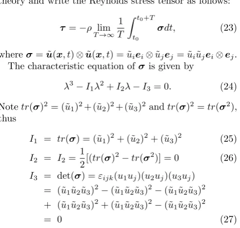
To support this obvious statement from other point of view, let’s study the problem by tensor representation theory and write the Reynolds stress tensor as follows:
τ =−ρ lim
T→∞
1 T
∫ t0+T
t0
σdt, (23)
whereσ= ˜u(x, t)⊗u˜(x, t) = ˜uiei⊗u˜jej = ˜uiu˜jei⊗ej.
The characteristic equation ofσis given by
λ3−I1λ2+I2λ−I3= 0. (24) Notetr(σ)2= (˜u1)2+ (˜u2)2+ (˜u3)2andtr(σ)2=tr(σ2), thus
I1 = tr(σ) = (˜u1)2+ (˜u2)2+ (˜u3)2 (25) I2 = I2= 1
2[(tr(σ)
2−tr(σ2)] = 0 (26) I3 = det(σ) =εijk(u1uj)(u2uj)(u3uj)
= (˜u1u2˜ u3˜ )2−(˜u1u2˜ ˜u3)2−(˜u1u2˜ u3˜ )2 + (˜u1u2˜ u3˜ )2+ (˜u1u2˜ ˜u3)2−(˜u1u2˜ u3˜ )2
= 0 (27)
Therefore, the characteristic equation of σ in Eq.23 has three roots as follows
λ1= 0, λ2=I1, λ3= 0. (28) From spectra representation theory of a symmetric ten-sor, we can rewrite the tensorσ as follows
σ=λ1ˆe1⊗ˆe1+λ2eˆ2⊗ˆe2+λ3ˆe3⊗ˆe3
=λ2ˆe2⊗ˆe2, (29)
where the base ˆei is an eigenvector of σ, which can be
determined by eigenvalue equation
σ·ˆe= 2kˆe·ˆe (30)
where the fluctuation kinetic energyk= 12[(˜u1)2+(˜u2)2+ (˜u3)2], we find
ˆ
e2=√1
2ku˜ℓeℓ (31) Hence we have
σ= [(˜u1)2+ (˜u2)2+ (˜u3)2]ˆe2⊗ˆe2, (32)
Therefore, the Reynolds tress tensor can be also given by
τ =−ρ lim
T→∞
1 T
∫ t0+T
t0
σdt
=−ρ lim
T→∞
1 T
∫ t0+T
t0
[(˜u1)2+ (˜u2)2+ (˜u3)2]ˆe2⊗ˆe2dt. (33)
It is proved once again that both the tensor σ and the Reynolds stress tensor τ are the only function of ˜
u1,u˜2,u˜3. As a summary, the number of unknowns of the Reynolds stress tensor is listed in the Table II:
TABLE I: Numbers of unknowns in the Reynolds stress Current literatures This paper
Numbers 6 3
Unknowns τ11, τ12, τ13, τ22, τ23, τ33 u˜1,u˜2,˜u3
Although the Reynolds-averaged Navier-Stokes (RAN-S) equations are unclosed, however, the four-equations RANS in Eqs.3 and 4 contain only 7 unknowns instead of 10 ones. The list of unknowns in the RANS are sum-marized in the below Table II:
TABLE II: Numbers of unknowns in the RANS Current literature This paper
Numbers 10 7
Unknowns u¯1,u¯2,u¯3 u¯1,u¯2,¯u3 ¯
p p¯
τ11, τ12, τ13, τ22, τ23, τ33 u˜1,u˜2,˜u3
In the future, turbulence modelling will be focus on velocity fluctuations ˜u1,u˜2,u˜3 instead of the Reynolds stressτij. Advantage of modelling the velocity
fluctua-tions ˜u1,u˜2,u˜3 is obvious, since it reduce the 6 compo-nents of τij into 3 components of velocity fluctuations,
and from experimental point of view, the components of velocity fluctuations are easy to be measured than the Reynolds stress tensor.
TRANSPORT EQUATION OF REYNOLDS STRESS TENSOR
With the above new understanding on the number of unknowns. In the following, we will present complete new perception on the higher-order correction of the Reynolds stress tensor.
tensorial form as follows
ρu˜,t+ρ∇·( ¯u⊗u˜+ ˜u⊗u¯+ ˜u⊗u˜) +∇p˜ (34)
=µ∇2u˜+ρlim
T→∞T1 ∫t+T
t ∇·( ˜u⊗u˜)dt,
∇·u˜ = 0. (35)
According to the author’s investigations [38–40], Eqs.3, 3, 3, and 3 form a closed integral-differential equations system, in which there are 8 equations with 8 unknowns
¯
u,u,˜ p,¯ p˜.
After some tensor algebra we arrive at an important equation on the Reynolds stress tensor as follows
∂τ
∂t + ¯u·∇τ =−τ·∇u¯−∇u¯·τ +2µI:∇u˜⊗∇u˜+ ˜u⊗(∇p˜) + (∇p˜)⊗u˜
+µ∇2τ+ρ∇·( ˜u⊗u˜⊗u˜). (36) In current literature, it is believe that Eq.36 has 31 un-knowns. However, we have complete different opinion. We believe the Reynolds stress equation Eq. 36 has only 7 unknowns. Specifically, accoutring for all symmetries, we have the following listed in the Table III.
TABLE III: Numbers of unknowns in the Reynolds stress e-quation
Current literature This paper
Numbers 31 7
Unknowns u¯ (3) u¯1,u¯2,¯u3 ˜
u⊗u˜⊗u˜ (10) p˜ I:∇u˜⊗∇u˜(6) u˜1,u˜2,˜u3
˜
u⊗(∇p˜) (6) τ (6)
The above statement can be easily proved. For in-stance,
˜
u⊗u˜⊗u˜= ˜uiu˜ju˜kei⊗ej⊗ek
= [ lim
T→∞
1 T
∫ t0+T
t0
(˜uiu˜ju˜k)dt]ei⊗ej⊗ek, (37)
and
I:∇u˜⊗∇u˜= (ek⊗ek) : (∇u˜⊗∇u˜)
= (ek⊗ek) : (∇u˜⊗∇u˜) = (ek·∇u˜)⊗(ek·∇u˜)
= (∇ku˜)⊗(∇ku˜) = (∇ku˜iei)⊗(∇ku˜jej)
= (∇ku˜i)(∇ku˜j)ei⊗ej=
∂u˜i
∂xk
∂u˜j
∂xk
ei⊗ej
= [ lim
T→∞
1 T
∫ t0+T
t0
(∂u˜i ∂xk
∂u˜j
∂xk
)dt]ei⊗ej.
(38)
It is clear that mean value of ˜uiu˜ju˜k and ∂x∂u˜i
k
∂˜uj
∂xk can be calculated by the velocity fluctuations ˜u1,u2,˜ u3˜ . It
means that ˜u1,u2,˜ u3˜ are unknowns. Similarly,
˜
u⊗(∇p˜) = ˜ui
∂p˜ ∂xj
ei⊗ej
= [ lim
T→∞
1 T
∫ t0+T
t0 (˜ui
∂p˜ ∂xj
)dt]ei⊗ej. (39)
The mean value of ˜ui∂x∂p˜
j can be calculated by ˜p and ˜
u1,u2,˜ u3˜ .
In the same way, we can still do the fourth order and higher orders as in [4] and textbooks. However, there is no more unknowns can be created by any order equation about the Reynolds stress tensor.
TRANSPORT EQUATION OF TURBULENCE KINETIC ENERGY
If we do contraction operation for index i and j in the Eq.36, we have following transport equation for the turbulence kinetic energyk
ρ(∂k
∂t + ¯u·∇k) =τ :∇u¯−µ∇u˜:∇u˜ +µ∇2k−∇·(˜pu˜)−1
2ρ∇·[( ˜u·u˜) ˜u] (40) where the kinetic energyk=−12τkk = 12u˜ku˜k = 12u˜·u˜.
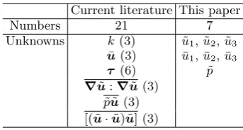
The number of unknowns in the kinetic energy equation Eq.40 is listed in the Table IV.
TABLE IV: Numbers of unknowns in the kinetic energy equa-tion
Current literature This paper
Numbers 21 7
Unknowns k(3) u˜1,u˜2,u˜3 ¯
u(3) u¯1,u¯2,u¯3 τ (6) p˜
∇u˜:∇u˜(3) ˜
pu˜ (3) [( ˜u·u) ˜˜ u] (3)
In order to support the above understanding about the number of unknowns, let’s present some examples in the following. The aim of doing these exercise are only for demonstration purpose: to show general algorithm to find turbulence solutions. We will not going to give complete solutions here, so that we can stay on our key focus, namely, to determine the number of unknowns in the Reynolds-averaged Navier-Stokes equations.
EXAMPLE 1: ONE DIMENSIONAL BERGER’S EQUATION
One dimensional Navier-Stokes equation, namely, Bergers’s equation
where the source termS(x, t) is given by S(x, t) = cos(x+t) +νsin(x+t)
+Bcos(x+t) tanh(A− B 2νx) + sin(x+t) cos(x+t)
− 1
2νB
2sin(x+t)[1−tanh2 (A− 1
2νBx)], (42) where the trigonometric tangent function is defined as tanh(x) = sinh(cosh(xx))= eexx+−ee−−xx, andA, B are constant.
Substituting the Reynolds velocity decompositionu= ¯
u(x)+ ˜u(x, t) into Eq.41, after time-averaging, we can get its RANS as follows
¯
uu¯,x+ ˜uu˜,x=νu¯,xx+ ¯S, (43)
namely
¯
u¯u,x+ lim T→∞
1 T
∫ t0+T
t0 ˜
uu˜,xdt=νu¯,xx+ ¯S, (44)
where the mean source term ¯S= 12. Obviously, the Eq.44 has only two unknowns, one is the mean velocity ¯uand another is velocity fluctuation ˜u, as stated in the previous part.
Since we have only one integral-differential equation Eq.44, therefore, the Eq.44 is not closed. To solve the Eq.44, we have to model either the mean field ¯uor fluc-tuation ˜u.
We can use the steady solution of ¯uu¯,x=νu¯,xxas the
1st order approximate solution of mean field. Hence, the 1st order exact solution is given by
¯
u(x) =B1tanh(A1− B1
2νx), (45) where the constantsA1, B1will be determined later.
For fluctuation field ˜u, since its mean ˜umust be zero, namely, limT→∞T1
∫t0+T
t0 udt˜ ≡0, hence, we can take the 1st order velocity fluctuation proposed by Reynolds [1] as an approximate solation
˜
u(x, t) =√2asin(ωt+κx), (46) where a, frequencyω and wave number κare to be de-termined.
Substituting both Eqs.45 and 46 into Eq.44, we obtain
a=√1
2κ (47)
Therefore, we have the 1st order velocity field as follows
u(x, t) =B1tanh(A1− B1 2νx) +
1
√
2κsin(ωt+κx). (48) For initial-boundary conditionsu(0,0) = 1, u,x(0,0) = 1,
we get B1 = √1 +ν, tanh(A1) = √1
1+ν u,t(0,0) =
1, u,xx(0,0) = 1, and obtain ω =
√
κ and κ =
1+ν+√1+ν
2ν2 −1.
Hence, the 1st order solution is obtained
u(x, t) =√1 +νtanh(A1−
√
1 +ν 2ν x) +√1
2κsin(
√
κt+κx). (49)
(1) The 1st order turbulence velocity u1st is different
from the exact solution of the Bergers equation in Eq.41. The exact solution of Berger’s equation is given by
uexact(x, t) =Btanh(A−
B
2νx) + sin(x+t). (50) (2) In particular, when x→ ∞, their asymptotic be-havior are totally different. The exact solution is going to be uexact = B+ sin(x+t), due to the property of
limx→∞tanh(x)→1, while the turbulence solution
u(x, t) =√1 +ν+√1 2κsin(
√
κt+κx).. (51)
(3) The turbulence kinetic energy is given by k = 1/(2κ)
For a better approximation, the velocity fluctuations can be assumed as ˜u(x, t) =√2a(x) sin(ωt).
EXAMPLE 2: TURBULENT BOUNDARY LAYER FLOW OF SEMI-INFINITE SURFACE
Here velocity components u = u1, v =u2, directions 1→x,2→yare adopted respectively.
According to Prandtl’s boundary layer concept [2, 42], the two dimensional Navier-Stokes equations can be sim-plified to following boundary layer equations
u,t+uu,x+vu,y=U
dU
dx +µu,yy, (52)
u,x+v,y= 0, (53)
whereU(x) is incoming velocity, U =const. for infinite surface, henceU,x= 0.
In duct and boundary layer flow, we can approximate with excellent accuracy a simpler turbulent boundary layer equations
ρ(¯uu¯,x+ ¯vu¯,y) =U
dU
dx +τxx,x+τxy,y, (54) ¯
u,x+ ¯v,y= 0, (55)
where total stress
τxx=−ρu˜u˜=−ρ lim T→∞
1 T
∫ t0+T
t0 ˜
uudt,˜ (56)
τxy=µu¯,y−ρu˜˜v=µu¯,y−ρ lim T→∞
1 T
∫ t0+T
t0 ˜
To solve the above equations, we firstly omit the fluctu-ation term and reduce Eqs.54 and 55 into followings
ρ(¯uu¯,x+ ¯vu¯,y) =µu¯,yy, (58)
¯
u,x+ ¯v,y= 0, (59)
Blasius [42] has obtained their solutions as follows ¯
u=U f′(ξ), (60)
¯ v=1
2
√ νU
x (ξf
′−f), (61)
where ξ =y √
U
νx, U is incoming velocity, f′ = df dξ, and
functionf(ξ) is the solution of equationf f′′+ 2f′′′ = 0 under conditionsf(0) =f′(0) = 0, f′(∞) = 1.
For fluctuation field ˜uand ˜v, since their mean must be vanish, hence, we can take the 1st order velocity fluctu-ation suggested by Reynolds [1] as their solutions
˜
u=√2c1cos(φ), (62) ˜
v=√2c2cos(φ), (63) where phase functionφ=ωt+κxx+κyy, and constants
c1, c2.
Substituting Eqs. 60,61,62 and 63 into Eq. 54, we obtain
(c21)κx+ (c1c2)κy=U
dU
dx = 0. (64)
to determine c1, c2, we need mass conversation law of fluctuation field ˜u,x+ ˜v,y = 0, namely κx =−κy = κ,
find thec1=c2=C, hence, we can write down velocity field as follows
u=U f′(ξ) +√2Ccos(ωt+κx−κy), (65)
v=1 2
√ νU
x (ξf
′−f) +√2Ccos(ωt+κx−κy), (66)
where frequencyω, wave number κand constant C can be determined by 3 initial-boundary conditions.
In the future, for a better approximation, we can take ˜
u=√2c1(x, y) cos(ωt) and ˜v=√2c2(x, y) cos(ωt). We must point out here that the one and/or two di-mensional Navier-Stokes model can not represent a real turbulence, since turbulence motion is always three di-mensional [7].
EXAMPLE 3: THREE DIMENSIONAL TURBULENT FLOW SOLUTION ALGORISM
Although there are different views about turbulence, there is a consensus that the deterministic Navier-Stokes equation probably contains all information, which is rel-evant to turbulence [18].
For three dimensional turbulent flow, we propose fol-lowing algorithm:
(1) Find solution of corresponding equations of steady flow ¯u:
∇·( ¯u⊗u¯) =ν∇2u.¯ (67)
(2) Calculate pressure (source term) ¯p:
∇2p¯=−ρ∇·( ¯u·∇u¯). (68)
(3) Propose an approximate solution for velocity fluctu-ations ˜u:
˜
u=√2C(x) cos(ωt). (69) (4) Calculate the Reynolds stress tensorτ:
τ =−ρ lim
T→∞
1 T
∫ t+T
t
( ˜u⊗u˜)dt (70) =−ρ(C⊗C).
(5) Determine the coefficient vector an: Substitute
¯
u,p,¯ τ into the RANS, hence we have
∇·( ¯u⊗u¯)−ν∇2u¯=−1
ρ∇p¯−∇·(C⊗C). (71) Since ¯uis the solution of∇·( ¯u⊗u¯) =ν∇2u¯, therefore, the left side of the above equation is zero, hence
∇·(C⊗C+1
ρpI¯ ) = 0, (72) This relation reveals that the fluctuation magnitude is proportional to pressure, the turbulence can not main-tained without continua source supplying.
(6) Calculate pressure fluctuation ˜p
∇2 ˜
p=−ρ∇·[ ¯u·∇u˜+ ˜u·∇u¯+ ˜u·∇u˜]−τ. (73) (7) Calculate total pressurep:
p= ¯p+ ˜p. (74)
(8) Calculate total velocity fieldu
u= ¯u+C(x) cosωt. (75) In the similar way, you can get higher order solutions.
CONCLUSIONS
but also discovered the number of unknowns is much less than the conventional accoutring.
As application of this study, we have resolved the Berg-er’s equation and turbulent Pranddtl boundary layer e-quations. All solutions have no any adjustable param-eters. It is found that the Reynolds stress is mainly depends on the source term (ie. flow pressure), which means that the turbulence can not maintained if there is no source supplying.
Although the Reynolds-Averaged Navier-Stokes-Equations (RANS) has been formulated for more 100 years, unfortunately, all current literature have a wrong understanding on the numbers of unknowns. This situation must be corrected immediately, otherwise, it will be very harmful to scientific environment and definitely obstructing the understanding and solving of turbulence phenomena. The ideas and methodology of this paper are also applicable to the compressible turbu-lence Navier-Stokes equations. The study in the paper might shed a light to understand the well-known closure problem of turbulence, and will help to understand the puzzle and modelling of turbulence closure problem that has eluded scientists and mathematicians for centuries.
Acknowledgements
It is my great pleasure to have shared and discussed some of the above with Michael Sun from Bishops Dioce-san College, whose pure and direct scientific sense in-spired me.
[1] O. Reynolds, On the dynamical theory of incompress-ible viscous fluids and the determination of the criterion. Philos. Trans. R. Soc. 186:123–164(1895).
[2] L. Prandtl, On fluid motions with very small friction (in German). Third International Mathematical Congress, Heidelberg. 484-491(1904).
[3] L. Prandtl, Bericht uber die entstehung der turbulenz. Z. Angew. Math. Mech 5, 136(1925).
[4] P-Y. Chou, On velocity correlations and the solutions of the equations of turbulent fluctuation. Q. Appl. Math. 111(1):38-54(1945).
[5] P-Y. Chou and R.L. Chou, 50 years of turbulence re-search in China. Annu. Rev. Fluid Mech.27:1-15(1995). [6] P. Bradshaw,An Introduction to Turbulence and Its
Mea-surement. Pergamon Press, New York (1971).
[7] H. Tennekes and J.L. Lumley,A First Course in Turbu-lence. Cambridge: The MIT Press (1972).
[8] D.C. Lesilie,Developments in the Theory of Turbulence. Clarendon Press, Oxford (1973).
[9] A.A. Townsend,The Structure of Turbulent Shear Flow
2nd ed., Cambridge University Press, New York (1976). [10] S.Y. Chen and P.-Y. Zhou, The application of
quasi-similarity conditions in turbulence modeling theory. Journal of Hydrodynamics, 2(2) (1987)
[11] M. Lesieur,Turbulence in Fluids. 2nd ed. Kluwer, Dor-drecht (1990).
[12] D.C. Wilcox,Turbulence Modeling for CFD. D C W In-dustries (1993).
[13] S.B. Pope,Turbulent Flows. Cambridge University Press, Cambridge (2000).
[14] P.A. Davidson, Turbulence. Oxford University Press, Oxford (2004).
[15] B. Hof, Experimental Observation of Nonlinear Traveling Waves in Turbulent Pipe Flow. Science305, 1594 (2004). [16] G. Falkovich and K.R. Sreenivasan, Lessons from hydro-dynamic turbulence. Physics Today, 43-49 (April 2006). [17] C.B. Lee and J.Z. Wu, Transition in wall-bounded flows.
Applied Mechanics Reviews, 61(3), 030802 (2008) [18] U. Frisch,Turbulence: The Legacy of A.N. Kolmogorov.
Cambridge University Press,Cambridge (2008).
[19] I. Marusic, R. Mathis and N. Hutchins, Predictive mod-el for wall-bounded turbulent Flow. Science 329, 193 (2010).
[20] A.J. Smits, B.J. McKeon and I. Marusic, High–Reynolds Number Wall Turbulence, Annu. Rev. Fluid Mech.43, 353 (2011).
[21] P.A. Davison,et al. A Voyage Through Turbulence. Cam-bridge: Cambridge University Press (2011).
[22] B. Suri, J.R. Tithof, R.O. Grigoriev and M.F. Schatz, Forecasting Fluid Flows Using the Geometry of Turbu-lence. Phys. Rev. Lett.118, 114501 (2017).
[23] D. Castelvecchi, On the trial of turbulence. Nature, 548:382 (2017).
[24] L.D. Landau and E. M. Lifshitz, Mechanics (3rd ed.) (Butterworth-Heinemann, Oxford, 1976).
[25] A.N. Kolmogorov, The local structure of turbulence in incompressible viscous fluid for very large Reynold-s number. Dokl. Akad. Nauk SSSR, 30:299-303 (1941a) (reprinted inProc.R.Soc.Lond.A, 434,9-13, 1991). [26] A.N. Kolmogorov, On degeneration (decay) of
isotrop-ic turbulence in an incompressible visous liquid. Dokl. Akad. Nauk SSSR,31:538-540 (1941b).
[27] A.N. Kolmogorov, Dissipation of energy in locally isotropic turbulence. Dokl.Akad. Nauk SSSR, 32 :16-18 (1941c).(reprinted in Proc.R.Soc.Lond. A, 434,15-17, 1991).
[28] K.R. Sreenivasan, On the scaling of the turbulence en-ergy dissipation rate. Physics of Fluids, 27,5:1048-1051 (1984).
[29] Z.S. She and E. L´evˆeque, Universal scaling laws in fully developed turbulence. Phys. Rev. Lett.72,336(1994) . [30] E.N. Lorenz, Deterministic non-periodic flow. J. Atmos
Sci.20:130–41(1963).
[31] R. Benzi, P. Paladin, G. Parisis and A. Vulpiani, On the multifractal nature of fully developed turbulence and chaotic systems. J. Phys. A: Math. Gen. 17 :3521-3531(1984).
[32] S.A. Orszag and G.S. Patterson, Numerical simulation of three-dimensional homogeneous isotropic turbulence. Phys. Rev. Lett.28,76(1972).
[33] B. Sun, The temporal scaling laws of compressible turbu-lence. Modern Physics Letters B.30,(23) 1650297 (2016). [34] B. Sun, Scaling laws of compressible turbulence. Appl.
Math. Mech.-Engl. Ed.38: 765(2017).
[36] B. Sun, A additive decomposition of veloci-ty gradient, Physics of Fluids 31, 061702(2019); doi:10.1063/1.5100872.
[37] B. Sun, On the Reynolds-averaged Navier-Stokes equa-tions, Preprints, doi:10.20944/preprints201907.0038.v1. [38] B. Sun, On closure problem of incompressible
turbulent flow. Preprints 2018, 2018070622 (doi: 10.20944/preprints201807.0622.v2).
[39] B. Sun, An Intrinsic Formulation of Incompress-ible Navier-Stokes Turbulent Flow. Preprints 2018,
2018080071 (doi: 10.20944/preprints201808.0071.v3). [40] Sun, B. A Novel Simplification of the
Reynolds-Chou-Navier-Stokes Turbulence Equations of Incom-pressible Flow. Preprints 2018, 2018070030 (doi: 10.20944/preprints201807.0030.v1).
[41]https://en.wikipedia.org/wiki/Dyadic_tensor [42] H. Blasius, Grenzschichten in Fljssigkeiten mit kleiner