Kinetic Modelling at the Basis of Process Simulation for Heterogeneous Catalytic Process Design

Review

Kinetic Modelling at the Basis of Process Simulation

for Heterogeneous Catalytic Process Design

Antonio Tripodia_{, Matteo Compagnoni}a_{, Rocco Martinazzo}a_{, Gianguido Ramis}b _{and Ilenia} Rossettia,*

a _{Dip. Chimica, Università degli Studi di Milano, CNR-ISTM and INSTM Unit Milano-Università, Milan,}

Italy

b _{Dip. Ing. Chimica, Civile ed Ambientale, Università degli Studi di Genova and INSTM Unit Genova,}

Genoa, Italy

* _{Corresponding author: fax +39-02-50314300; email [email protected]}

ABSTRACT: Process simulation represents an important tool for plant design and optimisation, either applied to well established or to newly developed processes. Suitable thermodynamic packages should be selected in order to properly describe the behaviour of reactors and unit operations and to precisely define phase equilibria. Moreover, a detailed and representative kinetic scheme should be available to predict correctly the dependence of the process on its main variables. This review points out some models and methods for kinetic analysis specifically applied to the simulation of catalytic processes, as a basis for process design and optimisation. Attention is paid also to microkinetic modelling and to the methods based on first principles, to elucidate mechanisms and calculate thermodynamic and kinetic parameters. Different case histories support the discussion. At first, we have selected two basic examples from the industrial chemistry practice, e.g. ammonia and methanol synthesis, which may be described through a relatively simple reaction pathway. Then, a more complex reaction network is deeply discussed to define the conversion of bioethanol into syngas/hydrogen or into building blocks, such as ethylene.

Keywords: process simulation; kinetic modelling; ammonia; methanol; bioethanol; steam reforming; ethylene

1. Implementation of Kinetic Models into Process Simulators

The implementation of kinetic models into process simulators is a scientific and industrial field in continuous growth. Process simulators allow the detailed design of chemical processes with the direct comparison of different scenarios: alternative process layout, size, connection between process streams and equipment are allowed. Through these instruments, it is possible to size and optimise processes in a relatively fast way. The examples here reported were mainly drawn by considering a commercial process simulator, Aspen Plus©_{, but the same holds for other products available in the}

market.

When introducing a reactor in a flowsheet, different reactor options become available. The

Stoichiometric and Yield reactors require some definition of the reactions taking place and their extent (e.g. in form of yield of different products). This is easily applied to experimental result, but it does not allow to tune freely the process variable, since their influence on reactor performance is missing.

Equilibrium or Gibbs reactors are useful to define the dependence on process variables, but consider the reactor at equilibrium, so reactor sizing is not allowed. Finally the Batch, Plug-Flow (PFR, in case filled with catalyst) and Continuously Stirred Tank (CSTR) reactors are the most flexible options, which allow a full description of the process under variable conditions and proper sizing of the

reactor. However, to perform these calculations, a suitable reaction set and the relative kinetic model must be defined.

Reactor models for continuous flow reactor sizing in Aspen Plus also allow to compute pressure drop across the reactor, typically through the Ergun equation, and are suitable to describe multibed or multitubular reactors accomplishing direct heat exchange between different process streams. This is useful to define internal heat recovery between hot and cold streams. Catalyst effectiveness factor can also be accounted for, in order to precisely define possible mass transfer limitations in the catalyst bed. Different level of detail is possible, but it is usually not possible to account for backdiffusion in axial direction or to compute the radial concentration profiles. In some cases, these points may be implemented developing user-made subroutines as an embedded Fortran code (vide infra). However, the core of the sizing of chemical reactors remains the availability of a detailed kinetic model.

Kinetics of heterogeneous catalytic reactions represents a delicate field, due to the several factors involved. The catalyst belongs to a different phase with respect to the reactants, thus besides the reaction step, adsorption and desorption stages should be added, increasing the complexity of modeling. The easiest model available is the power rate law model, which takes formally care of adsorption by using appropriate apparent reaction orders. Although suitable in some cases, this model is too empirical to be generalised for process simulation. The observed kinetic constant and reaction orders should include the dependence on adsorption/desorption phenomena, which can depend differently on process parameters than the intrinsic kinetic constant. For this reason a Langmuir-Hinshelwood-Hougen-Watson (LHHW) model is preferably adopted, which more adequately computes the adsorption and desorption steps, which possibly limit the reaction rate. Selected scientific papers are reported below in order to explore representative case histories as examples of implementation of kinetic parameters in a process simulation software to simulate heterogeneous catalytic processes.

1.1 - Methanol synthesis

Methanol synthesis is one of the most studied reactions from both the chemical and the engineering points of view. A detailed study to assess the economic optimisation of a methanol synthesis plant was presented by Luyben [1]. The investigation confirmed that the economics were dominated by methanol yield, therefore the availability of reliable kinetic data was fundamental in order to correctly size the plant. The chemistry of the methanol synthesis involves the reaction of both carbon dioxide and carbon monoxide with hydrogen. The author implemented in Aspen Plus® the kinetic model and parameters obtained by Bussche and Froment [2] using a LHHW-type equation able to describe with good precision the reactions of methanol production and the Reverse-WGS reaction.

CO

+ 3H



CH

OH + H

O

CO

+ H



CO + H

O

The LHHW kinetic model is constituted by a kinetic factor, a driving force expression and an adsorption term (Eq. 1).

=

(kinetic factor)(driving force)

adsorption term

(1)

The kinetic factor can be expressed as:

= k e

₍₂₎

=

(3)

where k is the preexponential factor in the Arrhenius expression, Ea is the activation energy and

it is possible to express a dependence from temperature through the exponent n, which is often set to zero. Alternatively, it is possible to refer the temperature dependence of the kinetic constant in comparison to a reference temperature T0, where k0 is known.

The “driving force” factor expresses the available amount of the reactants in fluid phase, each with its own reaction order, considering the forward and possible reverse reactions (the latter with negative sign). It takes the following form, where K1 and K2 represent equilibrium constants, and K1

is often set to 1:

=

−

(4)

The term referred as “adsorption” must be entered in the following form:

=

(5)

where Ki represent the adsorption constants of each species.

The concentration basis for the driving force and adsorption terms is fugacity powered to the concentration exponents for forward and backward reactions (these are named term 1 and 2 in Aspen Plus), respectively. The equilibrium and adsorption constants must be implemented in the following form to compute their dependence on temperature:

ln = A + + ln +

(6)

Therefore, if different expressions are available for the different kinetic or thermodynamic parameters, they have to be regressed again to meet the formulation required by the simulation software. For the introduction of this type of kinetics in the process simulator, it is necessary to define the reaction rate in kmol s-1 _m3 _{if it is calculated on the volume of reactor, or in kmol s}-1 _{kg-1cat if it is}

normalised with respect to the weight of catalyst. This in accordance with the design equation chosen for the plug flow or packed bed reactor under study.

The kinetic data proposed by Bussche and Froment [2] expressed pressures in bar and reaction rates in kmol min-1 _{kg-1cat. The reader is recommended to check carefully the consistency of the units}

required by the simulator, making reference to the online guides available and to properly convert the units as exemplified by Van Dal et al. [3].

The reactor was simulated using the RPLUG model with a “constant medium temperature” as the dynamic heat transfer selection. This kind of reactor is the best choice to simulate plug flow conuration with composition changing along the reactor length (or catalyst mass). The kinetic equation involves the integration of appropriate composition and rate terms along the reactor profile.

A similar work on kinetic implementation in process simulation software was carried out by Van-Dal and Bouallou, although the starting feed was not syngas, but hydrogen and carbon dioxide captured from flue gases [3]. The kinetic model considered was the same proposed by Bussche and Froment with readjusted parameters. In this case, the equations for the thermodynamic equilibrium were incorporated into the kinetic constants. The pressure drop in the fixed bed was calculated through the Ergun equation. Aspen Plus® allows proper fields for computing the pressure drop across packed-bed reactors in Plug Flow configuration and packed-bed pipes. It is possible also to add a pressure drop scaling factor (multiplication factor used to correct the pressure-drop computed from the frictional correlations) and roughness of the reactor wall.

Zhang et al. implemented a different kinetic expression for the gas to methanol process, obtained by the combination of the surface reaction of a methoxy species, the hydrogenation of a formate intermediate HCO2 and the WGS reaction [4,5]. The occurrence of possible internal pore diffusional

limitation was determined on the basis of the Weisz-Prater criterion and the effective diffusivity for multicomponents mixture was calculated. A conceptual design tightly related to the economic analysis of the process was performed, revealing the highest economic impact of the methanol reactor. This further shed light on the importance of correct kinetic modeling and its implementation in the simulator. The Peng-Robinson (PR) equation of state was selected as the thermodynamic model, which guarantees accurate calculation results in modelling light gases, alcohols and hydrocarbons. Generally, the PR equation provides results similar to those of the SRK equation, although it is better to predict the densities of many components in the liquid phase, especially those that are non-polar.

Matzen and co-workers studied the methanol production using renewable hydrogen and CO2

[6]. The SRK method was adopted to estimate the properties of the mixture with gaseous compounds at high temperature and pressure, and the NRTL-RK model for the methanol column to better represent the vapour/liquid equilibrium between methanol and water. This is an important feature, allowed in Aspen Plus, i.e. the possibility to select the most appropriate model in different sections of the flowsheet. The reactor was simulated as a packed bed reactor with a counter-current thermal fluid. Also in this case a LHHW model was adopted.

The investigation and comparison of kinetic and the thermodynamic approach was performed by Iyer et al. [7]. For the kinetic side a plug flow reactor was adopted, implementing the LHHW model and the parameters suggested by Bussche and Froment [2]. In Aspen Plus® software this reactor model is a tubular reactor with or without packed catalyst, where perfect mixing is assumed in the radial direction, but not in the axial one. It enables the inclusion of coolant which flows counter-current or in parallel, and it requires knowledge of reaction kinetics. For the thermodynamic study a Gibbs reactor model was adopted, which calculates chemical and phase equilibrium by minimizing the Gibbs-free energy, even without specifying any reactions. This module differs from the equilibrium reactor model, which instead calculates the thermodynamic equilibrium by a stoichiometric approach and with suitable thermodynamic data. Comparison of kinetic with thermodynamic model revealed the key effect of feed composition on the performance of methanol synthesis for isothermal and adiabatic operation under single and two phase conditions.

1.2 - Ammonia synthesis

Another fundamental process with extremely large scale production is the ammonia synthesis. A considerable number of papers focus on catalyst development and kinetic modelling. The implementation in a process simulation software represents a key step to develop new ammonia catalysts and to optimise this technology, as a key to market.

A detailed investigation of the ammonia synthesis mechanism was carried out on promoted Ru/C catalysts under industrially relevant conditions (T=370-460°C; P=50-100bar) [8–11]. The microkinetic model was based on a modified Temkin equation with the addition of both H2 and NH3

unaffected by the reactants. It is clear that a correct comparison between these two different catalytic systems should be done under different conditions. For instance the Fe-containing catalyst works optimally when feeding the stoichiometric mixture (H2/N2 = 3 mol/mol), whereas substoichiometric

feed is preferable for Ru (e.g. H2/N2 = 1-1.5 mol/mol). On the contrary, the commercial magnetite

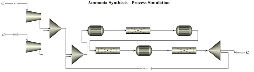
catalyst rapidly reaches a plateau conversion, due to the fact that increasing ammonia concentration decreases the reaction rate, which is not the case for Ru-based catalysts. This may suggest the development of multibed reactors, with intercooling, using the Fe-based catalyst in the first layers and Ru (more expensive) in the last one, only, to achieve the higher conversion unattainable with Fe. Process simulation and optimization of reactor design and operative conditions are currently in progress by our group, implementing the kinetic parameters in Aspen Plus®. The work was planned after a thorough screening of the literature surprisingly revealed a lack in combining kinetic experiments with simulation software. Then a proper simulation of the best industrial technology available using Ru catalyst was carried out (namely the KAAP technology). The reactor is composed of three beds (the first one based on iron while the others based on ruthenium), represented for the simulation as three different plug flow reactors with intermediate cooling (Figure 1).

Figure 1. Flowsheet of a multibed reactor for ammonia synthesis.

Yu et al. tried to implement the kinetic parameters of ammonia synthesis for the evaluation of a coal-based polygeneration process to coproduce synthetic natural gas and ammonia [12]. Unfortunately, the way the kinetic parameters were implemented in the simulation was not detailed, probably for conciseness in the economy of the work which was a complete design and economic evaluation from air and coal to ammonia and electric energy production. Many design variables were investigated, considering the total annual cost. Concerning the reactor, the total annual cost decreased as the system pressure increased, because the enhanced density and thermodynamic driver decreased the required reactor volume and the catalyst loading, overcoming the higher cost of compression.

At the opposite side, Arora and co-workers investigated a small scale ammonia production from biomass [13]. The flowsheet implies the biomass gasification through a dual fluidized bed gasifier configuration for the production of syngas, which is then purified from COx by Pressure Swing

Adsorption (PSA) and methanation. An air separation unit provides pure nitrogen and the ammonia reactor produces the ammonia stream. The Redlich−Kwong Soave, corrected by Boston Mathias (RKS-BM) thermodynamic package was used to model the entire flowsheet. This property package is suitable for processes that involve non-polar and real components, such as gas production, gas processing, and hydrocarbon separation. Gibbs and equilibrium reactors were used to model the ammonia converter. This choice was properly motivated considering that the reaction usually approaches the equilibrium conversion. However, this point should be considered more in detail. The model was validated against some plant data reported in literature.

Ammonia production via integrated biomass gasification was studied by Andersson and Lundgren [14]. The process simulator was used to model energy and material balances of the complete biomass gasification system including the NH3 synthesis. The most important modelling

balance. Also in this case the reactor was simulated using a Gibbs reactor at 180 bar and 440°C, formally using an iron promoted catalyst.

A control structure design for the ammonia synthesis process was carried out by Araujo and Skogestad [15]. The reactor configuration was based on an industrial fixed-bed autothermal reactor. The reaction kinetic was described by the Temkin–Pyzhev expression and the beds were modelled in Aspen Plus® by means of its built-in catalytic plug-flow reactor. The evaluation of the effectiveness of a control structure against disturbance was carried out using the dynamic simulation package.

1.3 – Effect of transport phenomena

Diffusion in porous solids is another key factor to compute, because of the possibly controlling mass transfer during the heterogeneous catalytic process. This point must be taken into account and properly implemented in the simulator software considering where necessary the bulk or Knudsen modes of diffusion in small pores. This problem occurs not only in heterogeneous catalytic process, but also in classical gas-solid reactions. For instance, Mahinpey and co-workers studied the CO2

capture technology using several calcium oxide sorbent materials [16]. The trend of CO2 adsorption

and reaction was simulated by Aspen Plus®, matching the experimental results obtained in parallel experiments. A Plug Flow Reactor was adopted as carbonator reactor, while a Gibbs reactor was chosen for the comparison with the thermodynamic equilibrium conditions. A marked difference between the predictions and the conversion derived from the experimental data was observed and attributed to the grain model used for the calculation of the reaction parameters. The possibility that internal points of the sorbent were never touched by the reactant gas was not taken into proper account by e.g. modelling the concentration profile across the catalyst particle and this led to the discrepancy. The authors suggested that a proper optimization can be done considering these not accessible zones.

1.4 – User defined models

Another approach must be adopted for processes which cannot be simulated. One of the most representative example in literature is the biomass gasification in dual fluidized bed reactor [17]. This technology includes two reactors in series: the gasifier where biomass is converted by steam into syngas (H2 + CO) and a combustion reactor fed with sand and char able to supply thermal energy to

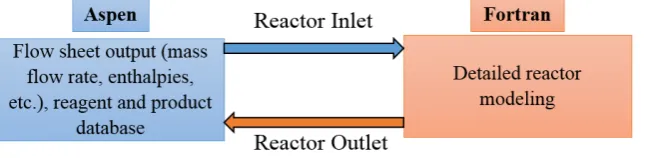
the former. None of the commercial process simulators (Aspen plus, ProII, Hysys, etc.) have predefined models to simulate biomass gasification. Therefore, the kinetic model must be implemented in external files, elaborated with proper software such as Matlab® or powerful scientific programming tools such as Fotran. Abdelouahed et al. exploited the flexibility of Aspen Plus inserting several Fortran blocks, combining complex reactor models and Aspen Plus tools [17]. Reactor modelling can be done by empirical correlations (product yields as a function of temperature), chemical kinetics, or more detailed reactor computations. The output of the flowsheet preceeding the reactor simulated by Aspen Plus® (mass and enthalpy flow rates, temperature, pressure, etc.) is transferred to Fortran modules for the calculation and then transferred back to Aspen (Figure 2). The possibility to implement user defined models makes the difference between the various process simulators.

Figure 2. Conceptual block diagram: coupling Aspen Plus flowsheet with external Fortran modules

2 – Processes following complex kinetic schemes

From the above reported examples, the need of a sound kinetic model to compute the reactants/products evolution under different reaction conditions appears as a must to be fulfilled for reliable previsions. As the complexity of the reactions carried out in the process increases, this becomes one of the key issues to be settled prior to process design. In the following, we will consider the emblematic case of ethanol valorisation into hydrogen or ethylene, as a pathway to the biorefinery exploitation [18–21]. In this view, a biomass-derived raw material is used to provide important chemicals/fuels in a more sustainable way. This idea has to prove sustainable from the industrial and economical points of view, therefore process simulation is a powerful tool for preliminary process design, to evaluate the operating conditions and process layout that may ensure the economical viability of the process.

Process simulation has been carried out to evaluate the performance of a 5 kWelectrical + 5 kWthermal

cogeneration unit starting from bioethanol and converting the reformate by means of fuel cells [22– 25].

2.1 - Simulations of Reforming Processes

Process simulations based on commercial software, firstly developed to meet the needs of the industrial process engineers, thanks to their flexibility are becoming increasingly more popular also as powerful research tools. With these packages, the global heat and material balances of a chemical process can be addressed starting directly from the flow diagram, virtually for every size of the equipment involved and amount of the reactants/products treated, thanks to the extensive collection of pure components properties and thermodynamic correlations available to calculate mixture properties. The main drawback of this approach are essentially: i) the tedious procedures needed to substitute (or to update) such databases with different known data, ii) the relative lack of details in the modeling of the single units of equipment, that can be substituted by custom-made blocks or designed separately with devoted software add-ons, but only spending extra time and efforts to master these tools, and iii) the possibly misleading results (or computational errors) that may arise when too complex chemical systems (azeotropes, immiscible phases, electrolytes) are treated with poorly defined schemes or units hiding nested calculation loops (typically, recirculation lines in the first case and distillation columns or counter-flow heat exchangers in the second).

By contrast, when a robust background is available concerning the reactions, the chemical environment and the basic process layouts, these softwares provide an invaluable tool to size a plant or unit operation, to compare different solutions or to check off-design conditions. So, rather than describing their use as design tools or explaining their fine-tuning when modeling complex, specific situations, this paragraph addresses these softwares as simulators of large process: in this framework, different case histories are reviewed to better show the flexibility and the comprehensive overview achievable.

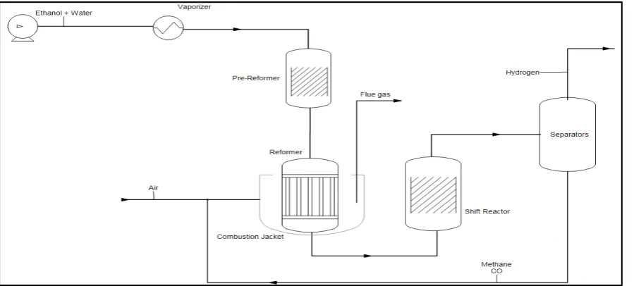
2.1.1 – Hydrogen production by Steam Reforming

as it were fully converted in the same step), 3) from DR, with full conversion of ethanol into CH4 and

CO in a pre-reformer, followed by a separate WGS and MET equilibration stage.

The results are shown schematically in Table 1. The calculations originally performed with PROII [4] have been replaced with similar ones performed in ASPEN Plus® – the same reactor type and SRK thermodynamic model were used. Notice that the calculation scheme shown in Figure 2 of the cited work may not treat rigorously the formation of coke, since two equilibration stages are shown, but only one is modeled via a Gibbs reactor, while nothing is specified about the capability of other PROII reactor classes to mix solid and vapor phases. The differences in these thermodynamic material balances are due to the different setup of the equilibrium reactor blocks in each case, which is the easiest way to account for the catalysts selectivity in a real flow-scheme (where the simultaneous reaction equilibria can be effectively separated in practice).

Table 1: Equilibrium composition (mol/moltot) of a mixture derived from ethanol reforming under the

assumptions specified above; in case 3 Water is fed separately to the second reactor (rather than being treated as inert in the first block).

Molar fractions at 1 atm (feed: H2O:Ethanol = 5:1)

Case 1 Case 2 Case 3

T

(°C) H2 CO/CO2 CH4 coke H2 CO/CO2 CH4 coke H2 CO/CO2 CH4 coke

500 0.30 0.13 0.10 0.00 0.0 0.20 0.00 0.09 0.30 0.13 0.10 0.00

600 0.45 0.50 0.03 0.00 0.52 0.69 0.00 0.00 0.45 0.50 0.03 0.00

700 0.49 0.99 0.00 0.00 0.50 1.02 0.00 0.00 0.49 0.99 0.00 0.00

800 0.48 1.40 0.00 0.00 0.48 1.40 0.00 0.00 0.48 1.40 0.00 0.00

900 0.47 1.82 0.00 0.00 0.47 1.82 0.00 0.00 0.47 1.82 0.00 0.00

1000 0.46 2.25 0.00 0.00 0.46 2.25 0.00 0.00 0.46 2.25 0.00 0.00

Figure 3: Flowsheet for ethanol steam reforming without (top) or with (bottom) a separate stage for the two-step conversion of methane.

With these configurations and the typical operating condition specified below, the overall material balances obtained are as follows (Table 2, [4]). These results are obtained on the basis of the thermodynamic “atom equilibrium”, only, and are therefore useful to find the maximum hydrogen yield or to represent reactors with an excess catalyst hold-up.

Table 2: Principal data from [4]. (*) This datum is referred to the overall flowsheet input.

Case 1 Case 2

Reformer inlet T (°C) 800 650

Reformer outlet T (°C) 850 920

Pre-reformer outlet T (°C) - 370

Separator T (°C) 30 – 35 30 – 35

Ethanol feed (kmol/h) 854 914

Water to Ethanol ratio (mol/mol) 5 5 (*)

Hydrogen to Ethanol yield (mol/mol) 5.2 4.9

ESR grants the highest hydrogen output, but requires also the highest energy input to sustain the reaction. While different strategies are possible to burn directly or indirectly an excess of ethanol (stemming from the basic scheme of Figure 3), another option is to add oxygen to the reactants mixture (this is the so-called Autothermal Reforming, ATR, or Partial Oxidation, POX, strategy, depending on the presence or not of water).

The methodology proposed by the cited authors, however, do not foresee to find the Oxygen stoichiometric ratio which yields ΔrH = 0 (ATR), but to optimize the oxygen amount so to keep a

hydrogen output as high as possible.

Figures 4: Hydrogen yield (mol / mol of ethanol fed) at equilibrium calculated under the specified conditions. O/E = Oxygen/Ethanol molar ratio.

Starting from these findings, Khila et al. [7] extended the analysis giving up the solid carbon species representing the catalyst coking (which is indeed minimised for Steam-to-Ethanol ratios higher than 4 and reforming temperatures above 500 °C, but developing full process flow diagrams with separated WGS and methanation sections for the three options (pure SR, POX and ATR) and analysing the exergy inputs and outputs (see the cited reference for the details of this thermodynamic potential). Their results are synthetically reported in Table 3.

Table 3: Selection of data from ref. [7].

Exergy input (kJ/mol H2) 407.7 H2yield (mol/mol ethanol) 3.42

Exergy output (kJ/mol H2) 295.9 H2O emission (kg/kg H2) 14 Electricity input (kJ/kg H2) 776.6 CO2 emission (kg/kg H2) 12 Ethanol feed (kg/kg H2) 6.73 CO emission (kg/kg H2) 0.00 Water feed (kg/kg H2) 15.8 CH4 emission (kg/kg H2) 0.032

Besides the value of hydrogen as chemical, its preferred use is perhaps the electric power obtained from the Fuel Cell (FC) systems. The coupling of a reforming plus a FC block allows then to simulate the full “Ethanol-to-electricity” process.

Focusing the attention on the general balances, several works are reviewed which treat essentially the cell as an equilibrium reactor: the hydrogen fed is related to the available power (or voltage / current) via semi-empirical correlations that subtract the expectedly wasted energy, or, equivalently, the potential drop and parasite currents [21,26–28].

Starting from the SR reactions, an integrated analysis of the cell power and heat needs has been performed in [9] using HYSIS® and the flowsheet outlined below (Figure 5), with the main findings are reported in Table 4. The details of the heat analysis and its implementation with very specific HYSIS® tools is here omitted and can be found in the cited work. The 1 kW FC is modeled correcting the Faraday relation for ΔErev with a known relation for the potential drops, while the reformer yields

the thermodynamic equilibrium fractions.

1 1.5 2 2.5 3 3.5 4

0 2 4 6 8 10

Hydrogen Yield

(mol/mol EtOH)

Water/Ethanol (mol/mol)

H2Yield from ATR @ 500 °C, 1 atm

Figure 5: overall PFD for the ethanol reforming as described in [9]: the pumps are for water (above) to the reformer, fed with fresh water and condensate from the reacted mixture and from the cell, and ethanol (below) to the reformer (after mixing with water) and directly to the burner. Air to the burner, to the byproducts oxidizer (“PrOx”) and to the cell is provided by the compressors in the lower middle of the scheme. Notice the special multiple-currents heat exchanger-type block (“LNG”), which is more properly a nested subroutine capable of solving a basic pinch analysis (limited, in this case, to a 20 temperature intervals discretisation) of all the cold and hot streams routed through the block. The heat released by the fuel cell is added to the balance of the network via a closed service loop, since the LNG block cannot discharge directly a heat stream on the CU; a HU is not present because the more demanding stream (the already pre-heated reformer feed) is connected to the burner via another heat stream external to the PA block. The image is reproduced by kind permission of Elsevier.

Table 4: Selection of data from ref. [9]; the maximum fraction of methane in every stream is always

lower than 2.5%.

Material Balances

Stream 4 5 7 9 12 14 28

T (°C) 709 709 539 237 406 80 80

P (atm) 3 3 3 3 3 3 3

Flow (kmol/h) 0.0367 0.0628 0.0628 0.0628 0.0658 0.0636 0.1749

Fractions

Ethanol (mol/mol) 0.20 0.00 0.00 0.00 0.00 0.00 0.00 Water (mol/mol) 0.80 0.28 0.24 0.17 0.18 0.15 0.15 Hydrogen (mol/mol) 0.00 0.49 0.52 0.59 0.55 0.57 0.04 CO/CO2 (mol/mol) 0.00 1.17 0.58 0.03 0.00 0.00 0.00 O2 (mol/mol) 0.00 0.00 0.00 0.00 0.00 0.00 0.08

Energy Balances

Cold Streams Cold Utility Hot Streams Reformer Fuel Cell Lower T (°C) 25 – 142 20 80 – 810 709 55 Higher T (°C) 126 – 709 25 406 – 1035 709 65

A conceptually equivalent simulation has been performed by Jaggi et al. [8] with Aspen Plus®, but outlying manually the heat-exchange network rather than resorting to a built-in software feature. Both the reformer and the FC are modeled based on a known stoichiometry (SR plus WGS and MR for the reactor, hydrogen combustion for the cell with assumed values for the electric and entropic powers in which the enthalpy difference is split). Focusing on the balance between the FC output and the thermal energy recovered by the residual methane and CO burning, these authors define the overall system efficiency as the electric power divided by the enthalpy content of the ethanol fed. Their esteems are reported in Table 5.

Table 5: Data from ref. [8] for a FC with the following characteristics: power = 5 kW; nominal stack

voltage = 24 V; nominal cell voltage = 0.55 V; cells in stack = 88; current = 208 A; current density = 0.5 A/cm2_{; cell area = 406 cm}2_.

Parameter FC T = 200 °C FC T = 180 °C FC T = 160 °C

Output ΔV/ desired ΔV (V/V) 0.55 0.55 0.55

Current density (A/cm2_{) 0.5 0.37 0.2}

Current drawn (A) 208 153 83.2

Electric Power (kW) 5 3.7 1.99

Overall efficiency 0.45 0.33 0.18

One can notice that both these configurations can be considered as “autothermal reforming” ones, from a general point of view, since a co-feed of oxygen is actually injected in the burners, giving overall enthalpy balances more favorable than those of the pure SR without necessarily add fresh fuels to this section – the situation, however, retains a practical difference since the heat exchange network is perforce different from the true auto-sustained configuration of a non-endothermic reaction.

These results define then the thermodynamic boundaries of the ethanol reforming process as calculated with the state of the art process simulators.

Moving further, a “native” ATR process has been calculated by Aicher et al. [10] in a study that combines steady-state simulation, experimental data and dynamic recording of several process variables (the used software is Chemcad). Despite the lab-scale of the study, it is interesting to notice that the used plug-flow reactors can be actually simulated by equilibrium/stoichiometry modules in the proper conditions and catalysts hold-ups. The hydrogen output is quite high (Table 6) and is obtained with a minimal heat-exchange configuration (just the Product-to-Feed auto-exchange is present, plus the combustion), though the authors do not give the full material and heat balances to discriminate between the “in-reactor” energy saving and the heat released in the other combustions.

Table 6: Data from ref. [10] for a process configuration involving a reformer, two WGS stages and one

methane post-processor in series (MR). Feeding Water / Ethanol = 5 mol/mol; feeding Oxygen / Ethanol = 0.9 mol/mol; reformer inlet = 390 °C.

Unit output T (°C) measured

H2 (Vol/Vol %) CO/CO2 (Vol/Vol %) CH4 (Vol/Vol %)

measured simulated measured simulated measured simulated

ATR reactor 745 37.6 38.8 2.00 1.71 0.13 0.01

WGS stage 1 400 41.5 42.9 19.8 11.5 0.13 0.01

WGS stage 2 290 41.9 43.5 93.18 41 0.13 0.01

MR reactor 220 40.8 42.6 - - 0.67 0.52

with the same tools as in [9]), while the “slow”, time dependent, sections that link the equilibrium ones are calculated with Matlab. All the reactors are treated as plug-flow ones, with full Arrhenius expansions of the reaction rates, and also the mass balances of the FC are treated as transient.

The interested reader may find every computational detail in the given reference. Here we point out that the whole analysis is meant to control the H2 flow to the FC, and the foreseen control system

handle very well a variation in the electric power requirement, while it cannot avoid some spurious peak in the hydrogen yield in front a variation of ethanol purity.

The same equipe refined further the above described control system [6], reassessing its validity and comparing the effectiveness of different control strategies (based on different process parameters on which to base the system response) when the integrated reformer/FC system is to be used for automotive purposes.

We complete the excursus considering other two simulations. The first [29] compares the SR and ATR processes. The calculations were done with ASPEN Plus®, with two different heat-integration configurations for both cases, of two different feedstocks, ethanol and bio-diesel (represented mainly as maleic-oleate). The gas flow composition at the FC inlet in the selected operative conditions are lumped in Table 7 for an easier comparison.

Table 7: Data extracted from ref. [29]. SR performed with reactor outlet at T=800 °C and feeding

Water/Ethanol = 6 mol/mol; ATR performed with Oxygen/Ethanol = 0.35 mol/mol and Water/Ethanol = 4 mol/mol. Methane was always absent.

Steam Reforming Fractions (Vol/Vol %)

ATR Fractions (Vol/Vol %)

Species Ethanol Biodiesel Ethanol Biodiesel

H2 54.1 56.8 29.6 30.5

H2O 27.7 22.9 24.3 19.6

CO/CO2 0.022 0.025 0.013 0.018

N2 - - 30.3 32.5

The second case [30], performed with HYSIS®, compares the hydrogen yield obtained from a conventional Ethanol Steam Reformer to the one coming from an electro-chemical reformer (Table 8). Since the data on the operative performance of the two different reactors are found elsewhere (see references addressed in the cited work), the interest of this simulation lies mainly in the fact that the electrical process required a simpler configuration, since the heat-exchange network and the pre-heating were not needed.

Table 8: Data extracted from ref. [30].

Steam Reforming Electrical Reforming

Hydrogen Yield (kg/kg EtOH) 0.03 0.044 Overall Energy Input (kWh/ kg H2) 33 28

From the above reported examples, the need to properly predict the behaviour of the different reactors underlines the requirement of complete and reliable kinetic models as the basis for this simulation activity. This point will be addressed in the following sections.

2.2 - Kinetic and Theoretical Analysis of Ethanol reforming

the reforming products mixture with the one expected at thermodynamic equilibrium; 3) the rationalisation of these data in terms of a chosen mechanism.

The first step involves mainly a catalyst synthesis, characterisation and activity testing: statistical procedures help indeed in the eventual interpretation of data [25], but at this stage the most important goal is the correlation of a products yield to the relevant catalyst features, or the comparison between different catalysts: as an example of this kind of analysis, see the various species yields on different materials as tested in [31].

At the second step, the catalyst selectivity towards a whole reaction path rather than towards a product becomes clearer. In fact, since equilibrium conditions depend on the temperature (most of the test reactors works with negligible pressure drops), when the full conversion of the precursor is achieved then the possible byproducts reveal that a certain path is kinetically forbidden (or enhanced), and if the ratios of H2O, CO, CO2, H2 and CH4 differ from the thermodynamically expected ones then

even equilibrating reactions are kinetically delayed. Therefore, the study of reforming mixtures as a function of the reaction temperature can show if a material is always active towards any reaction path until the ultimate equilibrium or, on the other side, if the activation barriers between each reaction are appreciably different (for this kind of analysis, see for example the above cited papers and [32– 34]).

The third step can be performed essentially in two ways: i) a mechanism is postulated according to the intermediates, then the relative reaction rates are extrapolated evaluating the amount of products as a function of the contact time (which, at this stage, becomes the most important parameter), then the variation of the temperature allows the extrapolation of the activation energies; ii) the interaction between reactants and catalyst is studied a priori relying only on the quantum mechanical models of the interacting atoms: virtually any possible bond break and formation (or a wide selection of them) is tested and the corresponding elementary reaction rate is quantified (via the Eyring model) until all the steps from reactants to products are linked.

2.2.1 - ESR: conversion rates and steady states

As shown by equilibrium calculations (for example [35,36], for two different methodologies) a sufficient loading of a catalyst with the correct selectivity towards the reforming can eliminate any byproduct (except methane) when working at the proper temperature.

In this context, the simplest kinetic model that can be formulated on the stoichiometric ground is as follows:

+

→

+

+ 2

+

⇌

+ 3

+

⇌

+

In order to quantify just the conversion rate of ethanol, mass-transfer steps (i.e. how the species diffuse through the material pores and within the gaseous stream) are typically not relevant for the reaction. The equilibrium reactions, in turn, do not affect ethanol conversion if this is truly not-reversible (tests performed in plug-flow reactors actually divide ethanol conversion and equilibration also spatially). If, moreover, the water to ethanol ratio is sufficiently high and the reactants are diluted in an excess of inert carrier, then the model can be reduced to a pseudo-homogenous first-order one:

= −

with

=

exp (− )

If the water to ethanol ratio in the mixture is not high enough and the first-order simplification has to be dropped, the next step is to resort to an empirical general formulation based on kinetic pseudo-orders:

= −

This kind of analysis is used in [37–39], where catalysts of Ru/Al2O3, Ni/MgO/Al2O and Ni/Al2O3

yielded the following kinetic parameters (Table 9). Notice very small values of the activation energy, which may indicate the presence of diffusional limitations or of highly correlated parameters.

Table 9: Data as from Table 2 of ref. [37], equation 6 of ref. [38] and Table 4 of ref. [39]. The values for

and from ref [37] (not reported in the same form, but as calculated constants at different temperatures) have been fitted with Excel™ REGRLIN (r2 _{= 0.9446), while the power-law model of} ref. [9] was originally presented in terms of molar flowrates rather than partial pressures.

a b

Ref. [37] (Ru/alumina)

55881 (cm3 _gcat-1 _h-1_{) 42 (kJ/mol) 1 0}

Ref. [38] (Ni/MgO/Al2O)

439 (mol min-1 _gcat-1 _atm -3.42₎

23 (kJ/mol) 0.711 2.71

Ref. [39] (Ni/alumina)

0.031 mol gcat-1 _s-1 _{4.41 (kJ/mol) 0.43 0}

Moving further and considering that the outcome of this conversion is a mixture of four species, the amounts of CH4, CO, CO2 and H2 can provide an idea of the kinetic importance of the equilibria

with respect to the conversion. For example, the study performed in [40] reported the following outcome (Table 10) on the state of methanation reaction over a Rh catalyst supported on Ceria-Zirconia.

Table 10: Data extracted from Table 5 of ref. [40].

Temperature (°C) 500 550 600

Yield (mol/mol Ethanol)

measured equilibrium measured equilibrium measured equilibrium

H2O 4.00 2.99 4.00 2.68 2.36 2.41

H2 1.56 2.15 1.85 2.96 3.63 3.78

CO/CO2 0.64 0.25 0.61 0.32 0.48 0.62

CH4 0.21 0.93 0.28 0.68 0.50 0.39

C2H4 0.025 0.000 0.015 0.000 0.000 0.000

In the same work, the activity of the catalyst towards the WGS reaction was tested, showing values nearer to the equilibrium ones, but only in certain temperature ranges and with a dependency on the feed composition. Therefore, the authors concluded that, even if no intermediate conversion products ‘survive’, their production/conversion rates are comparable with the rates of the ‘lumped’ ethanol conversion and of the equilibration steps, and that the mechanism leading to methane (and from it to CO and CO2) depends on the catalyst.

2.2.2 - ESR: from stoichiometry to mechanism

break) and lumped methanation and WGS reactions into one stoichiometry but allowing for two different paths:

1)

+ ∗ ⇄

2)

+ ∗ ⇄

₊

3)

+

⇄

+ 3

+ ∗

4)

+ 2

→

+ 3

+ ∗

Barring the detail, and noticing that this work does not account for CO in the mixture or on the catalyst (Ni/Al2O3), we point out that even this simple analysis yielded comparable activation

energies and mean square errors (MSE, we mean calculated concentrations versus measured ones, for the best extrapolated values of the kinetic parameters) when the RDS was considered the 2nd _or

the 3rd_{, confirming on a purely kinetic ground that the methanation and WGS reactions may be not}

faster than the C-C break and sensitive to the mechanism being actually followed.

Table 11: Data taken from Table 4 of ref. [39], prefactors of the kinetic constants are not reported, since

the different tested mechanism lead to a difference in the reaction orders and then in the measuring units. The MSE is reported by the authors as the absolute value of the deviation between predicted and observed conversion rates, normalised to the observed rate.

RDS Ea (J/mol) MSE

2 4430 6.0 %

3 3550 10.6 %

By only considering qualitative data obtained below 100% conversion it is possible, though, to discriminate another RDS even prior to C-C break, for example the formation of acetaldehyde as the main path for oxidative ethanol reforming (for example: [41,42] among others), even when this chemical is not recognised in the product mixture thanks to the catalyst loading or other reaction conditions that favor its fast conversion into methane. A simple, yet straightforward, step in this direction is the work by Wang et al. [43], who maintained the basic stoichiometry already described with another sets of 4 elementary steps:

1)

₊

_{+ ∗ → 2}

_{+ 4}

_{+ ∗ + ∗ + ∗}

2)

_{+ ∗ + ∗ →}

₊

_{+ ∗ + ∗}

3)

+ ∗ →

+

+ ∗ + ∗

4)

+

+ ∗ ⇆

+

+ ∗ + ∗

Contextually, the same authors showed (thanks to a collection of data taken on a Ir/CeO2 catalyst

addressed at least in an heuristic way. the interested reader can further investigate this point with the help of the data contained in Figures 4 to 7 of the above mentioned work and of the synthetic review of several power-law models (Table 2, ibidem). Here we just notice that, despite the simplicity of the proposed mechanism -- basically, a stoichiometry for the path: ethanol  acetaldehyde 

methane ,-- the addition of a further kinetically relevant stage actually improves the description of the reforming process, and the choice to separate the adsorbed species into two different adsorption sites is consistent with the recognised importance of the support material beside the active metal. At a glance, the main findings of this work are reported in Table 12.

Table 12: Data taken from ref. [43] (see also references therein) for the rates of the above RDS and for

the adsorption equilibria of the relevant species on the catalyst: the constants are calculated at 818 K and the tolerances at the 95% confidence level.

RDS K (mol kgcat-1 _s -1₎

Ea (kJ/mol) Species K (kPa-1_{) ∆H (kJ/mol)}

1 11 ± 1 85 ± 14 ethanol 25 n.a.

2 9 ± 0,01 32 ± 15 water 3 × 10-4 _-55

3 23 ± 5 66 ± 29 CO2 2 × 10-3 -67

4 20 109 ± 19 CO 1 -80

H2 0,01 -110

In parallel, Mas and coworkers [44] developed the reforming mechanism considering the production of methane, giving less importance to the aldehyde as a kinetically relevant intermediate, but helping to establish the methanation reaction as a RDS itself (rather than a fast equilibrium stage), accounting for the different behavior of this species on different catalysts.

The same authors substantially refined the first proposed kinetic model in a later work [45], based on an extensive data collection obtained by tests on a catalysts of Ni/alumina and Ni(II)/Al(III), taking advantage of the mechanism selection already worked out by Graschinsky et al. [46] (data from a Rh/magnesia/alumina catalyst) and of a similar work by Sahoo et al. [47] to explain their own data (Co/alumina). While these papers share the same core of RDS, the latter authors adopt an abridged stoichiometry where the methanation is not treated explicitly, as it were just the ‘equilibration link’ between “dry reforming” and a full “steam reforming”. In any case, acetaldehyde is considered as the key intermediate, even if rapidly converted before its possible desorption, via a sequence of steps such as:

1)

_{+ 2 ∗ ⇄}

_{+ 2}

2)

_{+ ∗ ⇄}

₊

3)

+ 2

_⇄

₊

₊

4)

+

_→

₊

5)

+

_⇄

₊

in conditions where byproducts and coking can be neglected. A brief selection of values is outlined in Table 13 for the following common stoichiometry:

1)

+

→ 2

+

+

,

2)

→

+

+

,

3)

+ 3

→ 6

+ 2

4)

+

⇄

+

,

Table 13: Data from ref. [44–47]. (*) this reaction is found written in the inverse sense; (**) the original

paper reports likely mistyped units: the values are useful only for a comparison of the relative values.

Ref: [44] [45] [46] [47]

cat Ni/alumina Ni(II)/Al(III) Rh/ MgAl2O4/

Al2O3

Co/Al2O3

k1 - 3.06 × 10-7 _{(mol mgcat}-1 _min-1_{) - -}

k2 - 1.13 × 10-7 _{(mol mgcat}-1 _min-1_{) - 4.46 × 10}+19 _(m2 _mol-1 _s-1_{) (**)}

k3 - - - 1.16 × 10+20 _(m2 _mol-1 _s-1_{) (**)}

k4 - 9.12 × 10-4 _{(mol mgcat}-1 _min-1₎

(*)

- 4.64 × 10+16 _(m2 _mol-1 _s-1_{) (**)}

Ea1 235.06 (kJ/mol)

195.5 (kJ/mol) 418 (kJ/mol) -

Ea2 278.74 (kJ/mol)

122.9 (kJ/mol) 85.9 (kJ/mol) 71.3 (kJ/mol)

Ea3 - - - 82.7 (kJ/mol)

Ea4 - 166.3 (kJ/mol) (*) 107 (kJ/mol) 43.6 (kJ/mol)

2.2.3 - Other Reforming Models

All the above cited models, though developing the reaction pattern yielding all the equilibrium reforming products, rely on data collected with reactors that can be treated by the ideal isothermal, isobaric PLUG-FLOW model, with neither any axial back-diffusion of the chemicals nor any mass transfer limitations. The correct modeling of these latter kinetics requires the implementation of PDE systems for every mass transport mechanism and possible heat transfers, if the foreseen system requires it. Without going into the details of this wider research field, we briefly account for at least three interesting aspects: i) the intrinsic mass and heat transfer limitations of wall-coated microchannel reactors [48–50]; ii) the time on stream-dependent kinetics due to the (relatively) slow and selective adsorption/release of a species [51,52]; iii) the former phenomenon described in non-ideal reactors characterised by temperature as well as pressure gradients [53,54].

2.2.4 - ESR: from chemical bonds to Hydrogen

Increasingly complex reaction mechanisms and thus kinetic models may result in very complex kinetic testing. This is needed to provide sufficient experimental data to account for increasing number of parameters to be fitted. Nevertheless, complex kinetic models may end in strongly correlated kinetic parameters, which at the end may loose reliability.

Reverting the perspective, and the possibility to look at the reaction mechanism at atomic level

and just ab initio (without any prior selection of intermediates to be found), is nowadays possible thanks to the increased availability and reliability of computational algorithms based on a first-principle quantum mechanic approach. All the works reviewed here resort to a specific electronic structure method called Density Functional Theory to estimate the interaction energy between atoms while taking into account the composition of the catalytic materials and the arrangements of the atoms in the solid. In principle, this approach may support kinetic modelling, providing independent kinetic or thermodynamic parameters, thereby limiting the number of parameters to be estimated by regression of kinetic data, hence the correlation between parameters.

Considering an Ethanol molecule interacting with a solid, a straightforward pre-selection of the relevant bond-ruptures allows to concentrate on the C atom linked to the Oxygen, giving four possible initial routes for the decomposition (Figure 6):

Figure 6: The four bond breaking options relative to the C atom linked to the oxygen. It represents

the starting point in many analyses on ethanol degradation. The top two paths are considered distinct.

The route to each possible product across the potential energy surface is then explored to find the lowest-energy barrier to overcome, so that the activation energy and heat of reaction can be determined for each elementary step. With this approach, Wang et al. [57] compared the relative energy barriers for the above mentioned initial paths on a whole set of noble metals. The analysis was also repeated for these dissociation paths to take place after the initial dehydrogenation EtOH  EtO

-. Without reporting all the data, one of the more probable reaction mechanism is shown below, as asserted for Rh and Ni (1,1,1) crystalline plane (Table 14 and Figure 7).

Table 14: Data from ref. [57], showing the energetic barriers and heats of reaction (eV) of the indicated

elementary steps, selected as the favorite ones.

Step Rh Ni

1) ∗ → ∗ ∗ + ∗ 0.52 / 0.45 1.46 / 0.51

2) ∗ ∗ → ∗ ∗ + ∗ + ∗ 0.42 / -0.69 0.14 / -0.73

3) ∗ ∗ + ∗ + ∗ → 2 ∗ + ∗ + ∗ 0.99 / 0.82 1.04 / 1.02

4) ∗ → ∗ ∗ + ∗ 0.55 / 0.52 1.57 / 1.15

5) ∗ → ∗ ∗ + ∗ + ∗ 0.05 / -1.10 0.10 / -1.33

6) ∗ ∗ + ∗ + ∗ → 2 ∗ + ∗ + ∗ 0.97 / 0.84 1.05 / 1.01

CH3–CH–OH + H CH3–CH–OH + H

↖ ↗

CH3 – CH2 – OH

↙ ↘

Figure 7: Graphic representation of the elementary reaction steps relative to Table 14; the initial adsorbate is conventionally placed at the ‘zero’ energy level.

In this paper, the interested reader also finds a correlation between the activation energies of these transitions and an energetic parameter representative of these d-transition metals, what is known as d-band model [58].

A similar analysis was performed later by Sutton and Vlachos [59], who tried to correlate the preferred reaction paths on six transition metals to their ethanol-binding ability, rather than on more general lattice properties: the authors established a link between the M-O binding energy and several critical bond-ruptures (e.g. C-C, C-O), while a comparison between the modeled metals can be appreciated at a glance in Figure 8:

Figure 8: Sketched preferential paths on six noble metals as outlined in ref. [59].

The same authors focused later on platinum [60], performing an extensive analysis of all the possible bond-breakings from ethanol down to carbon monoxide together with the reversible de-hydrogenations linking methane to the CHx groups. This comprehensive study is complemented by

-0.6 -0.2 0.2 0.6 1 1.4 1.8

1 2 3 4 5 6 7

dE (eV)

Reaction Step

Calculated energetic profile of Ethanol degradation

the fit of a set of conversion data, obtained adjusting just a scale-normalization factor. Importantly, this first-principle analysis confirms the kinetic relevance of the H-abstraction steps that lead to acetaldehyde formation, postponing the C-C breaking stage, and the eventual re-equilibration of the fragments as precursors of CO, CO2 and methane.

Figure 9: Synthetic scheme of the reforming mechanism, adapted from ref. [60].

A similarly comprehensive mechanism on Platinum was developed by Koehle et al. [61] for ethanol partial oxidation, where the total amount of reaction steps (50, each one considered in principle as reversible) was treated with a less aprioristic approach. The activation energy of every bond-break was estimated with a semi-empirical model, the so-called UBI-QEP, that relies on the interpolation of the calculated (or measured) binding energies of the intermediates with two parameters, catalyst coverage and temperature, that are in turn eventually used to extrapolate the activation energies separating an intermediate from to the other.

Though less rigorous from the theoretical point of view, this work also presents the fit of another set of reforming data, obtained by adjusting less than 10 (out of possible 100) of the already calculated pre-exponential factors. Interestingly, the adjusted reaction steps were chosen via a statistical sensitivity analysis, which points out methane formation and CO oxidation as crucial for the product distribution in the mixture.

2.3 - Ethanol to Ethylene

2.3.1 - Ethanol to Ethylene: direct dehydration

The conversion of ethanol to ethylene is catalysed by acidic catalyst functions, often attributed to Lewis type sites. It may be the desired reaction for the production of this building block from a renewable source, or it may represent a reaction path parallel to the oxidative one, leading to acetaldehyde and then to carbon-carbon scission and conversion into hydrogen/syngas [62]. In this sense, it is an undesired path because it lowers the H2 yield, and it is connected with catalyst

deactivation by coking. In any case, its kinetics should be detailed in order to perform process simulation or to cope with selectivity/durability issues. Also for this application, first principle methods may help addressing possibly complex reaction pathways.

selectivity ‘a posteriori’, analysing those points whence expected byproducts or alternative routes stem. Following this approach, a very straightforward yet indicative DFT calculation of the dehydration in differently doped Zeolites was performed in [63] (Table 15).

Table 15: Data from ref. 7 for the reactions: (a) EtOH*  [TS‡] and (b) EtOH  C2H4 + H2O.

H–ZSM–5 Cu–ZSM–5 Ag–ZSM–5 Au–ZSM–5

∆ ‡( ) _{kcal/mol 43.86 52.75 40.1 36.29}

∆ ( ) _{kcal/mol 4.76 4.76 4.76 4.76}

The choice of just one reaction path for every catalyst with the C-O bond progressively loosing may be somehow simplified, but it establishes a direct link between theoretical calculations and the well-known empiric concept of “functional group”, still applicable with catalysts and conditions, which yield a 100% selectivity.

Moving a step further, Kim et al. [64] extended the a-priori study of the dehydration in two directions, even if focusing on the H-ZSM-5, only: a comparison between two different mechanisms and a benchmark of different computational strategies. We report here a synopsis of the main findings (Table 16 and Figure 10); the reader can check out the computational and mechanicistic details in the cited reference with its supporting material.

Figure 10: Schemes of the mechanisms studied in for ethanol dehydration on a

zeolite catalyst

[64].

Table 16: Data from ref. [64]. The reference zero-energy is the lowest of the binding energies of

adsorbed ethanol on one of the 4 O-atoms available at each site: since any of the two mechanisms can then yield different energetic profiles (according to the different O atoms possibly involved), the reported values are the averages, for a given TS, over all these possibilities.

Computational method 1 Computational method 2

Intermediate ∆E ∆G ∆E ∆G

A similar study was performed by Maihom et al. [65] for an Iron-doped zeolite (Fe–ZSM–5), analysing the steric and energetic features of two mechanisms (Figure 11), a step-wise (where ethanol interacts with one catalyst atom at a time) and a concerted one (where ethanol interact simultaneously with two catalyst atoms).

Figure 11: Schematic summary of the mechanisms proposed in ref. [65].

Qualitatively, it is interesting to note that the mechanism with the higher energetic barriers is not completely excluded, because it shows the lowest barrier for the initial step – moreover, the ‘choice’ between the two paths depends strongly on the orientation of the alcohol inside the adsorption site.

2.3.1 - Ethanol to Ethylene: parallel paths

Though only incidentally, in the above works the possibility that–H atom transfer takes place via a bimolecular reaction with a nearby ethanol molecule rather than with the catalyst is also addressed, instrumental to ethylene formation. This phenomenon is related to a possible byproduct of the reaction, i.e. the di-ethyl ether (DEE).

Christiansen et al. [66] studied theoretically the reaction of ethanol on γ-alumina, assigning ethylene formation to an unimolecular mechanism (either step-wise or direct), and further explaining how a bimolecular mechanism may also yield ethylene, but will more likely turn ethanol into DEE (Table 17). Moreover, comparing the reaction rates predicted by the model with a set of experimental data, these authors were able to discard less relevant reaction paths still fitting the observations with a minor adjusting of the already calculated parameters. The inferred mechanism and basic stoichiometry are sketched in Figure 12.

Table 17: Most important elementary steps of the mechanism explained in [66], with the free energies of the intermediates compared to gas-phase values (all numbers in kcal/mol, for T=488 K). Superscripts ‘Al’ and ‘O’ denotes catalysts active atoms.

Elementary step Δ Δ ‡

(calculation)

Δ ‡_(adjusted)

+ ⇄ + -12 2 2

+

⇄ + -7 28 24

+

⇄ + +

-16 21 17

+ ⇄ + + -16 25 29

⇄ + -4 58 58

Figure 12: Paths for ethanol conversion to DEE and ethylene [66].

1)

+ ⇌

2)

+ ⇌

3)

+ ⇌

+

4)

+ ⇌

+

5)

+ ⟶

+

+

6)

+

⟶

+

An extended representation of the process was outlined by Alexopoulos et al. [67] for the already mentioned zeolite HZSM5: the parallel ethylene / DEE figure is modified into a three-fold macro-scheme (Figure 13), where the paths A, B and C represent in turn a succession of simultaneous and competing elementary steps.

These authors consider again only the catalyst oxygen atoms as directly involved in the bond activation process, however their extended reaction network was able to reproduce a set of contextually collected data without further adjusting the parameters. The relative weight of the possibly competing routes leading to each experimentally observed product was evaluated by a statistical analysis of the calculated reaction rates. Moreover, the authors considered ethanol absorption more important than water in determining the selectivity and the change of mechanism during the conversion. For a more specific comparison, we report the results obtained for the most probable routes to ethylene [A/1-2-3-4-5] and DEE [B/1-6-7-8-9] as extracted from the above cited paper [67] (Table 18).

Table 18: Data from ref. [67]: any step being reversible, equilibrium constants are always calculated

via the Eyring model, while Ea and A refer to the Arrhenius formulation, and are defined only for rate determining steps (RDS). These, in turn, are selected by the authors on the basis of a statistical screening of the Keq values over a larger range of temperatures and catalyst coverage. Single H* and O* denote active atoms present on the alumina after moisture adsorption. A is given in (s-1_{) or (10}-2 kPa-1 _s-1_{) for RDS or adsorptions, while Keq is reported in: (10}-2 _kPa-1_{), (10}2 _{kPa) or dimensionless for} adsorption, desorption or reactions at the surface, respectively.

Elementary step Ea

(kJ/mol)

A (*) Keq(**) @ 500 K

Kinetic relevance

1) + 2 ∗ ⇄ ∗ ∗ - - 1.1 × 104 _equilibrium

2) ∗ ∗⇆ ∗ + ∗ - - 8.0 × 10-2 _equilibrium

3) ∗ + ∗+ ∗

⇄ ∗₊

118 4.0 × 1013 _{3.8 × 10}-1 _RDS

4) ∗ ⇄ ∗+ ∗+ ∗ 106 9.4 × 1012 _{3.5 × 10}-2 _RDS

5) ∗⇆ - - 1.4 equilibrium

6) ∗ ∗+ ⇄ ( ∗) −

− ∗

- - 7.6 × 101 _equilibrium

7) ( ∗) − − ∗

⇄ ∗

+ ∗

- - 4.5 × 10-4 _equilibrium

8) ∗ + ∗⇄ − ∗−

+ ∗

92 3.5 × 1012 _{7.2 × 10}4 _RDS

9) − ∗− ⇄ + ∗ - - 1.3 × 10-6 _equilibrium

Figure 14: Reaction schemes outlined in references [62] (left) and [68] (right).

Afterwards DeWilde et al. [62] re-addressed from an experimental point of view the original discrimination between ethanol dehydration and dehydrogenation, applying also techniques of isotopic labeling and co-feeding pyridine alongside ethanol and water. The main finding of this work, besides the proposed re-hydrogenation of ethylene to ethane, can be summarised as follows: i) at T>600 K water is effectively desorbed from the catalyst, making the conversion rates again insensitive to its partial pressure, ii) unimolecular reaction paths are kinetically determined by C-H breaks, while the DEE production is regulated by –O bonds cleavage; iii) pyridine decreases the yield of both ethylene and acetaldehyde, confirming that the required –H abstraction step takes place on acidic sites.

This suggests that other factors, besides catalyst acidity, can be relevant in the possible yield of acetaldehyde also in ethanol dehydration reactions. Nevertheless, the ethylene production rate constant was given a kinetic pre-factor about 80 times larger than that of acetaldehyde [62], and this poses a substantial quantitative difference between these catalysts and the actually basic ones (e.g.

Lanthana or Ceria – see for example the data on ethylene/acetaldehyde selectivity reported by [34]. The interplay between the ethylene/DEE reaction paths was lately reassessed by Knaeble and Iglesia [69], either experimentally (on acidic mixed metal catalyst supported on silica) and with a combined a-priori (DFT based) heuristic calculation (Langmuir-Hinshelwood model with fitted parameters).

Figure 15: Reaction paths as traced in [69], built upon the catalyst regeneration cycle.

A complete DFT analysis of the relative transition states was contextually performed, and an “energetic profile” of the reaction was obtained as reproduced in Figure 16. The kinetic constants determined for the elementary steps were then statistically screened via a sensitivity analysis similar to the one mentioned above (i.e. examining the dependence of a certain yield on a small variation of the kinetic factors), since this considerably reduces the number of parameters actually needed for the model to account for the observed data.

Figure 16: Gibbs Free Energy profile from ref. [69], relative to mechanism reported in their Figure 7.

After the selected kinetic parameters were adjusted to reproduce the observed data, they were compared with their bare values (i.e. those computed at the DFT level), and the same trends were found as a function of the energy required to exchange one H+ _{unit between reactants and catalyst.}

As a result, the authors of the above work concluded that the bimolecular or concerted C-H and C-O breakings dominate for both ethylene and DEE production.

Up to this point, the selectivity issue seems to concern a minor yield of DEE, while it must be remembered that acidic catalysts do promote the polymerisation of ethylene into aromatics or similar species of carbonaceous deposits [70]. Limiting to a theoretical analysis only, we mention as an example the DFT investigation of the fundamental step: ∗ → ∗ reported in [66]. This protonation was chosen by the authors on the basis of several experimental works, so they could focus on the modeling of a few atomic configurations in order to compare the performance of two different materials (bare or P-doped HZSM5). This calculation shows that, since carbocation form via a negative charge transfer along a Cδ+_–Oδ- _{bond (where the O atom binds the ethylene), if the}

adsorption occurs on a O-P site the transfer along the Cδ+_–Oδ-_{–P route has a larger activation energy.}

This finding helps to rationalise on a firm ground the observed inhibition of coke in the presence of P inclusions.

Going then back to simpler semi-empirical accounts of the ethanol-ethylene reaction, there exist at least two works worth mentioning that propose relatively simple retro-fitting of lumped kinetic models to dedicated sets of data.

In the first [71], Kang et al. resorted to a Langmuir-Hinshelwood lumped model of the form:

=