Studies in shallow and thin-film flows

Scholarship@Western

Scholarship@Western

Electronic Thesis and Dissertation Repository

10-24-2012 12:00 AM

Studies in shallow and thin-film flows

Studies in shallow and thin-film flows

MD Mahmuder R. Faisal

The University of Western Ontario Supervisor

Dr.Roger E.Khayat

The University of Western Ontario Joint Supervisor Dr.Ernest K. Yanful

The University of Western Ontario

Graduate Program in Mechanical and Materials Engineering

A thesis submitted in partial fulfillment of the requirements for the degree in Master of Engineering Science

© MD Mahmuder R. Faisal 2012

Follow this and additional works at: https://ir.lib.uwo.ca/etd

Part of the Mining Engineering Commons, and the Other Mechanical Engineering Commons

Recommended Citation Recommended Citation

Faisal, MD Mahmuder R., "Studies in shallow and thin-film flows" (2012). Electronic Thesis and Dissertation Repository. 950.

https://ir.lib.uwo.ca/etd/950

This Dissertation/Thesis is brought to you for free and open access by Scholarship@Western. It has been accepted for inclusion in Electronic Thesis and Dissertation Repository by an authorized administrator of

STUDIES IN SHALLOW AND THIN-FILM FLOWS

(Spine title: Studies in shallow and thin-film flows)

(Thesis format: Monograph)

By

Md Mahmudur Rahman Faisal

Graduate Program in Faculty of Engineering

Department of Mechanical & Materials Engineering

A thesis submitted in partial fulfillment

Of the requirements for the degree of

Master of Engineering Science

School of Graduate and Postdoctoral Studies

The University of Western Ontario

London, Ontario, Canada

ii

THE UNIVERSITY OF WESTERN ONTARIO School of Graduate and Postdoctoral Studies

CERTIFICATE OF EXAMINATION

Supervisor

______________________________

Dr. Roger E. Khayat

Co-supervisor

______________________________

Dr. Ernest K.Yanful

Supervisory Committee

_____________________ Dr. Eric Savory

Examiners

______________________________ Dr. Eric Savory

______________________________

Dr. Liying Jiang

______________________________ Dr. Ralph E. Baddour

The thesis by

Md Mahmudur Rahman Faisal

entitled:

Studies in Shallow and Thin-film flows

is accepted in partial fulfillment of the

requirements for the degree of

Master of Engineering Science

iii ABSTRACT

iv

v

ACKNOWLEDGEMENTS

The author gratefully acknowledges his advisors Dr. Roger E. Khayat and Dr. Ernest K.Yanful for their invaluable support, guidance and consistent encouragement throughout the course of this work.

The author is thankful to his co-workers especially Omar Bin Yusuf, Rajib Kumar Saha and friends from the Fluid Mechanics and Polymer Processing Research Laboratory for their helpful discussions and creating a friendly and enjoyable working atmosphere. The financial support of the Natural Sciences and Engineering Research Council of Canada (NSERC) and of the University of Western Ontario is acknowledged.

vi

TABLE OF CONTENTS

CERTIFICATE OF EXAMINATION (ii)

ABSTRACT (iii)

ACKNOWLEDGEMENTS (v)

TABLE OF CONTENTS (vi)

LIST OF FIGURES (ix)

NOMENCLATURE (xi)

CHAPTER 1: INTRODUCTION: 1

1.1 General introduction 1

1.2 Relevance to reality 4

1.3 Literature review 10

1.4 Motivation 20

CHAPTER 2: GENERAL PROBLEM FORMULATION 26

2.1 Problem formulation and boundary conditions for shallow water flow 26 2.2 Boundary-Layer equations for shallow water flow 33 2.3 Incorporation of the wind conditions and the bottom shear stress 42

vii

CHAPTER 3: INFLUENCE OF INERTIA AND SURFACE TENSION 64

CHAPTER 4: COMPARISION WITH EXPERIEMT AND LINEAR THEORY

4.1Problem formulation without surface tension effect 78 4.1.1Problem formulation and boundary conditions for shallow water flow 78 4.1.2 Boundary-Layer equations for shallow water flow 79 4.1.3 Incorporation of the wind conditions and the bottom shear stress 81

4.1.4. Solution procedure 82

4.2 Calculation of the bottom shear stress due to wind induced wave using linear wave

theory 89

4.2.1 Calculation of the horizontal bottom velocity from the linear wave theory 90 4.3 Comparison with experiment and linear theory 97

CHAPTER 5: CONCLUSION 105

5.1 Concluding remarks and summary 105

5.2 Limitations of the model 109

5.3 Future work 111

viii

ix

LIST OF FIGURES

Fig1. 1Schematic of typical shallow flow... 3

Fig1. 2 Motion of a particle in an ocean wave (http://en.wikipedia.org/wiki/Wave_power) ... 6

Fig1. 3 Flow orbit at the bottom in the shallow and deep water flow ... 7

Fig1. 4 Flow behavior moving from shallow water flow to deep water flow ... 7

Fig1. 5 Schematic representations of tailings pond hydrodynamics... 8

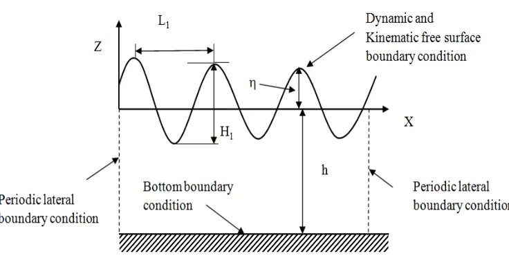
Fig: 2.1 Schematic of the flow domain showing the free surface, normal and tangent vector at the free surface and the horizontal(X) and vertical direction (Z) of the flow domain...27

Fig 2.2 Schematic of the flow domain showing the relation between (elevation), h₀ (when there is no wind action) and h (when wind is acting over the pond)...35

Fig 3. 1 Influence of Surface tension on (a) elevation (Z), (b) flow velocity (Q1) and (c) bottom Stress...67

Fig 3. 2 Influence of Inertia on (a) elevation (Z), (b) flow Velocity (Q1) and (c) bottom Stress ... ...70

Fig 3. 3 Influence of wind direction on (a) elevation (Z), (b) flow Velocity (Q1) and (c) bottom Stress...74

Fig 4.2.1Three types of boundary conditions and the significant wave height and wavelength used in linear wave theory for the calculation of bottom velocity...92

x

xi

NOMENCLATURE

a, b, c Parameters A, B, C Constants

Ca Capillary number

b

C Bottom friction co-efficient

d

C Wind friction co-efficient

D Reference length (transverse direction) (m) Fr Froude number

g Gravitational acceleration



2



m / s

G Gravity number h Depth of water H Depth of water (m)

1

H Significant wave height (m)

L Reference length (streamwise direction) (m)

1

L Significant wave length (m)

xii

N Normal vector

O Order of

p Pressure

P Pressure (Pa)

q Depth integrated velocity/Flow rate



m s2 1



r Wind frequency

R Radius of curvature (m)

D

Re Reynolds number

s Tangent vector

S Tangent vector

t Time

t Traction vector

T Time (s)

T Excess stress

1

T Significant wave period (s)

XX

xiii

ZZ

T Transverse normal stress (N / m2)

XZ

T ,T_ZX Shear stress (N / m2)

u Streamwise velocity component

U Streamwise velocity component



m / s



0

U Wind velocity



m / s



w Transverse velocity component

W Transverse velocity component



m / s



We Weber number

x x-axis position co-ordinate X X-axis position co-ordinate z z-axis position co-ordinate

Z Z-axis position co-ordinate or the magnitude of elevation  Wind direction angle with the positive x-axis (degree)

 Surface tension



N / m



xiv

ε Perturbation parameter/Aspect ratio

 Fluid viscosity



Ns / m2



 Elevation from the reference level

ρ Fluid density



3



kg / m

σ Total stress

 Wind frequency (s)

1

 Angular frequency of the wave (s)

xz

 ,_zx Shear stress

xx

 Stream wise normal stress

zz

 Transverse normal stress

s

 Wind stress

b

 Bottom stress

CHAPTER 1

INTRODUCTION

1.1 General introduction

Shallow or thin-film flow is encountered as a fundamental fluid dynamics problem in various realistic settings such as shallow mine tailings pond, flood wave propagation, atmospheric and ocean modelling, hydraulic jump, tides in ocean, dam break wave modelling, paint and surface coatings, chemical and nuclear reactor design etc. The shallow or thin-film flow with free surface displays a variety of interesting dynamics, since the boundary is deformable. In this case, free surface flow problems are challenging because the flow domain is unknown, and the unknown free surface must be determined as a part of the problem formulation. This is in sharp contrast to most of the fluid mechanics problems, where the flow domain and boundaries are known. Thus, for a free surface flow problem, both the flow field and the free surface shape must be determined in space and time. The reason for studying shallow or thin-film flow i s to gain understanding of a great range of phenomena (like to predict the bottom stress in a shallow mine tailings pond), which in turn allows making predictions in areas of practical importance.

direction is much smaller than the characteristic length scale (L) in the stream wise direction. The flow takes place predominantly in the direction of the longer dimension. Thin-film or shallow flow are the same type of flows and they represent similar flow characteristics. In the present study we have mainly dealt with shallow flow. The influence of inertia, surface tension are examined in this study as from the existing literature (O’Brien & Schwartz 2002, Myers 1998, O’Brien & Van Den Brule 1989), it is found that surface tension is important in small scale and thin-film flow and for capillary waves. Surface tension is also important in porous media and oil medium due to the small capillary number values (http://en.wikipedia.org/wiki/Capillary_number) in these mediums. Several studies (O’Brien & Schwartz 2002, Myers 1998, O’Brien & Van Den Brule 1989) have demonstrated that surface tension is important in thin-film and shallow flow and it cannot be neglected in thin-film and shallow flow. Now we will concentrate our study on shallow flow to determine the bottom stress in a shallow tailings pond.

(L) is much larger compared to the vertical dimension (D). The free surface is given by





ZH X, T in this figure, where X and Z represent the horizontal and vertical direction of the flow domain.

Fig1. 1 Schematic of typical shallow or thin-film flow

be shown that a good approximation to the flow is to replace all of the flow variables by their averages in the vertical direction. The most interesting cases involve a top fluid surface that is free to exhibit the wave phenomenon. Depth-averaged approximations are probably the best known and most widely used in applications relating to the oceans or other large, shallow bodies of water. In this context, the approximation is most often referred to as the shallow-water or thin-film approximation.

1.2. Relevance to reality

The Application of thin-films and shallow flows are very common in nature and technology so an understanding of their mechanics is very important in many real life problems. In this present study we are interested to deal with shallow flow to determine the bottom stress under the influence of periodic wind stress over the flow domain. The present work is of fundamental importance given the significant quantitative role that bottom stress plays to cause erosion and resuspension in a shallow mine tailings pond. Therefore, prediction of the bottom stresses in a shallow mine tailings pond is studied in this study. In general, surface tension has been neglected in most of the studies of shallow water flow. This can be quite reasonably justified, since in most practical applications of shallow flow, surface tension is relatively small. However, there may be still some applications in which surface tension plays a significant role. That is why the problem is formulated with and without the effect of surface tension to see the effect of surface tension on the flow field.

This phenomenon is schematically represented in figure (1.2), where point A represents the position of fluid particle at deep water flow. In this case, the orbital motion of fluid particle decreases rapidly with increasing depth below the free surface. On the other hand, in shallow water flow the elliptical movement of a fluid particle is observed at the bottom of the flow domain (point B represents the bottom position in shallow water flow). Point 1 represents the propagation direction of the flow and (2, 3) represent crest and trough of the flow domain respectively.

Fig1. 2 Motion of a particle in an ocean wave (http://en.wikipedia.org/wiki/Wave_power)

decreases rapidly with depth, while in shallow water flow wave action does not decrease with depth. In shallow water, there is only longitudinal motion at the bottom while longitudinal as well as transverse motions for deep water flow.

Fig1. 3 Flow orbit at the bottom in shallow and deep water flows

http://www.seafriends.org.nz/oceano/waves.htm

In shallow water flow, where depth is less than one-half of the wavelengths, orbits are progressively flattened with depth, and there is little wave drift. Water just above the seafloor cannot move in a circular path and can move only back and forth. Figure (1.4) demonstrates the variation of the flow behavior and characteristics (wave celerity, wave

length), when the waves are moving from deep water flow to shallow water flow through intermediate flow. It is observed from the figure, as the flow moves from deep water flow to shallow water flow, wave orbit changes from circular to elliptical shape.

Mining of metal and uranium ores produces large amounts of reactive sulphide mine tailings which are serious threats and concerns to the environment. One of the approaches used for environmental management of the tailings is the use of shallow water covers, typically up to 2 m. As oxygen is one of the key factors in the oxidation of

Fig1. 5 Schematic representation of tailings pond hydrodynamics (Yanful, E.K., Samad M. & Mian, M.H. (2004))

reactive sulphide minerals present in the tailings, water covers do provide an important control measure. Due to the low diffusivity and solubility of oxygen in water (2e-9m / s 2 and 8.6 g / m at3 25 C) compared to the correspondingly higher values in air (1.78e-5

2

significance in the oxidation of sulphide mine waste (Simms et al. 2001). Water covers can, therefore, be an effective choice in reducing tailings oxidation and resuspension.

Mine tailings ponds are normally designed to minimize the wind-induced bottom erosion and sediment resuspension. Figure (1.5) shows the representation of a tailings pond hydrodynamics. In this figure, the formation of the wind induced bed shear stress and bed shear stress due to return current is illustrated. This figure also shows the wind action over the flow domain, which induces bottom stress to cause resuspension of the tailings. The ponds are constructed with a minimum depth of water cover.

Deep water covers appears to be less attractive option to mine operators due to concerns on the long-term stability of reservoirs from hydrostatic pressures, the high costs of construction including efficient flood control systems and its maintenance, and the attendant monitoring of the structure and water quality (Yanful, et al, 2004). Shallow water covers, compared with deeper ones can also provide the twin benefits of limiting oxygen diffusivity and solubility, thus dampening AMD production and metals release. For shallow water flow, wave action is the dominant force in creating shear while it is the return current in deep water flows.

1.3 Literature review

Thin-film flow has mostly been examined for Newtonian fluids (Brourgin 1997; Kistler & Schweizer 1997). Generally most studies involve either gravity driven or surface-tension-driven flow. A simple and obvious example of thin-film flow is the flow of a (thin) raindrop down a windowpane under the action of gravity. Typically, the flow velocity in directions perpendicular to the substrate (the window-pane) is much smaller than the main flow velocity along the windowpane. The most suitable approach for modeling such flows is via the momentum equation (the Navier-Stokes equations in the case of a Newtonian liquid). The approach taken here will be to exploit the existence of the small aspect ratio ( D

L

  ) to expand the solution in a perturbation series in powers of . In doing so thin-film or long wave approximation is developed (Benney 1966) with the advantage that analytic solutions will often be possible and where this is not feasible, the reduced numerical problem will be greatly simplified (Tuck & Schwartz 1990). The approximation has much in common with classical lubrication theory (Acheson 1990) and is thus also referred to as the lubrication approximation. In the next section some previous studies on surface tension driven thin-film flows are described.

problems with a free surface are given by Benney (1966) without surface tension and by Atherton and Homsy (1976) where surface tension is included.

In Encyclopedia of Surface and Colloid Science (2002) by O’Brien & Schwartz , it was described that it is the common practice of many authors to rescale the surface tension terms so that they are O (1), by assuming that 3/ CaO 1

 

, (where Cais the capillary number). It was assumed whether the rescaling is technically correct depends on the particular parameter values in the problem under consideration but the idea is that even if these terms are everywhere small, including them will still give a correct approximation to leading order. This approximation usually has the desirable effect of making the numerical technique more stable. The study was more concerned with the flow on centimeter-scale objects rather than meter-scale objects.

Stone (2002) has demonstrated that waves in thin-films or shallow flow behave differently than waves in deeper flow. This is because of the high viscous stresses, low impact of inertial forces as the lubrication assumption remains the basis for the simulation of thin-film flow where the inertial effects are neglected (Mazouchi & Homsy 2001), low velocity, and influence of surface tension at the small scales involved. In this paper, the governing equations of thin-films are derived from the Navier-Stokes equations. The behavior of thin-films can be described by the lubrication approximation. This approximation was used to find the behavior of small disturbances as they evolve in space and time. In order to extend the results to faster waves and deeper liquid, inertial terms should be included as inertial effect is important in deeper liquid. By doing this, one could check that the behavior approaches the well known behavior of waves in deeper liquids. Stone considered the time-dependent motion of thin-filmsin cases where viscous effects are significant. This topic may be considered naturally under the theme "reactive flows" since changes in surface tension produce fluid motions this is a response that occurs at fluid-fluid interfaces.

space and time. They have also explored the effect of gravity, showing that it could result in the disappearance of capillary ridges. The stability of the latter was considered in a subsequent article by Kalliadasis & Homsy (2001).

Mazouchi & Homsy (2001) have compared the solution of the two-dimensional flow to their earlier thin-film based solution. This comparison indicated that the thin-film hypothesis remains valid even in the presence on steep topographic variation. Mazouchi & Homsy (2001) attributed this validity to the smoothing role that surface tension effects tend to play. Their study was limited, however to surface-tension dominated inertia less flows.

of authors demonstrated lubrication theory to be surprisingly accurate for modelling purposes even for cases where it is not strictly valid, as for the flow over shallow trenches.

Siddique and Khayat (2002) have shown that in classical lubrication theory the Navier–Stokes equations are reduced to the Reynolds equation under the assumption that the inertia forces are negligible compared to the viscous forces. This conventional thin-film theory is valid for small Reynolds number flow. They also addressed that recently, owing to some practical applications, the need to include inertia effects has arisen because of the increasing number of lubrication problems that involve moderately large Reynolds number.

under the influence of viscosity and surface tension at a moderate Reynolds number. Some literatures on the bottom stress determination in a shallow mine tailings pond are discussed in the next section.

The study of resuspended flooded mine tailings pond has been extensively examined previously in the literature. However, fundamental work on this analysis is limited. In addition, most published work on prediction of the bottom stress for reactive sulphide rich tailings pond is based on empirical, predictive methods. Most studies focused on Airy (linear wave) theory to predict the flow behavior in the shallow mine tailings pond. There are many studies devoted to the modeling and simulation of the resuspended flooded mine tailings. Most importantly, resuspension in mine tailings pond has been predominantly examined from the empirical methods (Samad and Yanful 2005), (Yanful and Catalan 2002) and to a much lesser extent from the fundamental fluid equations (conservation of mass and momentum) considering the viscous and surface tension effects.

capillary waves and other very short waves). This theory is only applicable for a smooth and impermeable bottom. Therefore, the limitations of this theory sometimes limit its use in the real world problems.

Wind induced bed shear stress in a closed water body is made of two parts (i) bed shear stress due to waves and (ii) bed shear stress due to circulatory currents. However, it is not clear from the published literature how the waves and currents should be handled in enclosed shallow water bodies to obtain the total bed shear stress exerted on the bed surface by the wind action, which is required for analyzing resuspension and sediment transport processes. In many studies the current induced bed shear stress in shallow water is either considered too small to contribute to resuspension (Luettich et al. 1990; Bailey and Hamilton 1997; Cozar et al. 2005) or estimated using theoretical and empirical approaches developed under laboratory conditions such as those developed by Wu and Tsanis (1995) and Yang (2001). Previous studies (Yanful and Catalan 2002) ignored the current induced bed shear stress in a tailings pond, assuming it to be only 10% of the total bed shear stress. However, Samad and Yanful (2005) later found that the bed shear stress due to currents often exceeded 20% of the total bed shear stress. In their study, they also calculated total bed shear stress as a linear addition of both wave and current induced bed shear stresses.

Ridd 1996; Jin and Ji 2004). In order to include wave-current interaction in the total bed shear stress calculations, actual field measured current data is needed. In most of the tailings pond studies, information about actual currents data have been missing and currents were empirically calculated as counter currents.

In most studies so far conducted on the tailings ponds, the total bed shear stress was taken as a simple linear addition of the shear stress contributions from waves and currents (Yanful and Catalan 2002; Samad and Yanful 2005; Kachhwal et al. 2010). In these studies near bed, currents were assumed as counter current flow in opposite direction to wind based on the Wu and Tsanis (1995) theoretical model developed for pure currents in absence of waves. In the presence of both waves and currents, linear addition may not be accurate especially for strong currents and may underestimate the total bed shear stress. The empirical approaches used to estimate the wind induced currents in these tailings pond studies do not provide any information on current directions and circulation patterns. The lack of field measured wind induced current data in small tailings pond is a constraint. Kachhwal (2011) measured real time wind induced currents in a tailings pond and studied the effect of wave-current interaction on total bed shear stress. It is clear from his results that currents significantly contribute to total bed shear stresses to cause resuspension in a tailings pond.

tailings, and sediment trap measurements at the Heath Steele Upper Cell tailings pond, New Brunswick, Canada. The prediction of resuspension is compared to the field measured resuspension of tailings under varying water cover depth at a site based on the results, it is concluded that bed shear stress was higher in shallower water covers.Under the maximum sustained wind speed of 10 m/s observed at the study site, the predicted total shear stress exceeded the upper and lower bounds of the critical shear stress in parts of the tailings pond, where the water cover was less than 1.18m and 1.34 m deep, respectively. By comparison, field measurements of tailings resuspension using sediment traps suggested that resuspension occurred primarily in areas where the water cover depth was 1 m or less.

was still observed at these sites as already discussed. Thus, it might be inferred that, even with the use of SMB equations for the design of water covers for new mine-tailings sites, resuspension might still be expected at higher wind speeds, leading to oxidation and potential deterioration of water quality.

1.4 Motivation:

For small inertia flow of a Newtonian film, Benney’s (1966) long wave (LW) approximation is often used. At first glance, the LW approximation appears to be a suitable choice for the modeling of thin-film or shallow flow. However, the LW approximation becomes seriously limited in the presence of moderate or high inertial effect (Chang 1994). For a Newtonian film, the LW approximation at Re >> 1 is typically not valid, and it is generally found that in this case, inertial effects are better represented using the boundary-layer (BL) formulation. In this present study, boundary-layer formulation is found using the suitable scaling for typical shallow flow. The present study is considered for moderately large inertial effects.

Free surface and interfacial flows are inherently complicated because of the unknown position of the free surface or interface, which must be determined as a part of the problem. The understanding of the thin-film or shallow flow initiated by the wind action remains challenging, despite the continuous development of new solution techniques and the advent of powerful computational platforms due to the fact that computational domain is unknown a priori along with the unknown position of the free surface. So it is quite challenging to assume the correct boundary conditions to solve the problem.

assumed at the both lateral boundaries as the flow domain is assumed confined and fixed. The bottom boundary condition remains the same in the present formulation as of linear theory that the flow velocity at the bottom is zero due to no- penetration condition in the transverse direction.

assumed to be viscous but the surface tension effect is neglected while in our formulation we have considered the surface tension as well as viscous effect in a shallow or thin-film domain.

In the present model the wind is taken at an angle

 

 with the x-axis of the flow domain. But in most of the existing studies (Fenton 2010, Matthews et al. 1996, Lick 1976) it is found that, wind acts parallel over the shallow flow domain. Although in most of the existing studies (Lick 1976, Fenton 2010) the angle is taken as zero



 0



but in this present study using wind at an angle

 

 is described as an alternative way of describing wind condition over the shallow pond which resembles with the existing wind stress expression when the angle is zero. Although we have tried to compare our results with the existing linear theory results but the wind situation in two cases are not same. As in linear theory, wind is taken as constant while in our model we have assumed periodic wind stress with time. But if we assume the wavelength to be infinite then the wind condition in our formulation can be assumed constant as of linear wave theory. We have tried to find a behavioral trend of the bottom stress for different water depth in a tailings pond.

cases are considered in this study, with and without the effect of surface tension on the flow field. The influences of surface tension, inertia and wind direction on the flow field are explored in this present study. Most published work (Yanful and Catalan 2002, Samad and Yanful 2005) on prediction of the bottom stress for tailings pond is based on empirical, predictive methods where the linear theory is used to predict the flow behavior in a shallow tailings pond.

The main focus of this present study is to predict the bottom stress starting from the fundamental equations (conservation of mass and momentum) for a given wind speed and water depth in the presence of inertia and surface tension in a tailings pond. Starting with the fundamental equations, the equations are converted to boundary-layer equations for shallow water flow using the suitable scaling method. Insertions of the effect of ambient wind condition and bottom shear stress are done to formulate the problem for the flow field. A small perturbation method is used to solve the problem and finally, the expressions for the elevation, flow velocity and bottom stress are found as the solution of the problem. The predicted bottom stress values from the present study using different water depths for a particular wind velocity, show good agreement with the existing theoretical (linear theory) and the experimental (Yanful and Catalan 2002) bottom stress values although the wind condition in the present model is not same as of linear theory.

CHAPTER 2

GENERAL PROBLEM FORMULATION

In this chapter, the governing equations are introduced, including the suitable scaling of the constitutive equations as well as the boundary conditions for shallow water flow. The solution procedure is also described in this chapter in some detail.

2.1 Problem formulation and boundary conditions for shallow water flow

The fluid examined in this study is assumed to be an incompressible fluid, which has the fluid properties of density and viscosity. The problem is examined in the (X, Z) plane. Regardless of the nature of the fluid, the continuity and the momentum conservation equations must hold. For an incompressible fluid, the conservation equations are:

0

 U , (2.1.1)



_T



,

 U  U U   σ g (2.1.2)

is denoted by nands. Equations (2.1.1-2.1.2) for conservation of mass and momentum are expressed in dimensional form as

Fig: 2.1 Schematic of the flow domain showing the free surface, normal and tangent vector at the free surface and the horizontal(X) and vertical direction (Z) of the flow domain.

n s

X Z = H(X, T)

U W 0,

X Z

 _ _

  (2.1.3)

XX ZX

T T

U U U P

U W ,

T X Z X X Z

 

   

 

_   _   

     

  (2.1.4)

XZ ZZ

T T

W W W P

U W g,

T X Z Z X Z

 

   

 

_   _     

     

  (2.1.5)

where all the terms are in dimensional form. Here, U and W are the stream wise (X direction) and vertical (Z direction) velocity respectively and P is the hydrostatic pressure in the shallow pond. Free surfaces occur at the interface between two fluids, such interfaces require two boundary conditions to be applied (i) A kinematic condition which relates the motion of the free interface to the fluid velocities at the free surface and (ii) a dynamic condition which demonstrates the force balance at the free surface.

If the free surface is given by f f X, Z, T





0, then its normal is given by N f and

the unit normal is given by f f

n  

 , the plus and minus signs correspond to n pointing away from and toward the free surface, respectively. In this formulation, it is taken as

f . f     n

Now, for this problem the free surface is given byZH X, T





f  Z H X, T





, so

X

f H ,

X

X Z

2 2

X X

H 1

n n .

H 1 H 1

    

 

n i k i k (2.1.6)

As the unit tangent vector remains at 90 degree angle to the unit normal vector, therefore, the expression for the unit tangent vector becomes

X

X Z Z X

2 2

X X

H 1

s s n n .

H 1 H 1

     

 

s i k i k i k (2.1.7)

The dynamic boundary condition requires the stress to be continuous across the free surface which separates the two fluids (air and water). The traction exerted by one fluid (1) on another fluid (2) is equal and opposite to the traction exerted by fluid (2) on fluid (1). As surface tension is included in this study, the dynamic boundary condition is also modified and traction at the free surface is given by

,  

t n (2.1.8)

where tis the traction vector at the free surface, _{is the surface tension and} nis the unit normal vector at the free surface. Note that, the curvature can be positive or negative. It is known that the

 

 is the reciprocal of the radius of curvature (R) and expressed as





XX 3 2 2 X H 1 . R 1 H      (2.1.9)

equation (2.1.8), the scalar product of the traction vector with the unit tangent vector at the free surface gives

.    

t s n s (2.1.10)

As the unit normal and the unit tangent vector remains perpendicular to each other, their scalar product is zero. n s 0. Using this value in equation (2.1.10) leads to

0,

 

t s (2.1.11)

where tis the traction vector at the free surface and it is substituted by the scalar product of the total stress σ and the unit normal vector. In other words, t σ n,using this expression into equation (2.1.11) reduces to



σ n s  



0. (2.1.12)

Now, the total stress is replaced by σ PI T , where Tis the excess stress and Iis the identity matrix. So, equation (2.1.12) becomes



 P



  0.

 

 I T n s (2.1.13)

The scalar product of the identity matrix and the unit normal vector to the free surface is equal to the unit normal vector at the free surface. In other words, I n n,using this value into equation (2.1.13) leads to

P 0.

The first part of equation (2.1.14) is zero, as there is a scalar product between the unit normal and unit tangent vector to the free surface (they remain perpendicular to each other). In other words, n s 0.Using this value into equation (2.1.14) reduces to

0.   

s T n (2.1.15)

Expanding equation (2.1.15) over X, Z; the equation (2.1.15) becomes,





X X XX X Z Z X XZ Z Z ZZ

s n T  s n s n T s n T 0.

Inserting the components of the unit normal and the unit tangent vector (from equations 2.1.6-2.1.7) in X and Z direction leads to





X

XZ ₂ ZZ XX

X

H

T T T 0.

1 H

  

 (2.1.16)

Similarly, the traction at the free surface in the normal direction is found by taking the scalar product of the traction vector with the unit normal vector to the free surface. Using equation (2.1.8), the scalar product of the traction vector with the unit normal vector at the free surface gives

,    

t n n n (2.1.17)



σ n n   



. (2.1.18)

Now, the total stress is replaced by,σ PI T , where Tis the excess stress and Iis the identity matrix. Inserting this expression into equation (2.1.18), equation (2.1.18) reduces

to,_



 PI T n



 _  n . (2.1.19)

As it is known, I n n,inserting this value into equation (2.1.19) leads to

P .

       n n n T n (2.1.20)

There is a scalar product between the two unit normal vectors to the free surface in equation (2.1.20) and the value is one. In other words, n n 1.Using this value into equation (2.1.20) reduces to

P    n T n . (2.1.21)

Expanding equation (2.1.21) over X, Z; equation (2.1.21) becomes,

2 2

X XX X Z XZ Z ZZ

P n T 2n n T n T  .

Inserting the components of the unit normal vector from equation (2.1.6) in X and Z direction and using the expression 1

R

  leads to

X XZ ZZ

P H T T .

R



The kinematic boundary condition describes the flow velocity in the transverse direction, which is equal to the change of surface height with time. It relates the motion of the free interface to the fluid velocities at the free surface.

H T X

dH

W H UH .

dT

   _(2.1.23)

In principle, equations (2.1.3-2.1.5) can be solved subjected to the boundary conditions (2.1.22-2.1.23). However, given the small depth of shallow water flow, the governing equations are simplified further and converted to boundary-layer equations for shallow water flow, which is described in the next section.

2.2 Boundary-layer equations for shallow water flow

D , L

  0

D

U D

Re  ,

 0

U Ca ,

 3 We , Ca   (2.2.1)

where U₀ is the wind velocity measured at a reference height (usually 10 meter) over the shallow pond, γ is the surface tension and the Reynolds number is based on the characteristics length scale (D).

In this study, the ratio of the water depth to the length of pond is too small



 1 ,



which is named as the aspect ratio. Thus, is taken as the perturbation parameter to reduce the problem to the boundary-layer type. The scaling of the position co-ordinates, velocity, pressure, time and stress components are obvious, leading to (where in scaling of time,  is used known as wind frequency)

0 U u U  , 0 W w D U L

 , t T, x X L  , Z z D  , 0 2 P p U L  _      

, h H, D  xx xx 0 T , U L   _ zz zz 0 T , U L    XZ ZX xz zx 0 0 T T . U U D D     

Fig2.2 Schematic of the flow domain showing the relation between (elevation), h₀

Figure (2.2) illustrates the flow domain in non-dimensional form, whereh₀

represent the fixed water level without the wind action and h represent the depth of water when wind is acting over the flow domain. Three types of boundary conditions (bottom boundary condition, lateral boundary condition and free surface boundary condition) are used to solve the problem. Wind creates drag on the water surface which is termed as the wind boundary condition on the water surface. Though in most of the existing studies wind acts parallel to the length of the pond but in our formulation we have taken that wind acts at an angle  to the positive x-axis of the flow domain. In this figure (2.2), x and z represent the horizontal (streamwise) and the vertical (transverse) direction of the flow domain, where D and L are the characteristics vertical and horizontal length scale of the shallow pond respectively. Upon introducing dimensionless variables from equation (2.2.2) into equations (2.1.3-2.1.5), and ignoring the terms of O

 

2 or higher, the relevant equations for the problem reduce to non-dimensional form as

u w

0,

x z

 _ _

  (2.2.3)

zx D

u u u p

Re r u w ,

t x z x z



   

 

 _   _  

    

  (2.2.4)

p G, z

 _{ }

 (2.2.5)

where in the governing equations,

0

L r

U



 is the dimensionless frequency of the wind

wave and  is the frequency of the wind cycle over the flow domain.

2 0 D g G U   

Gravity number which is the ratio of the Reynolds number to the Froude number.

D Re G

Fr



The reduced conservation equations are derived using the suitable scaling, where the terms of O (ε2) or higher are excluded from the problem formulation. As it is known that the boundary-layer flow is a shear dominated flow, so after scaling, it is found that the normal stresses are negligible as they are of O (ε2).

The scaling method is applied to the dynamic boundary condition (equation 2.1.16) in the tangential direction. The boundary condition is expressed in non-dimensional form as









2 x

xz ₂ zz xx

x

h

0.

1 h



     

  (2.2.6)

Ignoring the terms of O

 

2 in equation (2.2.6), results in the vanishing of the shear stress at the free surface as

xz 0.

  (2.2.7)

The radius of curvature (equation 2.1.9) in dimensional form is expressed as





XX 3 2 2 X H 1

, R

1 H

    

where

 

R is the radius of curvature of the free surface and it is non-dimensionalized (r_c) using the horizontal length scale (L). Using the scaling r_c R,

L

 the radius of curvature (equation 2.2.8) is expressed in non-dimensional form as

x 2 3 c 2 2 x D h 1 _L . Lr D 1 h L      _{ }   _{  }   _{ }    (2.2.9)

Inserting the expression D

L   as the aspect ratio, expression (2.2.9) becomes





x 3 c ₂ 2 2 xx h 1 _L . Lr 1 h        (2.2.10)

Ignoring the term of O

 

2 in expression (2.2.10), expression (2.2.10) reduces to

x c 1 h . Lr L 

    (2.2.11)

Now, the non-dimensional dynamic boundary condition in the normal direction is found,

when the scaling is applied to equation (2.1.22). The expressions from equations (2.2.7

0 0 x zz

2

U U h

p . L L L            

  (2.2.12)

Inserting the expression of capillary number from expression (2.2.1) into equation (2.2.12), equation (2.2.12) reduces to

x zz 2 h p . Ca   _{ } _{ }   

  (2.2.13)

So, the expression for the pressure at the free surface becomes





2 3 x

zz

h p x, z h, t

Ca 

     . (2.2.14)

This is the dynamic boundary condition in the normal direction at the free surface. The expression for the pressure is found by integrating equation (2.2.5) with respect to z as

 

p Gz c x, t _{, (2.2.15)}

where c x, t is an integration constant. Now, substituting the expression of the pressure

 

at the free surface from expression (2.2.15) leads to

 

3

2 x

zz

h

Gh c x, t . Ca



      _(2.2.16)

Now, the value of c x, t is found as

 

 

2 3 x

zz

h

c x, t Gh.

Ca 

Inserting the expression ofc x, t into equation (2.2.15), the expression of the pressure

 

becomes





2 3 x

zz

h

p G z h .

Ca 

      _(2.2.18)

Ignoring the term of O

 

2 in equation (2.2.18), equation (2.2.18) reduces to





3hx

p G z h .

Ca 

   _(2.2.19)

Though in the problem formulation the terms of O (ε2) or higher is neglected, the second term in equation (2.2.19) is not neglected as it is assumed that the capillary number is too small to compensate the effect of O (ε3). Differentiating the pressure with respect to x, equation (2.2.19) gives

 

3

x

p h

G h .

x x Ca x

 _{ }  _  

   (2.2.20)

Now, h is the depth of water when wind is acting over the shallow pond and  is the elevation from the reference level (fixed water level, the level of water when there is no wind action over the shallow pond). So, the expression of h becomes

h  1 . _(2.2.21)

h x x  _    , 2 2 2 2 h x x  _  

  and

h .

t t

 _

  (2.2.22)

Substituting the expressions of h

x



 and

2

2 h

x



 into equation (2.2.20), gives the value of

the pressure derivative as

3

x x xx

p

p G .

x Ca

 _{    }  _

 (2.2.23)

The scaling method is then applied to the kinematic boundary conditions (2.1.23), the kinematic boundary condition at the free surface (z = h) is expressed in non-dimensional form as

0 h

0 0

uU

D h D h

w .

U t U L x

  

 

    (2.2.24)

Substituting the expression of D

L   into equation (2.2.24), equation (2.2.24) reduces to

h 0

L h h

w u .

U t x

  

 

  (2.2.25)

Introducing a new dimensionless parameter (r) into equation (2.2.25), where 0

L r

U   is

the dimensionless frequency of the wind wave over the shallow pond. Simplifying equation (2.2.25) leads to

h t x

Similarly, the kinematic boundary condition at (z = 0) is expressed in non-dimensional form as

0

w 0. (2.2.27)

In this section, as the depth of shallow water flow is very small, using the suitable scaling; the equations are converted to boundary-layer equations for shallow water flow. In the next section, the effects of wind and the bottom are incorporated in the governing equations which come through the wind and bottom stresses to formulate the problem.

2.3 Incorporation of the wind conditions and the bottom shear stress

In this section, the influence of the wind action and the effect of bottom are incorporated in the governing equations. The influences of the wind action and the bottom of the pond come through the wind and bottom stress terms in the boundary-layer equations for shallow water flow.

Wind boundary conditions:

(Wu’s equation as presented in the RMA2 Users Guide (U.S. Army Corps of Engineers-Waterways Experiment Station, 1996) and Van Dorn’s equation (Dean and Dalrymple, 1991)).

Oscillatory wind is the main driving force to cause resuspension in a shallow tailings pond. The wind stress is directed at an angle

 

 _{to the positive X-axis of the} flow domain. Matthews et al. (Appl. Math. Modelling, 1996) have used  0 to express the periodic wind forcing acts in the X direction over the flow domain. So, using  0 in the wind stress expression by (Mclnerney, Teubner and Noye 2010) resembles the wind stress expression by Matthews et al.

There are several expressions available in the literature by which wind stress can be expreesed.Wind stress can be expressed by Coastal and Ocean Engineering (Fenton 2010) as,

2 d 0

C U    ,

where C_dis the drag coefficientC_d .0075 .000067U ₀, in which U₀ is the wind speed at a height of 10m, and  is the density of air. The actual speed of the ocean current is a small fraction of the wind speed, roughly 3-5%.

observations. The formula or the expression for wind stress given by (Lick 1976) is as follows,

n 1

d 0 0

C U U ,   

where C_d is a drag coefficient,  is the density of the air, U₀ is the wind velocity measured at 10 m height above the water surface, and n is an empirically determined exponent not necessarily integer. Wilson (1960) has analyzed the data from many different sources and has given a best fit to the data. For U₀ in units of cm/sec, Pa in units of gm/cm3, and  in units of dynes/cm2, Wilson suggests a value of n=2 and C_d

=0.00237 for strong winds and 0.00166 for light winds. From a comparison of field data and results of numerical models, Simons (1974) suggests values of n=2 and C_d=0.003.

Though in most of the existing studies wind acts parallel over the length of the shallow tailings pond but we have assumed that the wind acts at an angle  to the positive X-axis of the flow domain and used the expression of the wind stress by (Mclnerney, Teubner and Noye 2010) in the momentum equation. In the X-momentum equation (2.1.4),T_{ZX Z H} T_ST cos cos₀ 

 

T is the wind stress with magnitude T ₀ and frequency  _{(which is the frequency of the wind cycle).}T_{ZXZ H} T_S is simply a representation of wind stress with

- Maximum magnitude of T₀ C U_{d 0}2 ,

- The wind is directed at an angle of alpha

 

 to the X-axis. (The X-component of the wind corresponds to cos).

- The wind stress is not meant to be realistic. The simplicity of this equation enabled us to produce the analytic solution. We have tried to use this expression as a different approach to express the wind stress working over the flow domain. By setting  0 and ignoring time dependency it resembles the traditional or realistic wind force acts parallel over the flow domain.

- The wind stress is assumed to be periodic with time to observe the effect of the flow field under the periodic wind condition.

- The wind is taken at an angle with the X-axis of the flow domain. But in most of the existing studies it is found that, wind acts parallel over the shallow flow domain. So using wind at an angle

 

 can sometimes limits the use of the present wind stress expression in real life problems. Now the wind stress expression will be incorporated in the X-momentum equation (2.1.4) as,





 

ZX _{Z h} s 0

T _ T T cos cos T , (2.3.1)



  



  

2

d 0

zx _{z h} s d D

0

C U

cos cos t C Re cos cos t . U

D





    _    (2.3.2)

Incorporation of bottom stress:

Similarly, in the X-momentum equation (2.1.4) _{ZX b} Z 0

T _ T is the bottom stress in dimensional form. It is commonly expressed empirically using the quadratic law, where C is the bottom friction co-efficient. Typical value of C_{b b} is ofO 10

 

3 . The bottom stress (Tsanis & Saied 2005) is expressed in dimensional form as

ZX _{Z 0} b b

T _ T  C U U , (2.3.3)

where is the density and U is the flow velocity of water in dimensional form. The bottom stress after the scaling is expressed in non-dimensional form as

2

b 0 0 2

zx _{z 0} b b D

0

C u U U

C Re u . U

D





    _  (2.3.4)

The depth integrated velocity (flow rate) qis expressed as

h

0

q



udz. (2.3.5)

h

0

qu dz



uh. (2.3.6)

So, the expression of the bottom stress (equation 2.3.4) in terms of depth integrated velocity (flow rate) is expressed as

2 2

zx _{z 0} b b D b D ₂

q

C Re u C Re .

h



     (2.3.7)

Now, integrating equation (2.2.3) over the depth of water (between 0 to h), the continuity

equation becomes h 0 u w dz 0. x z    _  _ _{ }   



(2.3.8)

After integrating equation (2.3.8) with respect to z, equation (2.3.8) reduces to

h

h 0

0

u

dz w w 0.

x   _{   } _   



(2.3.9)

Now, using the Leibniz rule, the value of the term

h 0 u dz x    _   



is determined as

h h

0 0

u h

dz udz u .

x x x

  

 _{  }

_  _{ }

 





(2.3.10)

As u is independent upon z, the following expression is found as

 

h h

0 0

udz u dz uh .

x x x

 _  _ 

Inserting the expression of h 0 udz x 





from equation (2.3.11) into equation (2.3.10) leads to

 

h

0

u h

dz uh u .

x x x

  

 _{  }

_  _{ }  



(2.3.12)

The values of the terms

h 0 u dz x    _   



,



w , w_{h 0}



found from equations (2.3.12, 2.2.26-2.2.27)

are inserted into equation (2.3.9) gives

 

uh uhx rht uhx rht

 

uh 0.

x x

 _{    }  _

  (2.3.13)

The value of the depth integrated velocity (q) from equation (2.3.6) is inserted into equation (2.3.13), and using the expression of h

t



 from equation (2.2.22) into equation

(2.3.13) reduces to

q

r 0.

t x

 

 

  (2.3.14)

Now, equation (2.2.4) is integrated over the depth of water between 0 to h. From shallow water approximation it is known that u is independent upon z, setting u 0

z

 _  into

equation (2.2.4), equation (2.2.4) reduces to





D t x zx _{z h} zx _{z 0}

p

Re rhu uhu h .

x  



       

Substituting the expressions of pressure gradient, wind and bottom stress from equations (2.2.23) and (2.3.2-2.3.4) into equation (2.3.15) yields





2





2

D t x ₂ d D b D ₂

q

Re rhu uhu Gh Weh C Re cos cos t C Re ,

x _{x h}

           _ (2.3.16) where 3 We Ca 

 is the Weber number and Ca is the capillary number. Dividing the both

side of equation (2.3.16) with Re_Dresults in



t x



2₂ d D





b D 2₂

D

1 q

rhu uhu Gh Weh C Re cos cos t C Re .

Re x _{x h}

 _{  } 

  _     _

 _  _{ }

(2.3.17) From equation (2.3.13) it can be shown that

 

t t x x

rh uh rh uh hu 0.

x



    

 (2.3.18)

Multiplying equation (2.3.18) with u gives





t x x

urh u uh hu 0. (2.3.19)

Adding equations (2.3.17 and 2.3.19) results in





2 2

2

t t x x ₂ d D b D ₂

D

1 q

urh rhu 2huu u h Gh Weh C Re cos cos t C Re .

Re x _{x h}

 _{  } 

    _     _

 _  _{ }

Substituting the expressions of

 

ruh ruh_t rhu_t t

 _{ }

 and

 

2 2

x x

u h u h 2huu

x

 _{ }

 into

equation (2.3.20) gives

 

 

2 2





2

d D b D

2 2

D

1 q

ruh u h Gh Weh C Re cos cos t C Re .

t x Re x _{x h}

 

    

  _     _

   _  _{ }

(2.3.21)

Inserting the expression of depth integrated velocity (flow rate) from equation (2.3.6) into equation (2.3.21) leads to





2 2 2

d D b D

2 2

D

q q 1 q

r Gh Weh C Re cos cos t C Re .

t x h Re x _{x h}

     _  _ _  _{  }           _{ }  _  _{ } (2.3.22)

The boundary conditions at the two lateral boundaries of the shallow pond are given by













q x 0, t q x 1, t 0 , x 0, t 0

   _{ } 

   _ (2.3.23)

2.4. Solution Procedure

In this section, the equations (2.3.14 and 2.3.22) are solved using a small perturbation approach subjected to the boundary conditions (2.3.23). A third order ODE is solved to find the three roots of the ODE. Using these three roots, the expression of the elevation is found by solving the governing equations. With the help of the expression of the elevation, the expression of the flow velocity is found using the continuity equation. The expression for the bottom stress is found using the empirical relation (2.3.4), where the bottom stress depends on the flow velocity. The expressions of the flow field (elevation, flow velocity and bottom shear stress) are found as the solution of the governing equations (2.3.14 and 2.3.22). In the present study, the surface tension component is not neglected and the change in the flow behavior due to surface tension is also studied.

A small perturbation approach is used to solve equations (2.3.14 and 2.3.22), where it is assumed that the elevation is an order of magnitude smaller than the depth of water. Solutions of equations (2.3.14-2.3.22) are of the following form

n 1

n 1

n 1

,



 



     (2.4.1a)

n 1

n 1

n 1

q q q ,







   (2.4.1b)

   







 



1

2 3

1

1 1 1

1

1 1 1

1 1 1 1 ... 1 1 O .

h 1 1 1

       _   _                  (2.4.2)

Now, using equations (2.4.1a and 2.4.1b) to formulate the problem for first order solution, equation (2.3.14) yields

1 q1

r .

t x

 _{ }

  (2.4.3)

It is known from equation (2.4.1b), that the depth integrated velocity is ofO

 

 so, the bottom stress (equation 2.3.10) having O

 

2 is neglected for first order solution (as in

problem formulation the terms of O

 

2 or higher are neglected). Therefore, for first order solution equation (2.3.22) becomes





2

d D

1 1 1

2 D

C Re cos cos t

q 1

r Gh Weh .

t Re x _x

 _ 

 _  _   _

 

 

  _  _  _ (2.4.4)

Using equation (2.4.1b) to insert the expression of h, and omitting the terms of O

 

 yields the first order solution as





2

d D

1 1 1

2 D

C Re cos cos t

q 1

r G We .

t Re x _x

 _ 

 _  _   _

 

 

  _  _  _ (2.4.5)









1 1

q x0, t q x1, t 0, (2.4.6)





1 x 0, t 0.

   (2.4.7)

Now, equation (2.4.5) is differentiated with respect to x, leads to

2 3

1 1 1

2 3

D

q 1

r G We .

x t Re _{x x}

 

    

  _{    }

  _{ }

 _  _  _{   } (2.4.8)

Inserting the expression of q1

x



 from equation (2.4.1.3) into equation (2.4.8) gives

2 3

1 1 1

2 3

D

1

r r G We .

t t Re _{x x}

 

    

 _ _{   }

  _{ }

     _   _ (2.4.9)

Dividing equation (2.4.9) with the Weber number (We) leads to

3 2 2 2

1 1 D 1

3 2 2

r Re G

0.

We We

x x t

  _   _   _

   (2.4.10)

Introducing two new parameters in equation (2.4.10) as

G a, We  2 D r Re b. We  _ (2.4.11)

Inserting these new parameters into equation (2.4.11) leads to

3 2 2

1 1 1

3 a 2 b 2 0.

x x t

  _   _   _

The boundary conditions are also changed and expressed in terms of first order elevation. Using the boundary condition (2.4.6) for first order solution, it is found that q1 0

t

 

 . So,

substituting this expression into equation (2.4.5) results





2

d D

1 1

2

C Re cos cos t

G We .

x _x

  _   _

 _  (2.4.13)

Dividing equation (2.4.13) with the Weber number (We) and substituting G a We  reduces to





2 d D 1 1 2

C Re cos cos t

a . x We x    _  _{ }    (2.4.14)

Now, the boundary conditions are expressed in terms of first order elevation as





2 2

d D

1 1 1 1

2 2

x 0 x 1

C Re cos cos t

a .

x x We

x _ x _

_{  }  _{  }  _

    

   

 _{ }   _{ }  _

    (2.4.15)

The third boundary condition is found from equation (2.4.7) as

1 x 0 0.

  (2.4.16)

The most general form of ₁ as a solution of equation (2.4.12) is expressed as

 

1 Z x cos t.