Distributed Estimation Based on Prior Information

(1)

Distributed Estimation Based on Prior Information

Magdi S. Mahmoud and Haris M. Khalid∗†

March 15, 2013

Abstract

In this paper, we propose an approach for distributed estimation algorithm using Bayesian-based forward backward (FB) Kalman filter (KF) used on a stochastic singular linear system. The approach incorporates generalized versions of KF presented for cases with complete or incompletea-priori in-formation with bounds, followed by estimation fusion for these cases. The proposed approach is then validated on a coupled tank system to ensure its effectiveness.

Keywords: Kalman filtering, Bayesian approach,a-priori information, stochastic singular linear system, distributed estimation, coupled tank system.

1 Introduction

In this era of highly technical environment, a strict surveillance unit is required for an appropriate super-vision. Distributed and decentralized estimations are the solutions to such a high profile strategy. It often utilizes a group of distributed sensors which provide information of the local targets. The information is processed locally at each node, there is no central data-processing node here. This architecture is useful for large flexible and smart structures e.g. condition and health monitoring of aircraft, spacecraft, huge auto-mated plants, large sensor networks and chemical industries. The classic work of Rao and Durrant-Whyte [1] presents an approach to decentralized KF which accomplishes globally optimal performance in the case where all sensors can communicate with each other. Sensor noises of converted systems cross-correlated,

∗_Manuscript_{MsM-KFUPM-PrKnowEst-IET-SP[R-II].tex}

(2)

whilst original system independent is shown in [2]-[3]. Sensor noises of converted system cross-correlated, whilst original system also correlated is presented in [4].

However, comparing to the original multi-sensor system, the centralized filtering fusion performance of the modified sensor system may be reduced in some degree since sensor noises of the modified multi-sensor system are cross-correlated. Thus, as shown in [5] and [6], such fusion algorithm is suboptimal. Comparing to the centralized KF, which can be used in mission critical scenarios, where every local sensor is important with its local information, the distributed fusion architecture has many advantages. There is no second thought that in certain scenarios, centralized KF plays a major role, and it involves minimum information loss. Under some regularity conditions, in particular, the assumption of cross-independent sensor noises, an optimal KF fusion was proposed in [7]–[9], which was proved to be equivalent to the centralized KF using all sensor measurements; therefore, such fusion is optimal. However, it may result in high computational load due to overloading of the filter with more than it can handle. For the distributed KF, we consider the case with packet loss or intermittent communications from local sensors/ estimators to fusion center. In [10] it has been notified that the optimality of the fusion equations in reproducing the centralized estimates depends on the conditional independence of the measurements given the target state. Thus, the techniques implemented in [2] cannot be directly implemented here.

Estimation problem has also been dealt with consensus algorithms. Consensus problems [11] and their special cases have been the subject of intensive studies by several researchers [12]–[15] in the context of formation control, self-alignment, and flocking [16] in networked dynamic systems.

(3)

discrete-time channel systems. A non-linear operator approach to estimation in discrete-time multi-variable systems is described in [19]-[20], where the measurements were assumed to be corrupted by a col-ored noise signal correlated with the signal to be estimated. The problem of state estimation with quantized measurements is considered by [21] for general vector state-vector observation model in wireless sensor networks, which broadens the scope of sign of innovations KF and multiple-level quantized innovations KF. The FB form of the KF is also used in the literature [22]-[23] to provide better results than the regular KF due to its smoothing property.

In this paper, we have derived an approximate distributed estimation for different prior cases, with the help of Bayesian-based FB KF, The estimation is derived on a stochastic singular linear system. Then, to reduce the time complexity, upper bound (ub) and lower bound (lb) methods have been derived on the cases of prior knowledge for time complexity reduction. After achieving estimates, we have used a data fusion technique to consider it for a distributed structure. The proposed scheme is then validated on a bench-marked laboratory scaled coupled tank system, where leakage fault is introduced, and then different fault profile data is considered for the evaluation of the proposed scheme.

The rest of this paper is written as follows. Problem formulation is described in Section 2. The Bayesian-based FB KF with complete prior information is derived and discussed in Section 3, followed by derivation of Bayesian-based FB KF with incomplete prior information in Section 4. Evaluation and testing is made in Section 5. Finally some conclusion is described in Section 6.

2 Problem Formulation

Consider the stochastic singular linear system with multiple sensors representing the coupled tank system, where we will be estimating fault α(k)using the measurement equation, given by the following discrete-time model:

M α(k+ 1) = Φα(k) + Γω(k) (2.1) Υ(_ehi)(k) = C₀(i)α(k) +ν(i)(k), i= 1,2, ..., l (2.2)

(4)

(the hydraulic height profile), and measurement noise, respectively. C0represents the measurement matrix

perturbed by the fault which is to be estimated. It is assumed that ω(k), ν(k) are zero mean mutually uncorrelated white noises with ε [ω(k) ω(k)T(j)] = Qwδkj and ε [ν(k) ν(k)

T₍_j_)] ₌ _Q

νδkj, where ε

denotes the mathematical expectation,Qω andQν are constant symmetric positive semi-definite matrices,

δkj is the Kronecker delta and superscriptT stands for the transpose. lis the number of sensors, and the

superscript(i)denotes theith sensor. In this paper, the following assumptions will be made.

Assumption 2.1 M is a singular square matrix,rank M =n1 < n,rankΦ≥n2andn1+n2 =n. The

system (2.1) and (2.2) is observable, i.e.,

rank

 

 zM −Φ

C0

 

=n, ∀z∈ C; rank

 

 M

C0

 

=n (2.3)

whereCis the set of complex numbers.

Assumption 2.2 System (2.1) is regular, i.e.,det(zM −Φ)̸= 0wherezis an arbitrary complex. It should

be noted that the estimation problem is considered under the assumption of regularity [det(zM −Φ)̸= 0]

and causality where matricesM andΦare square and singular.

By letting Θ =inv(M)Φ, andGw(k) =inv(M)Γω(k), we see a time-varying linear dynamic model

(See Eqn. (2.4)):

α(k+ 1) = Θα(k) +Gw(k) (2.4)

Now consider a distributed networked control system, in which agents communicate with each other over a wired communication channel. LetZij(k)∈ {0,1}be a Bernoulli random variable, such thatZij(k) = 1

if a packet sent by the agentiis correctly received by the agentj at timek, otherwiseZij(k) = 0. Since,

there is no communication loss within an agent, thusZii(k) = 1 for alliandk. Thus, we can write the

dynamic model now as:

α(k+ 1) =

N ∑

i=1

Zij(k)Θα(k) +Gω(k) (2.5)

By lettingΘ(k) = (∑N_i₌₁Zij(k) ¯Θ)α(k)+Gω(k), we see that (2.5) is a time-varying linear dynamic model:

(5)

Now suppose a more general case where the matrixΘis time-varying and its values are determined by

Z(k), whereZis random variable for the non-singular termΦ/M. Hence,Θis a function ofZ(k)and this general case can be described as (See Eqn. (2.7)):

α(k+ 1) = Θ(Z(k))α(k) +Gw(k) (2.7)

In the following sections, we will derive KF fusion with cases of prior information, and their modifications which can bound the covariance matrices [24]. The Bayesian-based FB KF is expressed as follows (See Eqn. (2.8–2.16)), where the simple Bayesian-based optimal KF is expressed in [25]. It should be noted that the derivation of a−prioriknowledge proofs has been taken the inspiration from [26] where the estimation fusion has been considered for the BLUE filters only.

F orward Run:F or(k= 0; k < T; +k)

Re,k =Rk+C0kPk/k−1C

T

0k (2.8)

b

Kf,k=FkPbk/k−1C0Tk(C0kPbk/k−1C

T

0k+R

−1

e,k) (2.9)

b

xM AP_k/k =αbk/k−1+Kbf,k(Υk−C0kαbk/k−1) (2.10)

b

αk+1/k = Φkαbk/k (2.11)

b

Pk+1/k = ΦkPk/k−1ΦTk +GkQkGTk

−Kbp,kRe,kKbp,kT (2.12)

b

Pk/k =Pbk/k−1−ΦkKbkC0kPbk/k−1 (2.13)

Backward Run:F or(k=T−1;t≥0;−k)

b

Jk−1/T =Pbk−1/TΦTkPbk−−11/T (2.14) b

αk−1/T =αbki−1/k−1+Jbk−1(αbk−1/T −αbk−1/k) (2.15) b

Pk−1/T =Pbk−1/k−1

+Jbk−1(Jbk−1/T −Pbk−1/k)JkT−1 (2.16)

where Re,k is the covariance matrix of residual, Pk+1/k is the a-posteriori error covariance matrix, C0k

is the observation model,Kˆf,k is the system gain,Qis the covariance of the process noise, andFk is the

(6)

It should be noted that smoother is being employed here to reduce the noise effect. The smoother has more clear results in the approximate estimation of various prior information versions due to its nature of choosing the most refined covariance error matrixPk from the last iteration instant of time of the forward

run. And then considering that instant as the first iteration in the backward run. Note that it is the designers choice whether to use smoothing equations or not. For example, during an on-line analysis, the Kalman smoother will give estimates only after the end of the experiment, which may not be acceptable. But for an off-line analysis, getting the estimates after the experiment may not matter.

3 Bayesian-based FB KF Fusion with Complete Prior Information

In this section, generalized version of KF is presented with complete prior information. Complete prior information means if both the prior mean and the prior covariance of the estimate are known. Consider the generalized distributed networked control system (DNCS) dynamic model (2.7) wherew(k)is a Gaussian noise with zero mean and covarianceQ, and measurement model (3.1) whereΥ(k)∈Rny_{is a measurement}

at timek,C0k∈R

ny×Nnx _and_ν₍_k₎_{is a Gaussian noise with zero mean and covariance}_Q_.

Υ(k) = C0α(k) +ν(k) (3.1)

(7)

Theorem 3.1

b

αk/k= Φkα¯k+Kp,k[Υi−C0kα¯k+1/k−ν¯] (3.2)

b

αk+1/k = Φkαbk+1/k+Kp,kνk (3.3)

b

Re,k=Rk+C0kPk+1/kC

T

0k+HCxv + (C0kCxv)

T _(3.4)

Kk= (ΦkPk+1/kC0Tk +GkSk)(C0kPk/kC

T

0k+Re,k)

−1 _(3.5)

b

Pk+1/k = ΦkPk+1/kΦTk +GQiGT

−Φk+1/kKp,kRe,kKp,kT (3.6)

b

Pk/k= ΦkPk+1/kΦTk −KkC0kPk+1/k (3.7)

Backward Run:F or(k= 0; k < T; +k)

b

Pk−1/T =Pbk−1/k−1

+Jbk−1(Jbk−1/T −Pbk−1/k)JkT−1 (3.10)

where Eqn. (3.2)–(3.10) represents the Bayesian-based FB KF with complete prior information. AlsoSkis

the covariance ofΥ˜k. The error covariance and the gain matrices have the following alternative forms (See

Eqn, (3.11) and (3.12)):

P = (I−KC0k)Pk+1/k+1(I −KC0k)

T ₊_KR

e,kKT −(I−KC0k)GiSiK

T

− ((I−KC0k)GiSiK

T₎T _(3.11)

K = (ΦkPk+1/kC0Tk+GiSi)(Re,k+C0kPk/kGiSi)

−1 _(3.12)

whereBkis the control-input model.

(8)

3.1 Modified Filter with Complete Prior Information

Based on general DNCS dynamic model (2.7), whereZ(k)is independent fromZ(t)fort̸=k, we derive an optimal linear filter. The following terms are defined to describe the modified Bayesian-based FB KF.

b

αk/k = E[α(k)|Υk]

P(k|k) = E[e(k)e(k)T|Υk]

b

α(k+ 1|k) = E[α(k+ 1)|Υk]

P(k+ 1|k) = E[e(k+ 1|k)e(k+ 1|k)T|Υk]

J(k−1|T) = E[J(k−1|T)|Pk/k]

b

α(k−1|T) = E[e(k−1|T)|Υk]

P(k−1|T) = E[e(k−1|T)e(k−1|T)T|Υk] (3.13)

whereΥk={Υ(t) : 0≤t≤k},e(k|k) =α(k)−αb(k|k), ande(k+ 1|k) =α(k+ 1)−αb(k+ 1|k).

b

α(k+ 1|k) = E[α(k+ 1)|Υk]

= E[Θ(Z)α(k) +Gω(k)|Υk]

= Θbαb(k|k) (3.14)

b

Θ = ∑

z∈Z

pzΘ(z) (3.15)

is the expected value of Θ(Z). Here pz =P(Z = z), and Z is a set of all possible communication link

configurations.

The prediction covariance can be computed as:

P(k+ 1|k) = E[e(k+ 1|k)e(k+ 1|k)T|Υk]

= GQGT + ∑

z∈Z

pzΘ(z)P(k|k)Θ(z)T

−Kp,kRe,kKp,kT +

∑

z∈Z

pzΘ(z)αb(k|k)αb(k|k)T

(9)

Givenαb(k+ 1|k)andP(k+ 1|k),αb(k+ 1|k+ 1)andP(k+ 1|k+ 1)are computed as in the standard KF:

b

α(k+ 1|k+ 1) = Φkαb(k+ 1|k) +K(k+ 1)(Υ(k+ 1)

−C0kαb(k+ 1|k))−νi (3.17)

P(k+ 1|k+ 1) = ΦkP(k+ 1|k)ΦTk

− Φ_k/k₋₁Kk(k+ 1)C0kP(k+ 1|k) (3.18)

whereK(k+ 1) = (ΦP_k₊₁_|_kC₀T

k +GS)(C0kPk|kC

T

0k+R)

−1_.

3.2 Approximating the Filter for Complete Prior Information

The modified KF proposed in Section 3.3.2 for the general DNCS is an optimal linear filter but the time complexity of the algorithm can be exponential inN since the size ofZ isO(2N(N−1))in the worst case, i.e., when all agents can communicate with each other. In this section, we describe two approximate KF methods for the general DNCS dynamic model (2.4) which are more computationally efficient than the modified KF by avoiding the enumeration overZ. Since the computation ofP(k+ 1|k)is the only time-consuming process, we propose two filtering method which can boundP(k+ 1|k). We use the notationΘ

≥0ifΘis a positive definite matrix andΘ>0ifΘis a positive semi-definite matrix.

3.2.1 lb-KF: Complete Prior Information Case

The lower-bound KF (lb-KF) is the same as the modified KF described in Section 3.1, except we approxi-mateP(k+ 1|k)byP(k+ 1|k)andP(k|k)byP(k|k). The covariances are updated as (See Eqn. (3.19) and (3.20)):

P(k+ 1|k) = ΘbP(k|k)ΘbT +GQGT

−K_p,kR_e,kK_p,k (3.19)

P(k+ 1|k+ 1) = ΦkP(k+ 1|k)

(10)

whereΘbis the expected value ofΘ(Z)andK(k+ 1) = Φk+1/kP(k+ 1|k)C0Tk (C0kP(k+ 1|k)C

T

0k+R)

−1_.

Notice thatΘb can be computed in advance and the lb-KF avoids the enumeration overZ.

Lemma 3.1 IfP(k|k)≤P(k|k), thenP(k+ 1|k)≤P(k+ 1|k).

Proof: See the Appendix.

Lemma 3.2 IfP(k+ 1|k)≤P(k+ 1|k), thenP(k+ 1|k+ 1)≤P(k+ 1|k+ 1).

Proof: See the Appendix

Remark 3.1 Finally, using Lemma 3.1, Lemma 3.2, and the induction hypothesis, we have the following

theorem showing that the lb-KF maintains the state error covariance which is upper-bounded by the state

error covariance of the modified KF.

Theorem 3.2 If the lb-KF starts with an initial covarianceP(0|0), such thatP(0|0)≤P(0|0), thenP(k|k)

≤P(k|k)for allk≥0.

3.2.2 ub-KF: Complete Prior Information Case

eigenvalue ofS. The covariances are updated as following (See Eqns. (3.21) and (3.22)):

P(k+ 1|k) = λmaxE[Θ(Z)Θ(Z)T]−KpRe,kK T p

− Θbα(k|k)α(k|k)TΘbT +GQGT (3.21)

P(k+ 1|k+ 1) = ΦP(k+ 1|k)

− ΦK(k+ 1)HP(k+ 1|k) (3.22)

whereΘb is the expected value ofΘ(Z)andK(k+1) = (ΦP(k+1|k)C₀T_k+GS)(C0kP(k+1|k)C

T

0k+R)

−1_.

In the ub-KF,E[Θ(Z)Θ(Z)T]can be computed in advance but we need to computeλmaxat each step of the

(11)

Lemma 3.3 IfP(k|k)≥P(k|k), thenP(k+ 1|k)≥P(k+ 1|k).

Remark 3.2 Using Lemma 3.3, Lemma 3.2, and the induction hypothesis, we obtain the following theorem.

The ub-KF maintains the state error covariance which is lower-bounded by the state error covariance of the

modified KF.

Theorem 3.3 If the ub-KF starts with an initial covarianceP(0|0), such thatP(0|0)≥P(0|0), thenP(k|k)

≥P(k|k)for allk≥0.

3.2.3 Convergence

The following theorem 3.4 shows a simple condition under which the state error covariance can be un-bounded.

Theorem 3.4 If(E[Θ(Z)]T, E[Θ(Z)]TC₀T)is not stabilizable, or equivalently,(E[Θ(Z)], C0E[Θ(Z)])is

not detectable, then there exists an initial covarianceP(0|0)such thatP(k|k)diverges ask→ ∞.

4 Bayesian-based FB KF Fusion with Incomplete Prior Information

(12)

Theorem 4.1

b

α_k/k=V Kp,iV1Tα¯+V Kp,i[Υi−ν¯] (4.1) b

α_k₊₁_/k =V Kp,iV1Tαbk+1/k+V Kp,kΥk−V Kp,kVT (4.2) b

Pk/k=KkHkPk/k−1 (4.3)

Kk =C0+k[I−Pk/k−1((I−C0kC

T

0k)(Pk/k−1)

.(I−C0kC

T

0k))

+_] _(4.4)

˜

K =K+BT(I−C0kC

T

0k) (4.5)

Pk+1/k =GiQiGTi −Kp,kRe,kKp,kT (4.6)

Backward Run:F or(k= 0; k < T; +k)

b

Pk−1/T =Pbk−1/k−1

+Jbk−1(Jbk−1/T −Pbk−1/k)JkT−1 (4.9)

where B is any matric of compatible dimensions satisfyingP

1 2

T

k/k−1(I −C0kC

+

0k)B = 0, P

1 2

k/k−1 is any

square root matrix ofP_k/k₋₁. The optimal gain matrixK˜ is given uniquely by:

˜

K = K =C₀+

k[I −Pk/k−1(I−C0kC

+ 0k)

1

2((I−C₀

kC

+ 0k)

1 2

T

Pk/k−1(I −C0kC

+ 0k)

1

2)−1(I−C₀

kC

+ 0k)

1 2

T

] (4.10)

if and onlyif[C0k, P

1 2

k/k−1]has full row rank, where(I−C0kC

+ 0k)

1

2 is a full-rank square root ofT. Note

that variables are derived according with condition ofHas full row rank.

4.1 Modified KF With Incomplete Prior Information

(13)

of that case.

The prediction covariance in the case of incomplete prior information can be computed as following (See Eqn. (4.11)):

P(k+ 1|k) = E[e(k+ 1|k)e(k+ 1|k)T|Υk]

= GQGT −KpRe,kKpT

+∑

z∈Z

pzΘ(z)αb(k|k)αb(k|k)T(Θ(z)−Θ)b T

(4.11)

And here also, givenαb(k+ 1|k)andP(k+ 1|k),αb(k+ 1|k+ 1)andP(k+ 1|k+ 1)are computed as in the standard KF (See Eqn. (4.12) and (4.12)).

b

α(k+ 1|k+ 1) = K(k+ 1)[Υ(k+ 1)−ν¯] (4.12)

P(k+ 1|k+ 1) = K(k+ 1)C0k(k+ 1)P(k+ 1) (4.13)

whereK(k+ 1) = ˜C0k(k+ 1)

+_[_I₋_P_˜₍_k_{+ 1}_|_k₎₍₍_I ₋_C_˜ 0kC˜0k

T

)(P k+ 1|k).

4.2 Approximating the KF for Incomplete Prior Information

Likewise in Section 3.2, since the computation of P(k+ 1|k) is the only time-consuming process, we propose two filtering method which can boundP(k+ 1|k). The same notations have been followed as in Section 3.2.

4.2.1 lb-KF: Incomplete Prior Information Case

The lower-bound KF (lb-KF) is the same as the modified KF described in Section 4.4.1, except we approxi-mateP(k+ 1|k)byP(k+ 1|k)andP(k|k)byP(k|k). The covariances are updated as following:

P(k+ 1|k) = GQGT −K_p,kR_e,kKT_p,k (4.14)

P(k+ 1|k+ 1) = V K(k+ 1)C0kP(k+ 1|k)

T_VT _(4.15)

whereK(k+ 1) = ˜C₀+

k[I−

˜

P(k+ 1|k)(I −C˜0kC˜

T

(14)

Lemma 4.1 IfP(k|k)≼P(k|k), thenP(k+ 1|k)≼P(k+ 1|k).

4.2.2 ub-KF: Incomplete Prior Information Case

eigenvalue ofS. The covariances are updated as following:

P(k+ 1|k) = λmaxE[Θ(Z)Θ(Z)T]

+ Kp,kRe,kK T

p,k (4.16)

P(k+ 1|k+ 1) = K(k+ 1)HP(k+ 1|k) (4.17)

whereK(k+ 1) = ˜C₀+

k[I−

˜

P(k+ 1|k)(I−C˜0kC˜

T

0k)( ˜P(k+ 1|k)). In the ub-KF,E[Θ(Z)Θ(Z)

T_]_{can be}

computed in advance but we need to computeλmaxat each step of the algorithm.

Lemma 4.2 IfP(k|k)≥P(k|k), thenP(k+ 1|k)≥P(k+ 1|k).

Using Lemma 4.2, Lemma 3.2, and the induction hypothesis, we obtain the following theorem. The ub-KF maintains the state error covariance which is lower-bounded by the state error covariance of the modified KF.

Theorem 4.2 If the ub-KF starts with an initial covarianceP(0|0), such thatP(0|0)≥P(0|0), thenP(k|k)

≥P(k|k)for allk≥0.

4.2.3 Convergence

(15)

.. _{Figure 1: Proposed Data Fusion Design}

5 Fusion Algorithm

In this section, the information captured in eacha-prioricase is designed for a distributed structure. The idea is taken from [27] for the fusion algorithm. Here we have made the following assumptions:

•Sensors sampling rate are assumed to be the same for all sensors.

•There is no delay happening at the measurement.

•It is assumed that the sensors compute the estimation locally, and then all the local estimates and covari-ances are fused to the fusion center.

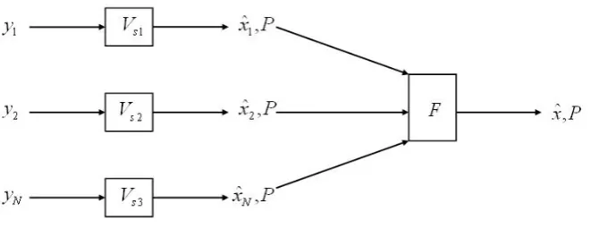
Suppose there is N sensor at same sampling rate. Because we allow sensor to measure synchronously, the measurement is assumed to come at the same number during a period, where the time distance between two measurements is uniform. For every measurement coming from these sensors that is received in fusion center, there is a corresponding estimation based solely on one sensor that is taken in so called the virtual sensor (VS). Suppose at VS, the last estimate update is attkand the next estimate time istk+1=tki+Tsi,

where Tsi is constant sampling time for all corresponding VS. Every estimation from single VS then is

processed through the fusion algorithm to get optimal estimation of the state. Overall diagram of fusion pro-cess using multiple sensors can be seen in Fig. 1. When estimate of different states are available, based on theira–prioriknowledge, the problem now turns how to combine these different estimations to get the optimal result. Fused estimation based on the series of particular sensors are computed every sampling time

Ts, where the fused estimationβˆ(k|k)is no more than an estimation coming from each sensorxˆi(k|k)(See

(16)

Theorem 5.1 For anyk = 1,2,3.... the estimate and the estimation error covariance ofβ(k)based on all

the observations before timekTare denoted byβˆ(k|k)andP(k|k)respectively, then they can be generated

by the use of the following formula:

ˆ

β(k|k) =

N ∑

i=1

βi(k) ˆβN|i(k|k) (5.1)

P(k|k) = (

N ∑

i=1

P_N−_|1_i(k|k))−1 (5.2)

where,

βi(k) = P(k|k)P_N−_|1_i(k|k) (5.3)

whereβˆN|i(k|k)is state estimation at the highest sample rate based on estimation from VSiandPN|i(k|k) is it’s error covariance.

The fused estimationβˆ(k|k)is no more than a weighted estimation coming from each sensorβˆi(k|k).

In-tuitively, one can think that the estimation from sensori, that has less error covariance should be weighted

more, compared to those that has higher error covariance e.g. if we have N number of faulty sensors,

then the VS with less fault will have less error covariance, and therefore it should be weighted more and

vice versa. Moreover, following the procedure of selection of state estimations (from their weighted

corre-sponding VS), we will get the optimal result in sense of error variance with the assumption that there is no

cross-covariance among VS’s estimations.

From equation (5.3), it can be verified that:

P(k|k)≤PN|i(k|k) (5.4)

which means that the fused estimation error from estimation of different sensors are always be less or equal

to the estimation error of each sensor.

6 Evaluation and Testing

(17)

6.1 Experimental Setup and Process Data Collection

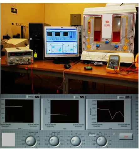
The data for the bench-marked laboratory-scale two-tank process control system has been collected at a sampling rate of50milliseconds. Process data has been generated through an experimental setup as shown in Fig. 2. The prime objective of the bench-marked dual-tank system is to reach a reference height of200 ml of the second tank. During this process, several faults have been introduced such as the leakage faults, sensor faults and actuator faults. Leakage faults have been introduced through the pipe clogs of the system, knobs between the first and the second tank etc. Sensor faults have been introduced by introducing a gain in the circuit as if there is a fault in the level sensor of the tank. Actuator faults have been introduced by introducing a gain in the setup for the actuator that comprises of the motor and pump. A Proportional and Integral (PI) controller works in a closed loop configuration to reach the desired height of the second tank. Due to the inclusion of faults, the controller was finding it difficult to reach the desired level. For this rea-son, the power of the motor has been increased from a scale of0to5volts to scale of5to18volts in order to provide it the maximum throttle to reach the desired level. In doing so, the actuator performed well in achieving its desired level but it also suppressed the faults of the system. So, it made the task of detecting the faults even more difficult. After the collection of data, techniques such as settling time, steady state value, and coherence spectra can help us to give an insight of the fault.

In this paper, in particular, leakage fault has been considered. Hydraulic height and liquid output flow-rate of the second tank are the inputs while leakage fault level on a discrete scale of1to4is the considered output. Data is collected by introducing leakage fault in the closed loop system.

6.2 Model of the Coupled Tank System

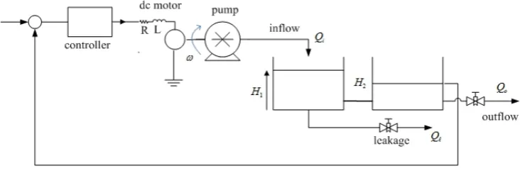
The physical system under evaluation is formed of two tanks connected by a pipe. The leakage is simulated in the tank by opening the drain valve. A DC motor-driven pump supplies the fluid to the first tank and a PI controller is used to control the fluid level in the second tank by maintaining the level at a specified level, as shown in Fig. 3.

(18)

Figure 2: A – The two tank system interfaced with the Labview through a DAQ and the amplifier for the magnified voltage , B – The labview setup of the apparatus including the circuit window and the block diagram of the experiment.

faults are introduced and the liquid height in the second tankH2, and the inflow rateQi, are both measured.

The National Instruments Labview package is employed to collect these data.

A benchmark model of a cascade connection of a DC motor and a pump relating the input to the motoru

and the flowQiis a first-order system:

˙

Qi =−amQi+bmϕ(u) (6.1)

whereamandbmare the parameters of the motor-pump system,ϕ(u)is a dead-band and saturation type

of nonlinearity andQ˙iis the rate of change of input flow. It is assumed that the leakageQℓoccurs in tank1

and is given by:

Qℓ=Cda √

2gH1 (6.2)

whereCda is the discharge coefficient of the leakage valve in tank1,H1 is the liquid height in the first

tank andg= 980cm/sec2 is the gravitational constant. With the inclusion of the leakage, the liquid level system is modeled by (See equation (6.3)):

A1

dH1

dt =Qi−Cdbφ(H1−H2)−Cdaφ(H1) (6.3) A2

dH2

(19)

whereφ(.) =sign(.)√2g(.),Qℓ=Cdaφ(H1)is the leakage flow rate,Q0 =Cdcφ(H2)is the output

flow rate,A1andA2are the cross-sectional areas of the two tanks,CdbandCdcare the discharge coefficient

of the leakage valve in tank2and output valves respectively.

The model of the two-tank fluid control system, shown in Fig. 3, is of a second order and is nonlinear with a smooth square-root type of nonlinearity. For design purposes, a linearized model of the fluid system is required and is given below in (6.5) and (6.6):

dh1

dt =b1qi−(a1+γ)h1+a1h2 (6.5) dh2

dt =a2h1−(a2−β)h2 (6.6)

where h1 andh2 are the increments in the nominal (leakage-free) to heights H10 and H20. Parameters

γ and β indicate the amount of leakage and output flow rate respectively, where γ = Cda

2√2gH0 1

andβ =

Cdc

2√2gH0 2

. Alsob1 =_A1₁,a1= Cdb 2√2g(H0

1−H20)

anda2 =a1+ Cdc 2√2gH0

2 .

A PI controller, with gainskp andkI, is used to maintain the level of the tank2at the desired reference

inputras:

˙

x3 =e=r−h2

u=kpe+kIx3

(6.7)

wherex˙3is the rate of change of error,ris the reference height of tank2.i.e. 200 ml andh2is the height

of the tank2achieved anduis the control input. The linearized model of the entire system formed by the motor, pump, and the tanks is given by:

˙

x=Ax+Br y=Cx (6.8)

where x=           h1 h2 x3 qi          

, A=

         

−a1−γ a1 0 b1

a2 −a2−β 0 0

−1 0 0 0

−bmkp 0 bmkI −am

          , B= [

0 0 1 b k

]T

, C = [1 0 0 0]

(20)

Figure 3: Process control system: A Lab-scale two-tank system

Here qi,qℓ,q0,h1 andh2 are the increments in Qi,Qℓ, Q0,H10 andH20 respectively. The parameters

a1anda2 are associated with linearization. As the parametersγ andβ are respectively associated with the

leakage and the output flow rate, so they presentqℓ=γh1 andq0=βh2.

Remark 6.1 During the implementation process,sign(.) can be approximated witharc tangent. A

rela-tionship for approximation can be expressed as follows:

sign(x) = arctan(√ x

1−x∗x), where x <1 (6.10)

6.3 Evaluation Results

(21)

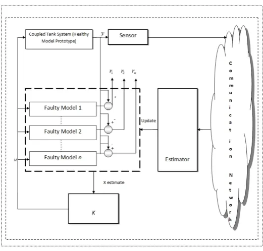
con-Figure 4: Architecture of Coupled Tank system in distributed control network

trol system. For each test case, we will run the modified Bayesian-based KF and the standard Bayesian-KF and show their comparisons for various cases, moreover compute the time computation of state estimates and show the results in Table 1 and 2 respectively.

Remark 6.2 It should be noted here that height sensor as shown in Fig. 2 interface diagram with labview

is being used in the coupled tank system for the purpose of data fusion. Moreover, the potency of the leakage

fault i.e small, medium or large is being defined with the help of the leakage knobs facility between the two

tank tanks and drainage as shown in the main diagram of Fig. 2.

6.3.1 Leakage Fault: Estimates and Covariance Comparison with Complete and Incompleteprior

information cases

The Bayesian-based FB KF has been simulated here for the leakage fault of the plant. Simulations have been made for the x-estimate and the covariance of each case. In the simulation, comparisons of various levels of leakage i.e. no, small, and medium intensity of leakage faults, and distributed estimation have been shown.

(22)

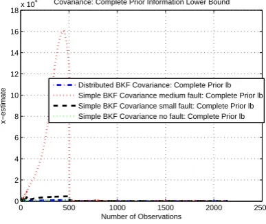
Fig. 6) that the distributed structure is clearly performing well as compared to the other profiles. When it comes to the covariance and estimate of modified filter implementation with ub (see Fig. 7 for covariance of ub scheme and see Fig. 8 for estimate of ub scheme) and lb (see Fig. 9 for covariance of lb scheme and see Fig. 10 for estimate of lb scheme), it is performing equally well for distributed structure. The advantage of using the modified upper and lb filters can be seen more clearly in the time computation comparison and mean square error (MSE) as discussed in the next Section.

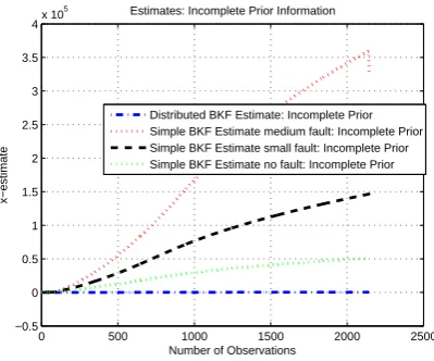
For incomplete prior information, it can be seen for the estimate profile (see Fig. 11) that the distributed structure is clearly performing well as compared to the other profiles, when it comes to the covariance and estimate of modified filter implementation with ub (see Fig. 12) for estimate of ub scheme and lb, it is performing equally well for distributed structure. Moreover, other estimates shown in Fig. 13 also elaborate the performance of distributed estimation and estimation of the modified filters.1

6.4 Time Computation and MSE

In this section, we have discussed the time computation and MSE of different methods which have been employed for calculating the estimates and covariances of the state with complete prior information, and incomplete prior information. An equal number of5iterations have been run for achieving each and every of the estimate.

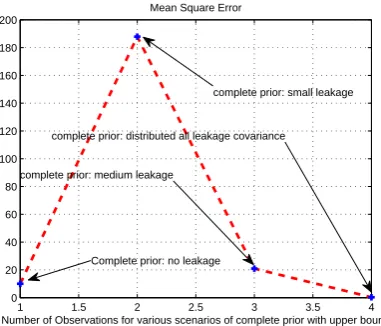
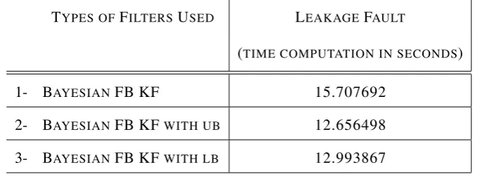
For the case of complete prior information, it can be seen from Table 1, that iteration time of the basic Bayesian-based FB KF, though it is very much optimal in nature due to its structure than the regular KF, is taking the maximum number of time for the computation, whereas both modified filters of ub and lb are performing well in time computation for the leakage fault. More precisely, the performance of distributed version and lb and ub can be seen in Fig. 14-16, where the performance of distributed version and modified filters is quiet visible.

Likewise is the case of incomplete prior information (See Table 2) which is even more crucial and critical because of the structure, and here the basic Bayesian-based FB KF is taking comparatively more time than 1_{Fig. 5-13 shows the comparison of estimates and covariance for types of}_a₋_priori_{information cases. In all these figures}

x-axis shows the number of observations taken at a sampling rate of50milliseconds of time, andy-axis shows the X-estimate which

(23)

0 500 1000 1500 2000 2500 0

2000 4000 6000 8000 10000 12000

Number of Observations

x−estimate

Covariance: Complete Prior Information

Distributed BKF Covariance: Complete Prior Simple BKF Covariance medium fault: Complete Prior Simple BKF Covariance small fault: Complete Prior Simple BKF Covariance no fault: Complete Prior

Figure 5: Comparison of Covariance for complete prior information for Leakage Fault

0 500 1000 1500 2000 2500

−0.5 0 0.5 1 1.5 2 2.5 3 3.5x 10

4

x−estimate

Estimates: Complete Prior Information

Distributed BKF Estimate: Complete Prior Simple BKF Estimate medium fault: Complete Prior Simple BKF Estimate small fault: Complete Prior Simple BKF Estimate no fault: Complete Prior

Figure 6: Comparison of Estimates for complete prior information for Leakage Fault

0 500 1000 1500 2000 2500

−6 −4 −2 0 2 4 6x 10

9

x−estimate

Covariance: Complete Prior Information Upper Bound

Distributed BKF Covariance: Complete Prior ub Simple BKF Covariance medium fault: Complete Prior ub Simple BKF Covariance small fault: Complete Prior ub Simple BKF Covariance no fault: Complete Prior ub

(24)

0 500 1000 1500 2000 2500 −3 −2 −1 0 1 2 3 4 5 6x 10

4

x−estimate

Estimates: Complete Prior Information Upper Bound

Distributed BKF Estimate: Complete Prior ub Simple BKF Estimate medium fault: Complete Prior ub Simple BKF Estimate small fault: Complete Prior ub Simple BKF Estimate no fault: Complete Prior ub

Figure 8: Comparison of Estimates for complete prior information for Leakage Fault with ub Modified Filter

0 500 1000 1500 2000 2500

0 2 4 6 8 10 12 14 16 18x 10

4

x−estimate

Covariance: Complete Prior Information Lower Bound

Distributed BKF Covariance: Complete Prior lb Simple BKF Covariance medium fault: Complete Prior lb Simple BKF Covariance small fault: Complete Prior lb Simple BKF Covariance no fault: Complete Prior lb

Figure 9: Comparison of Covariance for complete prior information for Leakage Fault with lb Modified Filter

0 500 1000 1500 2000 2500

0 0.5 1 1.5 2 2.5

3x 10

4

x−estimate

Estimates: Complete Prior Information Loweer Bound

Distributed BKF Estimate: Complete Prior lb Simple BKF Estimate medium fault: Complete Prior lb Simple BKF Estimate small fault: Complete Prior lb Simple BKF Estimate no fault: Complete Prior lb

(25)

0 500 1000 1500 2000 2500 −0.5

0 0.5 1 1.5 2 2.5 3 3.5

4x 10

5

x−estimate

Estimates: Incomplete Prior Information

Distributed BKF Estimate: Incomplete Prior Simple BKF Estimate medium fault: Incomplete Prior Simple BKF Estimate small fault: Incomplete Prior Simple BKF Estimate no fault: Incomplete Prior

Figure 11: Comparison of Estimates for Incomplete prior information for Leakage Fault

0 500 1000 1500 2000 2500

−2500 −2000 −1500 −1000 −500 0 500 1000

x−estimate

Estimates: Incomplete Prior Information with Upper Bound

Distributed BKF Estimate: Incomplete Prior Simple BKF Estimate medium leak: Incomplete Prior Simple BKF Estimate small leak: Incomplete Prior Simple BKF Estimate no leak: Incomplete Prior

Figure 12: Comparison of Estimates for Incomplete prior information for Leakage Fault

0 500 1000 1500 2000 2500

−1500 −1000 −500 0 500 1000

x−estimate

Estimate 2: Estimates of Incomplete Prior Information

Distributed BKF Estimate: Incomplete Prior Simple BKF Estimate: Incomplete Prior Sensor 2: Small Leak Height Profile

(26)

1 1.5 2 2.5 3 3.5 4 1

2 3 4 5 6 7 8

X: 4 Y: 1.065

Number of Observtions: Comparison of 4 cases of Prior Knowledge Mean Square Error

Complete Prior: Covariance small fault

Complete Prior: Covariance medium fault

Complete Prior: Covariance no fault

Complete Prior: Distributed Covariance

Figure 14: MSE for Complete Prior Case

1 1.5 2 2.5 3 3.5 4

0 1 2 3 4 5 6

Number of Observations for various cases of Complete Prior lower bound Mean Square Error

Complete Prior lb: no leak

Complete Prior lb: small leak

Complete Prior lb: medium leak

Complete Prior lb: Distributed all leak covariance

Figure 15: MSE for Complete Prior Case with lb

1 1.5 2 2.5 3 3.5 4

0 20 40 60 80 100 120 140 160 180 200

Number of Observations for various scenarios of complete prior with upper bound Mean Square Error

Complete prior: no leakage

complete prior: small leakage

complete prior: medium leakage

complete prior: distributed all leakage covariance

(27)

Table 1: Case I: Time Computation Comparison for Complete Prior Information TYPES OFFILTERSUSED LEAKAGEFAULT

(TIME COMPUTATION IN SECONDS)

1- BAYESIANFB KF 15.707692

2- BAYESIANFB KF WITH UB 12.656498 3- BAYESIANFB KF WITH LB 12.993867

Table 2: Case II: Time Computation Comparison for Incomplete Prior Information TYPES OFFILTERSUSED LEAKAGEFAULT

(TIME COMPUTATION IN SECONDS)

1- BAYESIANFB KF 13.451193

2- BAYESIANFB KF WITH UB 12.996375 3- BAYESIANFB KF WITH LB 11.915037

the likes of modified lb and ub filters. The performance of the modified filters was consistent even here for the leakage fault.

7 Conclusions

(28)

Acknowledgments

The authors would like to thank the deanship for scientific research (DSR) at KFUPM for support through research group projectRG1105-1.

Appendix

A. Proof of Theorem 3.1 For linear estimation ofαusing dataΥwith linear modelΥ =C0kα+ν, the

prior information consists ofα¯andν¯, andCα=cov(α),Cv=cov(v), andCαv=cov(α, v). When we talk

about prior information, we mean prior information aboutα, that isα¯,Cα, andCα,v.

For the dynamic case, as in KF,

ˆ

α_k/k = ET[αk|Υk] = [ ¯αk|Υk]

= α¯k+CαkΥkC

+ Υk(Υ

k₋_Υ_¯k₎_, _α_¯

k =E[αk]

P_k/k = MSE( ˆα_k/k) =△E[(αk−αˆk/k)(αk−αˆk/k)T]

= Cαk−CαkΥkC

+ ΥkC

T αkΥk

whereC_Υ+is the Moore-Penrose pseudo-inverse ofCΥ, which equalsC_Υ−1wheneverC_Υ−1exists. With few

exceptions, however, it is unrealistic since its computational burden increases rapidly with time (method for decreasing time computation complexity is applied in the next section using modified KF functions of ub and lb.

ˆ

αk/k = ET[αk|yk] =ET[αk|yk, yk−1] = ˆαk/k−1+Kky¯k/k−1

Pk/k = MSE( ˆαk/k) =MSE( ˆαk/k−1)−KkCΥ¯k/k−1KkT

whereα˜k|k−1=αk-αˆk|k−1,Kk=Cα˜k|k−1Υ˜k|k−1C

+ ˜

αk|k−1, ˜

(29)

LetA=Pk/kandΦk=ζ. Equation (3.12) follows from the following:

(ζP C₀T_k+A)(C+C0kA)−

1

= {ζ[Cα−(CαC0Tk+A)(C0kCαC

T

0k+C+C0kA+ (C0kA)

T₎−1

. (CxC0Tk +A)

T_]_CT

0k+A}(C+C0kA)−

1

= (ζCα+C0Tk+A)[I−(C0kCxC

T

0k+C+C0kA+ (C0kA)

T₎−1

. (HCαC0Tk + (C0kA)

T_)](_C₊_C

0kA)−

1

= (ζCαC0Tk+A)(C0kCαC

T

0k+C+C0kA+ (C0kA)

T₎−1

. (C+C0kA)(C+C0kA)−

1

= (ζCαC0Tk+A)(CΥ+C0kA)

−1

B. Proof of lemma 3.1 Using (3.16), we have

P(k+ 1|k)−P(k+ 1|k) = E[Θ(Z)P(k|k)Θ(Z)T]

+ E[Θ(Z)αb(k|k)αb(k|k)TΘ(Z)T]

− Θbαb(k|k)αb(k|k)TΘbT −ΘbP(k|k)ΘbT

− K_p,kR_e,kK_p,k+Kp,kRe,kKp,k

= P1+P2 (7.1)

whereP1=E[Θ(Z)P(k|k)Θ(Z)T]−ΘbP(k|k)AbT−Kp,kRe,kKp,kandP2=E[Θ(Z)αb(k|k)αb(k|k)TΘ(Z)T]−

b

Θαb(k|k)αb(k|k)T_ΘbT ₊_K

p,kRe,kKp,k.

IfP1≥0andP2≥0, thenP(k+ 1|k)−P(k+ 1|k)≥0

P1 = E[Θ(Z)P(k|k)Θ(Z)T]−ΘbP(k|k)ΘbT −Kp,kRe,kKTp,k

− ΘbP(k|k)ΘbT +ΘbP(k|k)ΘbT

= E[Θ(Z)P(k|k)Θ(Z)T]−ΘbP(k|k)ΘbT

+ Θ(b P(k|k)−P(k|k))ΘbT −K_p,kR_e,kKT_p,k (7.2)

(30)

unitary matrix andD1is a diagonal matrix. Hence,

P1 = E[(Θ(Z)U1D11/2)(Θ(Z)U1D11/2)T]

− E[(Θ(Z)U1D11/2)]E[(Θ(Z)U1D11/2)]T

+ Θ(b P(k|k)−P(k|k))ΘbT −K_p,kR_e,kKT_p,k

= Cov[(Θ(Z)U1D11/2] +Θ(b P(k|k)−P(k|k))ΘbT

− K_p,kR_e,kK_p,k (7.3)

whereCov[C0k]denotes the covariance matrix ofC0k. Since a covariance matrix is positive definite and

P(k|k)−P(k|k)≥0by assumption,P1≥0.P2is a covariance matrix sinceαb(k|k)αb(k|k)T is symmetric,

henceP2≥0.

C. Proof of lemma 3.2 Here, we will use matrix inversion lemma which says that(A+U CV)−1 =

A−1 −A−1U(C−1 +V A−1U)−1V A−1 where A, U, C and V all denote matrices of the correct size. Applying the matrix inversion lemma to (3.18), we haveP(k+ 1|k+ 1) = (P(k+ 1|k)−1+C₀T

kR

−1_C 0k)−

1_.

LetP =P(k+ 1|k)andP =P(k+ 1|k). ThenP ≥P⇒P−1 _≤_P−1_{. Also,}_P₋1₊_CT

0kR

−1_C

0k≤P−

1

+C₀T

kR

−1_C_⇒₍_P−1₊_CT

0kR

−1_C 0k)−

1_≥₍_P−1₊_CT

0kR

−1_C 0k)−

1_{. Thus,}

P(k+ 1|k+ 1) ≥ P(k+ 1|k+ 1) (7.4)

D. Proof of lemma 3.3 LetM =αb(k|k)αb(k|k)T andI be an identity matrix. Then using (3.16), we have

P(k|k)−P(k|k) = λmaxE[Θ(Z)Θ(Z)T]

− E[Θ(Z)P(k|k)Θ(Z)T]−E[Θ(Z)MΘ(Z)T]

− KpRe,kKpT +KpRe,kK

T p

= E[Θ(Z)(λmax(P(k|k))I−P(k|k))Θ(Z)T]

+ E[Θ(Z)(λmax(M)I −M)Θ(Z)T]

− KpRe,kKpT +KpRe,kK

T

p (7.5)

(31)

E. Proof of theorem 3.4 Let us consider the lb-KF. LetP_k =P_k_|_k. ψ=GQGT,Θ =ˆ E[Θ], andΦ =

−(C0kΘˆPkΘˆ

T_CT

0k+C0kψC

T

0k +R)

−1₍_C

0kψ+CAPˆ kΘˆ

T_).

Then based on Riccati difference equation [29], we can expressP_k₊₁as:

P_k₊₁ = ΘˆP_kΘˆT +ψ

− ΦT(C0kΘˆPkΘˆ

T_CT

0k +C0kψC

T

0k+R)F

= ( ˆΘT + ˆΘTC₀T_kF)TP_k( ˆΘT + ˆΘTC₀T_kΦ)

+ ΦT(C0kψC

T

0k+R)Φ +ψC

T

0kΦ + Φ

T_C

0kψ+ψ (7.6)

Hence, if( ˆΘT _{+ ˆ}_ΘT_CT

0kΦ)is not a stability matrix, for someP0≤P(0|0). Pkdiverges ask→ ∞. Since

the state error covariance of the lb-KF diverges andP(k|k)≤P(k|k)for allk≥0(Theorem 3.2),P(k|k) diverges as k → ∞. Here P(k|k) can be ΦkPk+1/kΦTk −KkC0kPk+1/k for ‘complete’ prior case and

KkC0kPk/k−1for ‘incomplete’ prior case respectively.

F. Proof of theorem 4.1 By explanation ofB, the problem can be considered for incomplete prior infor-mation withC0k andCreplaced by theC˜0k andC˜ respectively, where, from the proof of Theorem 4.1, the

estimate isu=VTx, whereV is an orthogonal matrix. This means that Theorem 4.1 is applicable now to

u. Therefore:

b

α = Vu, Pˆ = VMSE(ˆu)VT

The uniqueness result thus follows from Theorem 4.1.

G. Proof of lemma 4.1 Using (4.11), we have

P(k+ 1|k)−P(k+ 1|k) = E[Θ(Z)αb(k|k)αb(k|k)TΘ(Z)T]

− Kp,kRe,kKp,kT

− Θbαb(k|k)αb(k|k)TΘbT

+ K_p,kR_e,kKT_p,k

= P1+P2 (7.7)

(32)

SinceP(k|k)is a symmetric matrix,P(k|k)can be decomposed intoP(k|k)=U1D1U1T, whereU1is a

unitary matrix andD1is a diagonal matrix, but here there is noP(k|k)forP1.

H. Proof of lemma 4.2 LetM =αb(k|k)αb(k|k)T andIbe an identity matrix. Then using (4.11), we have

P(k|k)−P(k|k) = E[Θ(Z)(λmax(M)I−M)Θ(Z)T]

+ ΘˆMΘˆT +Kp,kRe,kK T p,k

− Kp,kRe,kKp,kT

+ GQGT (7.8)

Since,P(k|k)≥P(k|k)andλmax(S)I−S≥0for any symmetric matrixS,P(k|k)−P(k|k)≥0.

References

[1] Rao, B. S., and Whyte, H. F., ‘Fully decentralised algorithm for multisensor Kalman filtering’,IEEE Proceedings-D Control Theory and Applications, vol. 138(5), pp. 413–420, September 1991.

[2] Chong, C. Y., Chang, K. C., Mori, S., ‘Distributed tracking in distributed sensor networks’,American Control Conference, pp. 1863–1868, Seattle, 18-20 June 1986.

[3] Hashmipour, H. R., Roy, S., Laub, A. J., ‘Decentralized structures for parallel Kalman filtering’,IEEE Trans. on Autom. Control, vol. 33(1), pp. 88–94, 1988.

[4] Luo, Y., Zhu, Y., Luo, D., Zhou, J., Song, E., and Wang, D., ‘Globally optimal multisensor distributed random parameter matrices Kalman filtering fusion with applications’,Sensors 2008, vol. 8(12), pp. 8086–8103, 2008.

[5] Schizas, D. I., Giannakis, G. B., and Luo, Z. Q., ‘Distributed estimation using reduced-dimensionality sensor observations’, IEEE Trans. Signal Processing, vol. 55(8), pp. 4285–4299, 2007.

(33)

[7] Bar-Shalom, Y., editor, ‘Multi-target-multi-sensor tracking: advanced applications’,Atech House, Nor-wood, MA, vol. 1, 1990.

[8] Hashmipour, H. R., Roy, S., and Laub, A. J., ‘Decentralized structures for parallel Kalman filtering’,

IEEE Trans. Automatic Control, vol. 33(1), pp. 88–93, 1988.

[9] Chong, C. Y., Mori, S., and Chang, K. C., ‘Distributed multi-target multi-sensor tracking’, In Multitarget-Multisensor Tracking: Advanced Applications (Bar-Shalom, ed.), vol. 1, Atech House, Norwood, MA, 1990.

[10] Liggins, M., Chong, C. Y., Kadar I., Alford, M. G., Vannicola, V., and Thomopoulos, S., ‘Distributed fusion architectures and algorithms for target tracking’,Proc. the IEEE, vol. 85(1), pp. 95–107, 1997. [11] Saber, R. O., and Murray, R. M., ‘Consensus problems in networks of agents with switching topology

and time-delays’,IEEE Trans. on Automatic Control, vol. 49(9), pp. 1520-1533, Sep. 2004.

[12] Mesbahi, M., ‘On state-dependent dynamic graphs and their controllability properties’,IEEE Trans. on Automatic Control, vol. 50(3), pp. 387-392, 2005.

[13] Moreau, L., ‘Stability of multiagent systems with time-dependent communication links’,IEEE Trans. on Automatic Control, vol. 50(2), pp. 169-182, 2005.

[14] Ren, W., and Beard, R. W., ‘Consensus seeking in multi-agent systems under dynamically changing interaction topologies’,IEEE Trans. on Automatic Control, vol. 50(5), pp. 655-661, 2005.

[15] Xiao, L., and Boyd, S., ‘Fast linear iterations for distributed averaging’,Systems and Control Letters, vol. 52, pp. 65-78, 2004.

[16] Saber, O. R., ‘Flocking for multi-agent dynamic systems: Algorithms and theory’,IEEE Transactions on Automatic Control, vol. 51(3), pp. 401-420, March 2006.

[17] Yang, X., ’Particle swarm optimisation particle filtering for dual estimation’, IET Signal Processing, vol. 6(2), pp. 114–121, April 2012.

(34)

[19] Grimble, M. J., and Naz, S. A., ’Optimal minimum variance estimation for non-linear discrete-time multichannel systems’,IET Signal Processing, vol. 4(6), pp. 618–629, December 2010.

[20] Grimble, M. J., ’Non-linear minimum variance state-space-based estimation for discrete-time multi-channel systems’,IET Signal Processing, vol. 5(4), pp. 365–378, July 2011.

[21] Xu, J., and Li, J. X., ’State estimation with quantised sensor information in wireless sensor networks’,

IET Signal Processing, Febraury, 2011, vol. 5(1), pp. 16–26.

[22] Al-Naffouri, T. Y., ’An EM-based forward backward Kalman filter for the estimation of time-variant channels in OFDM’,IEEE Transactions on Signal Processing, vol. 1(11), pp. 1–7, November 2006.

[23] Mahmoud, M. S., and Khalid, H. M., ’Expectation maximization approach to data-based fault diag-nostics’,Special Issue: Information Sciences, Elsevier, DOI: S002002551200059X, 2012.

[24] Oh, S., and Sastry, S., ‘Approximate estimation of distributed networked control system’, 2007 ACC ’07 American Control Conference, pp. 997–1002, 9-13 July 2007.

[25] Chen, Z., ‘Bayesian filtering: From Kalman filters to particle filters and beyond’,adaptive Syst Lab McMaster Univ Hamilton ON Canada, Citeseer, , pp. 9–13, 25–46, 2003.

[26] Li, R., X., Zhu, Y., Wang, J., and Han, C., ‘Optimal linear estimation fusionpart I: unified fusion Rules’,IEEE Transactions on Information Theory, vol. 49(9), pp. 2192–2208, September 2003.

[27] Mahmoud, M. S., and Emzir, M. F., ‘State estimation with asynchronous multi-rate multi-smart sen-sors’,Information Sciences, volume 196(1), pp. 15-27, August 2012.

[28] Doraiswami, R., Cheded, L., and Khalid, H. M.,. ’Model order selection criterion with application to physical systems’,6th IEEE Conference on Automation, Science and Engineering (CASE), pp. 393 – 398, Toronto, Canada, August 21–24, 2010.