Improved Simultaneous Estimation of Location and System Reliability via Shrinkage Ideas

(1)

University of South Carolina

Scholar Commons

Theses and Dissertations

2017

Computational Wave Field Modeling using

Sequential Mapping of Poly-Crepitus Green’s

Function in Anisotropic Media

Sajan Shrestha

University of South Carolina - Columbia

Follow this and additional works at:https://scholarcommons.sc.edu/etd Part of theMechanical Engineering Commons

This Open Access Dissertation is brought to you by Scholar Commons. It has been accepted for inclusion in Theses and Dissertations by an authorized administrator of Scholar Commons. For more information, please [email protected].

Recommended Citation

Shrestha, S.(2017).Computational Wave Field Modeling using Sequential Mapping of Poly-Crepitus Green’s Function in Anisotropic Media.

(2)

COMPUTATIONAL

WAVE

FIELD

MODELING

USING

SEQUENTIAL

MAPPING

OF

POLY-CREPITUS

GREEN’S

FUNCTION

IN

ANISOTROPIC

MEDIA

by Sajan Shrestha

Bachelor of Science Benedict College, 2014

Submitted in Partial Fulfillment of the Requirements For the Degree of Master of Science in

Mechanical Engineering

College of Engineering and Computing University of South Carolina

2017

Accepted by:

Sourav Banerjee, Director of Thesis Victor Giurgiutiu, Reader

(3)

(4)

DEDICATION

(5)

ACKNOWLEDGEMENTS

(6)

ABSTRACT

(7)

(8)

LIST OF FIGURES

Figure 4.1 An artistic view showing the schematics of the wave field inside a bulk

anisotropic media ...13

Figure 4.2 a) Schematics of the wave surfaces and their relation b) relation of the phase velocity with the fundamental wave modes in anisotropic media. ...16

Figure 4.3 Pictorial representation of the Christoffel’s solution...20

Figure 4.4 For Aluminum: 3D Slowness plot, Y Contour plot, Y-Z Contour plot, and X-Z Contour plot of qL, qS1, qS2 modes ...25

Figure 4.5 For Transversely Isotropic: 3D Slowness plot, X-Y Contour plot, Y-Z Contour plot, and X-Z Contour plot of qL, qS1, qS2 modes ...26

Figure 4.6 For Orthotropic: 3D Slowness plot, X-Y Contour plot, Y-Z Contour plot, and X-Z Contour plot of qL, qS1, qS2 modes ...27

Figure 4.7 For Monoclinic: 3D Slowness plot, X-Y Contour plot, Y-Z Contour plot, and X-Z Contour plot of qL, qS1, qS2 modes ...28

Figure 4.8 A schematic diagram to visualize the Radon transform in 2D and 3D ...31

Figure 4.9 A schematic diagram to visualize the displacement Green’s function ...36

Figure 5.1 Schematics of configurations to calculate the Green’s function ...39

Figure 5.2 Numerical computation of displacement Green’s function due to forces acting along 1, 2 & 3directions when the inside material is Isotropic. ...39

Figure 5.3 Numerical computation of displacement Green’s function due to forces acting along 1, 2 & 3directions when the inside material is Transversely Isotropic. ...40

Figure 5.4 Numerical computation of displacement Green’s function due to forces acting along 1, 2 & 3directions when the inside material is Orthotropic. ...40

(10)

Figure 5.6 Numerical computation of displacement Green’s function (unit mm) in Transversely Isotropic material...42 Figure 5.7 Numerical computation of Stress Green’s function in Transversely Isotropic material due to source actuating along 1-direction ...43 Figure 5.8 Numerical computation of Stress Green’s function in Transversely Isotropic material due to source actuating along 3-direction ...43 Figure 6.1 a) the total field at A is calculated by superposing the contribution of all point sources distributed along the boundary of the anisotropic medium. b) the three mutually perpendicular forces that are contained in the point source ...45 Figure 6.2 a) Schematics (not to scale) of the wave field computation problem in anisotropic solid half space, point sources distributed over the x-y plane, however, only two orthogonal line of point sources are shown b) cross-section view of the NDE problem along x-z plane. ...46 Figure 6.3 A schematics showing the sequential mapping of Green’s function, a) source and target point combinations b) extended target points in 2D c) Calculated Green’s function on extended point sources d) Assignment of Green’s function for an edge source e) source-target combinations in 3D, f) sequential mapping of 3D Green’s function. ...53

Figure 6.4 a) Convergence study with the discretization angle for Green’s function computation b) Increase in computational efficiency while solving a virtual NDE problem described in Fig. 2 in a transversely isotropic medium.……….54 Figure 6.5 Pressure and normal stress (σ33) distribution at the fluid-solid interface ...55

Figure 6.6 Wavefield plot a) Stress11 (σ11) distribution in transversely isotropic half-space

b) Stress33 (σ33) distribution in transversely isotropic half-space in GPa ...56

Figure 6.7 Wavefield plot a) Stress11 (σ11) distribution in isotropic half-space b) Stress33

(σ33) distribution in isotropic half space in GPa ...56

(11)

LIST OF SYMBOLS

k Vector representing the wave propagation direction CE Velocity of the wave energy

φ Skew Angle CP Phase velocity

N Wave energy propagation direction n Normal to the slowness surface qL Quasi Longitudinal Wave Mode qSS Quasi Shear Slow Wave Mode qS1 Quasi Shear 1 Wave Mode qFS Quasi Shear Fast Wave Mode qS2 Quasi Shear 2 Wave Mode

𝑥𝑖 Components of vectors in the three Cartesian coordinates

𝜎𝑖𝑗 The stress tensor

𝑢_𝑖 Displacement vector at a point in the solid

𝑓_𝑖 Body force per unit volume

𝐶_{𝑖𝑗𝑚𝑙} Constitutive material property matrix

𝜀𝑚𝑙 Strain tensor

A Scalar amplitude of the wave

(12)

ω Monochromatic wave frequency

𝛿_𝑖𝑚 Dirac delta function

𝜌 Density of the material

𝐶_𝑞𝐿 Phase Velocity for quasi longitudinal mode

𝐶_𝑞𝐹𝑆 Phase Velocity for quasi shear fast mode

𝐶_𝑞𝑆𝑆 Phase Velocity for quasi shear slow mode

𝛗𝐋 Eigen vector for quasi longitudinal mode

𝛗_𝐅𝐒 Eigen vector for quasi shear fast mode

𝛗_𝐒𝐒 Eigen vector for quasi shear slow mode

𝐺_𝑚𝑝 Time domain displacement Green’s function

𝐹_𝑝 Force Amplitude

ℱ Fourier transform

𝐺̃𝑚𝑝 Frequency-wavenumber domain displacement Green’s function

𝐋_𝑖𝑚 ℒ2 Hilbert space operator

𝑔_𝑚𝑝 Frequency domain displacement Green’s function

𝐶_𝑖𝑗 Reduced property matrix

𝑅 Radon transform

ℎ Distance from the origin

𝛍̂

⃗⃗ _{Unit Normal to the local orientation of lines} 𝛾𝑧 z-th eigen value

𝑃_𝑖𝑚 Projection matrix of the eigen mode

𝐻_𝑧 Heaviside step function

𝜃 Spherical angle in spherical coordinate system

𝜙 Spherical angle in spherical coordinate system

(13)

LIST OF ABBREVIATIONS

(14)

CHAPTER

1 INTRODUCTION

(15)

out by sensing the propagated energy from a distant location. For this purpose, there is an absolute need to understand the wave propagation behavior in these structures.

Understanding the wave propagation behavior in different types of materials, isotropic and anisotropic, has been a topic of interest and research since past few decades. Although the fluid and isotropic media is more or less saturated field, the critical wave propagation features in anisotropic media are still not fully understood. Due to the widespread application of engineered anisotropic materials, most popularly as composites, in many different areas of science and technology, significantly mechanical and aerospace industries, understanding the wave phenomena in these materials is of great importance. Wave propagation behavior is studied by investigating wave interaction with the material which manifests in the forms of reflection and transmission wave, giving rise to geometric dispersion. These interactions depend on many factors such as the geometric arrangements, mechanical properties, number and nature of the interfacial conditions and the loading conditions (Nayfeh 1995). The mechanical properties vary from the simple case of isotropic materials to the most general anisotropic ones, namely the "triclinic materials".

(16)

2005). Moreover, it is neither feasible nor cost-effective to perform all the possible experiments with various damage scenarios (Mal, Yin et al. 1991, Mouchtachi, El Guerjouma et al. 2004, Moser, Weber et al. 2005, Li, Liu et al. 2013, Marguères and Meraghni 2013) and geometries. Hence, it is not possible to understand the ultrasonic wave interactions in the structure with all possible damages and material degradation with experiments. Consequently, such task can only be possible by correctly understanding the physics of waves propagation in anisotropic media and numerically simulating the behavior of the application of an accurate and efficient technique. The most effective way to do so is by developing a reliable technology capable of virtually simulating any NDE experiments in a systematic and computationally swift manner, i.e., computational NDE or virtual NDE.

(17)

(18)

CHAPTER 2 HISTORICAL BLACKGROUND OF WAVE FIELD MODELING

Studies of the elastic waves propagation in anisotropic media have been of great interest to researchers in the field of NDE. This interest is further intensified by the recent expansion in the use of anisotropic materials in the form of composite materials, super alloys, and crystal structures in the wide variety of applications. However, the inevitability of the necessity of NDE started during the World War II to realize the upsurge in demand for quality assurance of the mechanical systems, machine components and the defense equipment. With the end of the war, the focus of NDE industry shifted from the defense sector to the human infrastructures due to the colossal growth of industrial sectors. Also, the quality assurance of the aerospace systems such as airplanes, satellites, and spaceships became the new agenda for the government agencies.

(19)

the application of plane wave assumption and the plane wave interaction for the structural components.

Moreover, this rising necessity resulted in the mathematical modeling of the ultrasonic wave using Rayleigh-Sommerfeld integral technique. The technique is simply known as the ray tracing method. The ray tracing method simplified the ultrasonic wave problem by representing the waves as rays. The mathematical analysis involves studying the incident waves and providing the reliable and intuitive understanding of the wave energy through the structure. This technique relies on the high-frequency assumption of the ray theory. With the evolution of the technique, it was later known as dynamic ray tracing technique which required the solution of the Eikonal equation (Biondi 1992) and was used in ultrasonic wave field modeling generated by the ultrasonic transducer. Dynamic ray tracing is an improvement over the previously proposed models with a paraxial approximation for the plane wave incidents. Since it is known that the incident wavefronts are neither plane nor spherical in the real experiments using transducers, we had an understanding which was inaccurate, therefore, incomplete. Also, the technique involved significant information loss due to failure to extract exact amplitude information and track all the wave modes in the complex media.

(20)

anisotropic media(Achenbach 1975). Various techniques have been used in the derivation of Green’s function. It has been derived using Cagniard de Hoop method by Kraut (Kraut 1963) for transversely isotropic half-space and by Burridge (Burridge 1971) for an anisotropic halfspace. Simplified method to Cagniard de Hoop has been used by Willis (Willis 1973, Willis 1991) and Payton (Payton 2012) for several anisotropic halfspace problems. The Green’s function for unbounded, anisotropic elastic medium has been developed by Yeatts (Yeatts 1984). Moreover, the method has been further developed by Wang and Achenbach (Wang and Achenbach 1992, Wang and Achenbach 1993) to develop 2-D and 3-D Green’s functions for anisotropic solids.

(21)

(22)

CHAPTER 3 CONCEPTS OF ANISOTROPY

Anisotropic materials have existed in the surrounding environment in nature. Some of the well-known natural anisotropic materials that we see in our daily lives are wood and stones which have been utilized to elevate our standard of living. Hence, due to its usefulness, anisotropic materials are also being engineered most famously as composites. In recent years, manufacturing and usage of composite materials in engineering field has skyrocketed as these materials can be engineered to a required specification. Anisotropic materials such as composites are a combination of two or more materials on a macroscopic scale to form an entirely new useful material. The well-designed composite material has improved properties such as strength stiffness, fatigue life, weight, acoustical insulation and so on.

3.1 Stress-Strain relations for Elastic Materials

The constitutive equation or generalized Hooke’s law relating stresses and strains in anisotropic materials can be formulated in contracted notation as follows,

𝜎_𝑖 = 𝐶_𝑖𝑗𝜀_𝑗

(23)

3.1.1 Stress-Strain relations for Anisotropic Materials

There are materials with the different complexity of anisotropy. Based on the complexity, these materials are categorized as triclinic being fully anisotropic, monoclinic, orthotropic, transversely isotropic and finally, an isotropic material with no anisotropy.

3.1.1.1 Triclinic Materials

The stiffness matrix, 𝐶_𝑖𝑗 has 36 constants. However due to symmetry, there are only 21 independent constants. Therefore, the most general expression of constitutive equation for an elastic material is as follows.

1 11 12 13 14 15 16 1

2 12 22 23 24 25 26 2

3 13 23 33 34 35 36 3

4 14 24 34 44 45 46 4

5 15 25 35 45 55 56 5

6 16 26 36 46 56 66 6

C C C C C C

                                                                        

The above relation characterizes the most general anisotropic material also known as triclinic material. The triclinic material has no planes of material symmetry, and the three material axes are oblique to one another.

3.1.1.2 Monoclinic Materials

(24)

1 11 12 13 16 1

2 12 22 23 26 2

3 13 23 33 36 3

4 44 45 4

5 46 55 5

6 16 26 36 66 6

0 0 0 0 0 0

0 0 0 0

0 0

C C C C

C C

C C C C

                                                                        

The above relation characterizes the anisotropic material known as monoclinic material. The monoclinic material has one plane of material symmetry and has 13 independent elastic constants.

3.1.1.3 Orthotropic Materials

Similarly, if there are two planes of material property symmetry, then there will exist a third mutually orthogonal place with symmetry. Therefore, for the material with three mutually orthogonal planes of symmetry, the constitutive equation reduces to

1 11 12 13 1

2 12 22 23 2

3 13 23 33 3

4 44 4

5 55 5

6 66 6

0 0 0 0 0 0 0 0 0

0 0 0 0 0

C C C

C C C                                                                         

(25)

3.1.1.4 Transversely Isotropic Materials

Now, on top of the three mutually orthogonal planes of symmetry, if there exists a plane of isotropy, i.e., the material properties are same in all directions in that plane (let’s assume 1-2 plane of isotropy), the constitutive equation reduces to

1 11 12 13 1

2 12 11 13 2

3 13 13 33 3

4 44 4

5 44 5

6 11 12 6

0 0 0

0 0 0 0 0

0 0 0 0 0 ( ) / 2

C C C

C C C C                                                           _ _     

The above relation characterizes the anisotropic material known as transversely isotropic material. The transversely isotropic material has five independent elastic constants.

3.1.1.5 Isotropic Materials

Finally, if there exist infinite planes of material property symmetry, i.e., the material property is same in all possible directions, then the constitutive equation reduces to

1 11 12 12 1

2 12 11 12 2

3 12 12 11 3

4 11 12 4

5 11 12 5

6 11 12 6

0 0 0

0 0 0 ( ) / 2 0 0

0 0 0 0 ( ) / 2 0

0 0 0 0 0 ( ) / 2

C C C

C C C C C C                                     _           _             _ _     

(26)

CHAPTER 4 WAVES IN ANISOTROPIC MEDIA

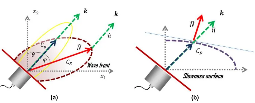
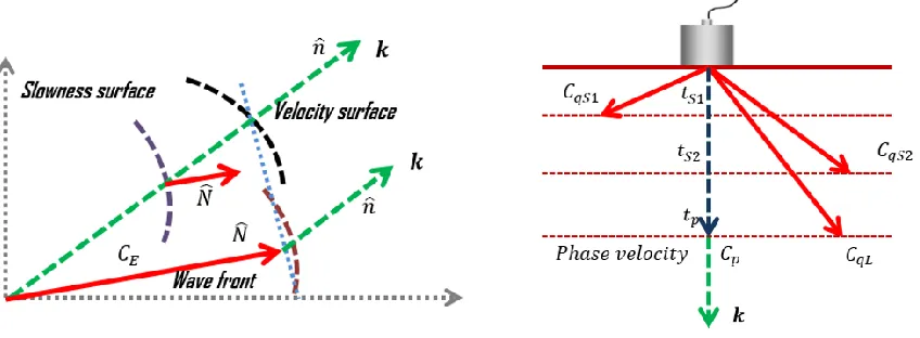
Wave propagation in anisotropic materials is significantly more complicated than in isotropic materials. The anisotropy in a material is caused by various factors such as fine layering, crystal/grain alignment or aligned fractures (Sinclair 2009). The material properties of an isotropic material are independent of the wave propagation direction. However, in an anisotropic material, material properties vary with the direction. Waves in anisotropic media (Auld 1990) does not propagate with spherical wavefront as it is known to exhibit in isotropic materials. Discussing the waves in a fully anisotropic (triclinic) material, let’s assume an ultrasonic transducer attached to an anisotropic media emitting the ultrasonic field in the direction of k vector (Fig. 4.1a).

Fig. 4.1. An artistic view showing the schematics of the wave field inside a bulk anisotropic media a) showing the wavefront b) showing the slowness surface

(27)

If the wave is incident on an isotropic material, the wave energy propagates along the direction of the k vector. However, if the wave is incident on an anisotropic material, the wave does not propagate along k vector. Instead, the wave energy propagates along an entirely different direction creating a new wavefront. The wave propagation in anisotropic media is substantially different to the isotropic case in that elastic waves propagate with a velocity that is dependent on direction. Furthermore, unlike the isotropic case, three fundamental wave modes (Auld 1990, Rokhlin 2011) that propagate can be distinguished into one longitudinal and two shear waves. However, these modes are not necessarily pure modes as the particle vibration, or polarization (Lane 2014). It may be neither parallel nor perpendicular to the propagation direction. Hence, anisotropic modes are referred to as quasi-longitudinal and quasi-shear modes. The quasi-shear modes are further distinguished by their polarization: horizontal or vertical. The wave velocity for each of these modes is direction dependent. The wavefronts of these quasi-modes do not lie normal to the energy propagating direction and hence the phase and wave energy velocities do not coincide. It can be seen in fig 4.1a that the velocity of the wave energy, CE is at an angle φ with respect

to the phase velocity, CP which is in the direction of the wave vector k. Also, the author

(28)

the wave energy propagation is represented by the normal to that slowness surface, i.e., n. Hence the following understanding has been corroborated: in contrast to the phenomena in an isotropic material, the wavefront surfaces and the slowness surfaces are not concentric in the anisotropic material.

(29)

Fig. 4.2. a) Schematics of the wave surfaces and their relation b) relation of the phase velocity with the fundamental wave modes in anisotropic media.

(30)

With the theoretical knowledge gained until now, regarding the wave propagation behavior in anisotropic media, we can see that modeling the anisotropic wave field using the conventional ray tracing methods would be a formidable task. Hence, it can no longer be denied that a simplified and compact mathematical model, incorporating all the behavior mentioned above into the mathematical formulation, is needed for modeling the detailed and exact wave field.

4.1 Visualizing the Modal Wave Velocities

The fundamental elastodynamic equation (eq. 1) in anisotropic material (Auld 1990), which is also known as the equilibrium equation in solid medium, can be written as

𝜎𝑖𝑗,𝑗 + 𝑓𝑖 = 𝜌𝑢̈𝑖 (1)

Where, 𝜎𝑖𝑗 is the stress tensor, 𝑢𝑖 is the displacement vector at a point in the solid,

and 𝑓_𝑖 is the body force per unit volume. From the equation, we can see that the derivative of the stresses is related to the body force and the force due to the dynamic motions, following the Newton’s second law. The stress is related to the strain in a linear elastic media (Rokhlin 2011) through their respective constitutive matrix equation (eq. 2). The material media is assumed linear since the wave has very short exposure time compared to the loading history of the material during the NDE inspection.

𝜎𝑖𝑗 = 𝐶𝑖𝑗𝑚𝑙𝜀𝑚𝑙 (2)

(31)

𝐶_{𝑖𝑗𝑚𝑙} 𝜕2𝑢𝑚

𝜕𝑥𝑗𝜕𝑥𝑙+ 𝑓𝑖 = 𝜌𝑢̈𝑖 (3)

Now, to comprehend the specifics and facts about the phenomena of anisotropic waves, we need to solve this complicated equation. Generally in an NDE experiment, a transducer which has a central actuation frequency is used. It implies that the transducer generates the maximum amplitude of the displacement at that frequency. However, there will be other proximal frequencies generating displacements with gradually lower amplitudes as well. Hence it is challenging, although not impossible, to be able to produce a monochromatic wave actuation with the help of ultrasonic transducer. In agreement to the assumption of linearity of the material, we know that the superposition theorem in the Fourier domain and the reciprocity theorem is valid. Thus, we can proceed to solve the above elastodynamic equation (eq. 3) using a monochromatic harmonic displacement function so that the solution is also valid for nearby frequencies generated by the transducer. Hence, assuming a monochromatic displacement function, we have

𝑢_𝑚 = 𝐴𝑔_𝑚𝑒𝑖(𝐤.𝐱−𝜔𝑡) ₍₄₎

Where, A, is the scalar amplitude of the wave, 𝑔_𝑚is the polarization direction, ω is the monochromatic wave frequency, k is the wave vector, x is the position vector. In addition, k.x represents the dot product between k and x which signifies the phase component of the wave. Subsequent to the assumption of displacement function as above, substituting eq. 4 in to the eq. 3 and simplifying the mathematical expressions (Banerjee and Kundu 2007), we get the following equation eq. 5.

[𝐶_{𝑖𝑗𝑚𝑙}𝑘_𝑗𝑘_𝑙− 𝜌𝛿_𝑖𝑚𝜔2_]𝐴𝑔

(32)

To solve the above equation as an eigenproblem and acquire the eigenvalues and the eigenvectors of a system, we need to consider a homogeneous equation, i.e., the system under the absence of the forcing functions. To do so, we, therefore, proceed to set the body force to zero, i.e., there is no external force acting on the system at the moment. Thus, we beget the nontrivial solution of the equation which can be written as

[𝐶_{𝑖𝑗𝑚𝑙}𝑛_𝑗𝑛_𝑙− 𝜌𝛿_𝑖𝑚𝑐2_]𝑔

𝑚 = 0 (6)

Where, 𝑐2 _{= 𝜔}2_⁄_𝑘2_{is the phase velocity of the wave along the direction of}_k

vector, 𝑛_𝑗 are the direction cosine of the wave propagation direction i.e., along the k vector, and 𝐶𝑖𝑗𝑚𝑙𝑛𝑗𝑛𝑙 is the Christoffel acoustic tensor. By solving the above equation, we are able

to obtain the phase velocities and the phase vectors of the three fundamental wave modes that are propagating in the material with material constants 𝐶_{𝑖𝑗𝑚𝑙}.

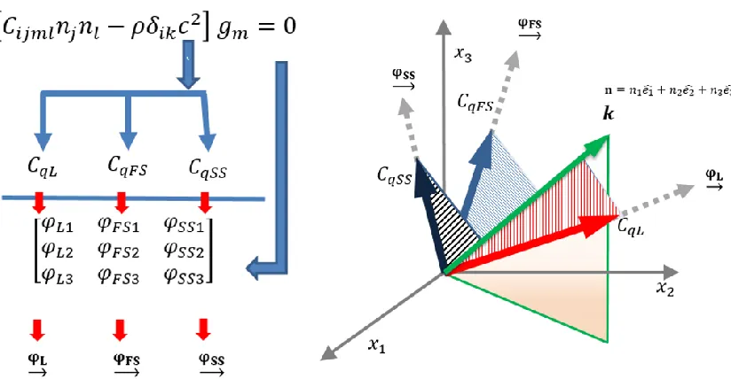
The eq. 6 is well-known as Christoffel’s equation (Christoffel 1877, Auld 1990) which, in our case, defines a set of three homogeneous linear equations for the polarization direction. Each of these equations constitutes an eigenvalue problem with its eigenvalues identified as 𝑐2 along with the accompanying eigen vectors, 𝑔_𝑚. Consequently, the solution of this equation will provide three eigen modes with wave velocities as 𝐶_𝑞𝐿, 𝐶_𝑞𝐹𝑆 and 𝐶_𝑞𝑆𝑆, respectively, along the directions found from the eigen vectors. We are able to enhance our visual understanding with the help of Fig. 4.3. The solution is performed for a specific direction of wave propagation along the k vector with direction normal n. In a 3D coordinate system, the wave velocities are at the direction of their eigen vectors 𝛗_𝐋, 𝛗_𝐅𝐒,

(33)

of the phase velocities. We can clearly see that the summation of projection of the phase velocities of the three wave modes on the k vector gives the resultant phase velocity of the wave along k. However, the wave energy propagation direction is in the direction of the resultant group velocity. In view of the mathematical derivation and understanding that followed in this section, we now are equipped with the tool to compute and determine the modal wave velocities due to wave actuation in any direction just by changing the n vector pointing to any direction in the 3D coordinate system.

Fig. 4.3. Pictorial representation of the Christoffel’s solution where the modal phase wave velocities are the eigenvalues and the direction of those wave modes are the eigenvectors.

4.2 Solution of Elastodynamic Green’s Function

(34)

Green’s function in the anisotropic media (Yeatts 1984, Tverdokhlebov 1988, Kim, Every et al. 1994, Wang 1994, M., Schubert et al. 2000, Every, Pluta et al. 2004). In the upcoming portion of this section, we will see that the vital solution that we acquired by solving the Christoffel’s equation is very crucial in the calculation of the Green’s function.

Now to develop the mathematical formulation of the Green’s function, we revisit the eq. 5. In contrast to transforming the equation into homogeneous in case of Christoffel’s equation, we introduce an impulse force with the help of Dirac Delta function in the media due to a point source, which by definition contributes to the development of the solution of the elastodynamic Green’s function. Based on this development, we modify the equation Eq. 5 to get the Cauchy-Navier Equation as shown below,

[𝐶𝑖𝑗𝑚𝑙 𝜕2

𝜕𝑥𝑗𝜕𝑥𝑙− 𝜌𝛿𝑖𝑚

𝜕2

𝜕𝑡2] 𝐺𝑚𝑝(𝑥𝑛, 𝑡) = −𝛿𝑖𝑝𝛿(𝑥𝒏)𝛿(𝑡)𝐹𝑝 (7)

where, 𝐺_𝑚𝑝(𝑥𝑛, 𝑡) is the time domain Green’s function at 𝑥𝑛 due to a point source

actuation along the m-th direction with force amplitude 𝐹𝑝.

Afterwards, we acquire the governing elastodynamic equation to find the Green’s function at a point 𝑥𝑛 in the frequency-wavenumber domain by transforming the eq. 7 to

the Fourier domain (ℱ) for both spatial and temporal variables as follows,

[𝐶_{𝑖𝑗𝑚𝑙}𝑘_𝑗𝑘_𝑙− 𝜌𝜔2𝛿_𝑖𝑚]𝐺̃_𝑚𝑝(𝑘_𝑛, 𝜔) = −𝛿_𝑖𝑝 1

(35)

It is important to note that we used ℱ[𝛿(𝑥_𝑛)] = 1 (2𝜋)_⁄ 3_{. Also, if we consider an}

operator that exist in the ℒ2 Hilbert space, the above equation can be written as

𝐋𝑖𝑚𝐺̃𝑚𝑝(𝑘𝑛, 𝜔) = 𝛿𝑖𝑝 1

(2𝜋)3𝑓𝑝(𝜔) (9)

where,

𝐺̃𝑚𝑝(𝑘𝑛, 𝜔) = 1

(2𝜋)4∭ ∫ 𝐺𝑚𝑝(𝑥𝑛, 𝑡)𝑒

𝑖(𝑘𝑙𝑥𝑙−𝜔𝑡)_𝑑𝑥3_𝑑𝑡

∞ −∞ ∞

−∞ (10)

𝐋𝑖𝑚(𝑘𝑛, 𝜔) = [𝐶𝑖𝑗𝑚𝑙𝑘𝑗𝑘𝑙− 𝜌𝜔2𝛿𝑖𝑗] (11)

Now, we can further transform the dynamic equation in the frequency-wavenumber domain into the equation in the frequency-space domain by the application of inverse Fourier transform with respect to 𝑘_𝑛. Thus, attained frequency domain Green’s function in terms of the operator can be written as

𝑔_𝑚𝑝(𝑥𝑛, 𝜔) = 1

(2𝜋)3∭ [𝐋𝑚𝑝(𝑘𝑛, 𝜔)

−1_] ∞

−∞ 𝑒

−𝑖𝑘𝑙𝑥𝑙_𝑑𝑘3 ₍₁₂₎

As we can see that the above equation is pretty thought-provoking since it indicates that the Green’s function at any point 𝑥_𝑛 in space will be the integral of all the possible wave numbers i.e. the total Green’s function at any point 𝑥𝑛 is the superposition of the

(36)

4.3 Wave Modes in all possible wave directions in 3D

From the previous section, we were able to gain some understanding regarding the wave behavior in anisotropic media and the calculation of Green’s function which is indispensable in the advancement of wave field modeling.We now know the superposition of all the waves propagating in all the possible directions is required for the computation of Green’s function. We first want to explore the solution obtained by solving Eq. 6 from the section 3.1 and associate it with the term 𝐋𝑖𝑚(𝑘𝑛, 𝜔) in the Eq. 12 so that we can

physically realize and visualize the wave propagation in all possible direction for all three wave modes. By implementing the code in MATLAB to solve the Christoffel’s equation, we obtain the eigenvalues and eigenvectors i.e. phase, velocities and phase vectors for each direction of propagation of the waves. The Christoffel’s equation is solved for materials with various anisotropy such as isotropic, transversely isotropic, orthotropic, and monoclinic materials. We assume an anisotropic material with the material constants in the format shown below,

[

𝐶₁₁ 𝐶₁₂ 𝐶₂₁ 𝐶₂₂

𝐶₁₃ 𝐶₁₄ 𝐶₂₃ 𝐶₂₄

𝐶₁₅ 𝐶₁₆ 𝐶₂₅ 𝐶₂₆ 𝐶31 𝐶32

𝐶₄₁ 𝐶₄₂

𝐶₃₃ 𝐶₃₄ 𝐶₄₃ 𝐶₄₄

𝐶₃₅ 𝐶₃₆ 𝐶₄₅ 𝐶₄₆ 𝐶51 𝐶52

𝐶61 𝐶62

𝐶53 𝐶54

𝐶63 𝐶64

𝐶55 𝐶56

𝐶65 𝐶66]

(37)

anisotropy. To do so, we select the materials with following material properties which are as follows.

a) Orthotropic, Transversely Isotropic with material properties 𝐶₁₁ = 143.8 𝐺𝑃𝑎,

𝐶12 = 𝐶13= 6.2 𝐺𝑃𝑎, 𝐶22= 13.3 𝐺𝑃𝑎, 𝐶23= 6.5 𝐺𝑃𝑎, 𝐶33 = 13.3 𝐺𝑃𝑎, 𝐶44 =

3.4 𝐺𝑃𝑎, 𝐶55 = 𝐶66= 5.7 𝐺𝑃𝑎 and density,= 1560 Kg m/ 3

b) Fully Orthotropic material with material properties 𝐶₁₁ = 70 𝐺𝑃𝑎, 𝐶₁₂ = 23.9 𝐺𝑃𝑎, 𝐶13= 6.2 𝐺𝑃𝑎, 𝐶22 = 33 𝐺𝑃𝑎, 𝐶23= 6.8 𝐺𝑃𝑎, 𝐶33 = 14.7 𝐺𝑃𝑎, 𝐶44 =

4.2 𝐺𝑃𝑎, 𝐶₅₅ = 4.7 𝐺𝑃𝑎, 𝐶₆₆ = 21.9 𝐺𝑃𝑎 and density, = 1500 Kg m/ 3

c) Monoclinic material with material properties, material properties 𝐶11 =

102.6 𝐺𝑃𝑎, 𝐶₁₂ = 24.1 𝐺𝑃𝑎, 𝐶₁₃ = 6.3 𝐺𝑃𝑎, 𝐶₁₆= 40 𝐺𝑃𝑎, 𝐶₂₂= 18.7 𝐺𝑃𝑎, 𝐶₂₃ = 6.4 𝐺𝑃𝑎, 𝐶₂₆= 10 𝐺𝑃𝑎, 𝐶₃₃= 13.3 𝐺𝑃𝑎, 𝐶₃₆= −0.1 𝐺𝑃𝑎, 𝐶₄₄ = 3.8 𝐺𝑃𝑎, 𝐶₄₅ = 0.9 𝐺𝑃𝑎, 𝐶₅₅ = 5.3 𝐺𝑃𝑎, 𝐶₆₆ = 23.6 𝐺𝑃𝑎 and density, = 1560 Kg m/ 3

(38)

color-Fig. 4.4. For Aluminum, 3D slowness plot: a) quasi-longitudinal mode b) quasi-slow shear (qS1) mode and c) quasi-fast shear (qS2) mode. X-Y Contour plot: d) quasi-longitudinal mode e) quasi-slow shear (qS1) mode and f) quasi-fast shear (qS2) mode. Y-Z Contour plot: g) quasi-longitudinal mode h) quasi-slow shear (qS1) mode and i) quasi-fast shear (qS2) mode. X-Z Contour plot: j) quasi-longitudinal mode k) quasi-slow shear (qS1) mode and l) quasi-fast shear (qS2) mode.

(a) (b) (c)

(c) (d) (e)

(f) (g) (h)

(39)

Fig. 4.5. For Transversely Isotropic Material, 3D slowness plot: a) quasi-longitudinal mode b) quasi-slow shear (qS1) mode and c) quasi-fast shear (qS2) mode. X-Y Contour plot: d) quasi-longitudinal mode e) quasi-slow shear (qS1) mode and f) quasi-fast shear (qS2) mode. Y-Z Contour plot: g) quasi-longitudinal mode h) quasi-slow shear (qS1) mode and i) fast shear (qS2) mode. X-Z Contour plot: j) longitudinal mode k) quasi-slow shear (qS1) mode and l) quasi-fast shear (qS2) mode.

(a) (b) (c)

(c) (d) (e)

(f) (g) (h)

(40)

Fig. 4.6. For Orthotropic Material, 3D slowness plot: a) longitudinal mode b) slow shear (qS1) mode and c) fast shear (qS2) mode. X-Y Contour plot: d) quasi-longitudinal mode e) quasi-slow shear (qS1) mode and f) quasi-fast shear (qS2) mode. Y-Z Contour plot: g) longitudinal mode h) slow shear (qS1) mode and i) quasi-fast shear (qS2) mode. X-Z Contour plot: j) quasi-longitudinal mode k) quasi-slow shear (qS1) mode and l) quasi-fast shear (qS2) mode

(a) _(b) (c)

(c) _(d) _(e)

(f) _(g) _(h)

(41)

Fig. 4.7. For Monotropic Material, 3D slowness plot: a) longitudinal mode b) slow shear (qS1) mode and c) fast shear (qS2) mode. X-Y Contour plot: d) quasi-longitudinal mode e) quasi-slow shear (qS1) mode and f) quasi-fast shear (qS2) mode. Y-Z Contour plot: g) longitudinal mode h) slow shear (qS1) mode and i) quasi-fast shear (qS2) mode. X-Z Contour plot: j) quasi-longitudinal mode k) quasi-slow shear (qS1) mode and l) quasi-fast shear (qS2) mode

From the comparison of the phase slowness surfaces between the isotropic and anisotropic material, we see that while the slowness surfaces are spherical in an isotropic

(a) (b) (c)

(c) _(d) _(e)

(f) _(g) _(h)

(42)

material, they are non-spherical in an anisotropic material. Also, it is important to note that the slowness profile is circular in y-z plane of the transversely isotropic material (Fig. 4.6 a, f, g, h) which is expected. The same circular profile is realized in a monoclinic material with a skewed axis of symmetry. In agreement with our theoretical understanding, we can verify the symmetry of the phase slowness about X-axis in the transversely isotropic material due to YZ being the plane of isotropy and no symmetry of the phase slowness along any axes in the orthotropic material.

Furthermore, we will see that this information regarding 3D wave slowness for all wave modes are critical for the calculation of 3D Green’s function in the materials in the upcoming section.

4.4 Exact Mathematical Expression for the Green’s Function

(43)

we now treat the equation Eq. 7 with a different process, i.e., instead of applying the Fourier transform to space and time both we just transform the equation to the frequency domain.

[𝐶_{𝑖𝑗𝑚𝑙} 𝜕2

𝜕𝑥𝑗𝜕𝑥𝑙+ 𝜌𝜔

2_𝛿

𝑖𝑚] 𝑔𝑚𝑝(𝑥𝑛, 𝜔) = −𝛿𝑖𝑝𝛿(𝑥𝒏)𝑓𝑝(𝜔) (14)

By the observation of the frequency domain Green’s function in Eq. 14, we see that the equation is a second order partial differential equation and it is common knowledge that solving such higher order partial differential equation is an intricate task. Therefore, we need to find such a method that can transform these complex partial differential equations into a set of simple ordinary differential equations so that it can be solved without difficulty.

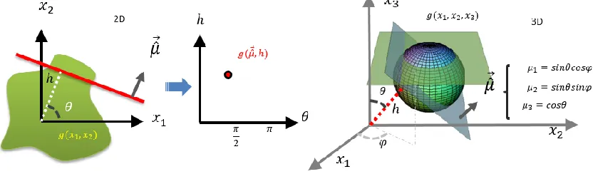
One such method that we propose to use in this thesis work is called Radon’s transform method (Deans 2007). Radon’s transform is an elegant technique that helps in transformation of any 3D images into 2D planes and any 2D image into 1D line. Hence, this technique is heavily applied in the field of computed tomography (CT) and 3D image reconstruction from a cluster of 2D projection images taken on different planes. The transformation of 3D function into multiple functions projected on 2D planes is made possible by Radon transform by the parameterization of the orientation of the planes. Contrary to that, the transformation of images on the 2D planes to a 3D image is made possible by inverse Radon transform. Hence in our case, a forward radon transform is utilized in transferring a 3D function to a 2D function, parameterized by the definition of the 2D planes.

(44)

transform (Banerjee and Kundu 2007) of any function 𝑔(𝐱), which is defined and absolutely integrable over all space, can be written as

𝑔̃(𝛍⃗⃗ , ℎ) = 𝑅{𝑔(𝐱⃗ )} = ∫ 𝑔(𝐱)𝛿(ℎ − 𝛍̂⃗⃗ . 𝐱⃗ )𝑑Ω̂ (15)

Where 𝑑Ω is the volume element and equation (15) is a surface integral over the plane ℎ = 𝜇_𝑘𝑥_𝑘. The physical meaning of the integral could be briefly described in 2D and 3D using the Fig. 4.8. In case of 2D, the infinite numbers of lines can be defined as the function of distance ℎ from the origin with their local orientation of the lines designated by their unit normal 𝛍̂⃗⃗ such that each line can be represented by a point in the Radon space. Similarly, in case of 3D, the infinite numbers of planes can be defined as the function of distance ℎ from the origin with their local orientation of the planes designated by their unit normal 𝛍̂⃗⃗ such that 3D image can be represented by a 2D plane in the Radon space. The Dirac 𝛿 function in eq. 15 signifies that the values exist only on the plane 𝛍⃗⃗ , ℎ̂ and everywhere else the integral ceases to exist, i.e., it is zero.

(45)

Radon transform has many elegant features. However, here we mention few of them that was adopted in the process of transforming the partial differential equation (Eq. 14) into the coupled ordinary differential equations. Those features are as follows.

Radon transform of derivatives of a function (Wang 1994) can be written as

𝑅 {( 𝜕2𝑔

𝜕𝑥𝑖𝜕𝑥𝑗)} = 𝜇𝑖𝜇𝑗

𝜕𝑔̃(ℎ,𝛍)

𝜕ℎ2 (16)

Moreover, the inverse Radon transform of the above equation (Wang 1994) can be written as

𝑔(𝐱, ω) = − 1

8𝜋2∭

𝜕2𝑔̃(ℎ,𝛍) 𝜕ℎ2 |

ℎ=𝛍.𝐱 𝑠𝑝ℎ𝑒𝑟𝑒

|𝛍|=1 𝑑Ω(𝛍) (17)

We use these identities in our forthcoming calculations. After applying the Radon transform on the eq. 14 we get coupled ordinary differential equations.

Γ_𝑖𝑚𝑑2𝑔̃𝑚𝑝

𝑑ℎ2 + 𝜔2𝛿𝑖𝑚𝑔̃𝑚𝑝 = −𝛿𝑖𝑝

𝑓𝑝(𝜔)

𝜌 𝛿(ℎ) (18)

Γ_𝑖𝑚 =𝐶𝑖𝑗𝑚𝑙𝜇𝑗𝜇𝑙

𝜌 ; 𝐵𝑚𝑗𝐵𝑗𝑝 = 𝜔

2_Γ

𝑖𝑚−1 (19)

(46)

𝑔̃_𝑚𝑝 = 𝑖

𝜔2_𝜌𝑓𝑝𝐵𝑗𝑝𝑒

𝑖ℎ𝐵𝑚𝑗_{; ℎ > 0} ₍₂₀₎

Further applying the spectral theorem, we can write an analytic function L which is a function of the Γ𝑖𝑚 matrix in the following form

𝐋(Γ𝑖𝑚) = ∑𝑛𝑧=1𝐋(𝛾𝑧)(𝑃𝑖𝑚)(𝑧) (21)

Where z is the index is eigenvalues for the summation and n is the total number of eigenvalues in the system. Since in our case we have three eigenvalues, hence 𝑛 = 3. 𝛾𝑧 is

the z-th eigen value and (𝑃_𝑖𝑚)(𝑧) is the projection matrix of the z-th eigen mode. The correspondence between the eigen modes with the wave velocities 𝐶_𝑞𝐿, 𝐶_𝑞𝐹𝑆, 𝐶_𝑞𝑆𝑆, their eigen vectors 𝛗_𝐋, 𝛗_𝐅𝐒, 𝛗_𝐒𝐒, respectively and the new parameter defined as 𝛾_𝑧 and (𝑃_𝑖𝑚)(𝑧) can be explicitly written as follows

𝛾₁ = (𝐶_𝑞𝐿)2 ; 𝛾₂ = (𝐶_𝑞𝐹𝑆)2 ; 𝛾₃ = (𝐶_𝑞𝑆𝑆)2 (21)

(𝑃_𝑖𝑚)(1)_{= 𝜑}

𝐿𝑖𝜑𝐿𝑚 ; (𝑃𝑖𝑚)(2)= 𝜑𝐹𝑆𝑖𝜑𝐹𝑆𝑚 ; (𝑃𝑖𝑚)(3) = 𝜑𝑆𝑆𝑖𝜑𝑆𝑆𝑚 (22)

Based on these understanding, by the application of spectral resolution theorem, we can further write the analytic transformed displacement function as

𝑔̃_𝑚𝑝 = 𝑖

𝜔2_𝜌𝑓𝑝∑

𝜔 √𝛾𝑧𝑒

𝑖ℎ(𝜔

√𝛾𝑧)

3

𝑧=1 (𝑃𝑚𝑝)

(𝑧)

(23)

Now applying the inverse Radon transform, we get the displacement Green’s function (Yeatts 1984) in the frequency domain

𝑔𝑚𝑝(𝑥𝑛, 𝜔) = 𝑖𝜔

8𝜋2_𝜌𝑓𝑝∑ ∭ 𝐻𝑧(𝜇𝑖𝑥𝑖)

(47)

Where, 𝐻_𝑧(𝜇_𝑖𝑥_𝑖) is the Heaviside step function which implies that the integral only exists for 𝜇_𝑖𝑥_𝑖 ≥ 0 and it vanishes for 𝜇_𝑖𝑥_𝑖 < 0. Hence the integral in eq. 24 is valid only when the angle between the direction of wave propagation and the Radon’s plane is less than or equal to 900_{. To add to that, we can say that the intended direction between a source}

and a target and the reduced 2D Radon planes will make a hemisphere, inside which the integral (eq. 24) is valid. This equation ep. 24 is the expression for the displacement Green’s function in frequency domain.

However, we want an even more simplified expression for the Green’s function. To achieve that, we shall revisit the eq. 12. By substituting the corresponding relation discussed in eq. 21 and applying the spectral theorem, following the simplification, we can express the inverse of the Christoffel’s operator 𝐋𝑚𝑝(𝑘𝑛, 𝜔) as follows

𝐋_𝑚𝑝(𝑘_𝑛, 𝜔)−1 _{= ∑} 𝜑𝑚𝑖(𝑧)𝜑𝑖𝑝(𝑧)

𝜌𝛾𝑧|𝑘|2−𝜌𝜔2

3

𝑧=1 = ∑

𝛾𝑧−1(𝑃𝑚𝑝) (𝑧)

𝜌(|𝑘|2_−𝜔2_/𝛾 𝑧)

3

𝑧=1 (25)

By substituting Eq. 25 into the Eq. 12, we get an alternative expression for the displacement Green’s function which we can write as follows.

𝑔_𝑚𝑝(𝑥𝑛, 𝜔) =

𝑓_𝑝

(2𝜋)3∑ ∭ [(𝑠𝑧)2(𝑃𝑚𝑝) (𝑧) 𝑠𝑖𝑛𝜃𝑑𝜃𝑑𝜙] 𝑠𝑝ℎ𝑒𝑟𝑒 |𝐫|=1 3 𝑧=1 ×

∫ [exp (−𝑖|k| 𝑥1𝑠𝑖𝑛𝜃𝑐𝑜𝑠𝜙+𝑥2𝑠𝑖𝑛𝜃𝑠𝑖𝑛𝜙+𝑥2𝑐𝑜𝑠𝜃)

(|𝑘|2_−𝜔2_(𝑠

𝑧)2) ]

∞

−∞ 𝑘

2_𝑑𝑘 ₍₂₆₎

(48)

However, in eq. 26, the latter part of the integral has a pole at |𝑘|2 = 𝑎2 , where

𝑎 = 𝜔𝑠𝑧 which can be simplified by the application of the following identity known as

Cauchy’s integral formula (Every, Pluta et al. 2004).

∫ exp (𝑖𝑘𝑢)_(𝑘2_−𝑎2₎

∞

−∞ 𝑘

2_{𝑑𝑘 = 𝜋𝑖𝑎𝑒}𝑖𝑎|𝑢|_{+ 2𝜋𝛿(𝑢)} ₍₂₇₎

Substituting the Cauchy’s integral identity (Eq. 27) into Eq. 26 and performing mathematical simplifications, we get the final expression for the displacement Green’s functions in the frequency domain.

𝑔_𝑚𝑝(𝑥_𝑛, 𝜔) = 𝑖𝜔𝑓𝑝

2(2𝜋)2_𝜌∑ ∭ [(𝑠𝑧) 3_(𝑃

𝑚𝑝) (𝑧)

exp(𝑖(𝑘_𝑖𝑥_𝑖)(𝑧)_{) 𝑠𝑖𝑛𝜃𝑑𝜃𝑑𝜙]} 𝑟=1 𝜃=𝜋; 𝜙=2𝜋

𝑟=0 ; 𝜃=0; 𝜙=0 3

𝑧=1

+ 1

2(2𝜋)2_𝜌|𝐱|∫ (𝑠𝑧)

2_(𝑃 𝑚𝑝)

(𝑧)

𝑑𝜙

2𝜋

0 (28)

(49)

Fig 4.9. A schematic diagram to visualize the integral in Eq. 28.

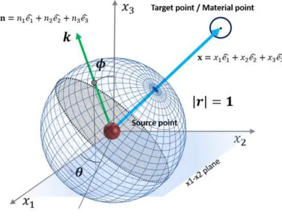
It is required to calculate the wave field in the intended direction of wave propagation (blue arrow) at any target point (black dot with blue ring) due to any source point (red sphere). For that purpose, the influence of the wave field at the target due to all three wave modes in all possible wave direction (green arrow) is considered. Also, only the forward propagating waves, i.e., the grid points on the sphere above the midplane (gray plane) are considered which is similar to the existence of Heaviside step function in Eq. 24. Furthermore, the normal to the gray plane can be visualized as a radon plane ℎ = 𝜇_𝑘𝑥_𝑘

in Fig. 4.9 where 𝜇_𝑘is identical to 𝑛_𝑘. The second part of the integral in Eq. 28 pertains to the perimeter of the circle on the midplane (gray plane) perpendicular to the blue arrow.

(50)

of understanding of the equation; we write 𝑔_𝑚𝑝 = 𝑢_𝑚𝑝 . Before we can calculate the stress Green’s Function, we need to calculate the strain.

The strains at the target point can be calculated with the help of strain-displacement relation which requires taking the spatial derivative of the displacement Green’s functions obtained from the eq. 28. The expression is as follows.

𝜀𝑝_𝑚𝑗 = 1

2(𝑢𝑚,𝑗 𝑝

+ 𝑢_𝑗.𝑚𝑝 ) (29)

Finally, to calculate the stress Green’s Function tensor for a specific direction of point force along p, we will use the constitutive equation for the anisotropic medium given by,

𝜎𝑝

𝑖𝑘(𝐱) = 𝐶𝑖𝑘𝑚𝑗𝜀𝑝𝑚𝑗(𝐱) (30)

Where,



p_ik is the stress tensor at the target point (x) due to the source point with force along the p-th direction.

(51)

CHAPTER 5 NUMERICAL COMPUTATION OF GREEN’S FUNCTION

Now that we have the mathematical derivation required for the calculation of the displacement and stress Green’s Functions, we can proceed with the modeling of the wave field in anisotropic media. However, before that, we want to make sure that the implementation of Green’s function into MATLAB code is verified. Also, we also want to understand the physical meaning of the Green’s function as well as visualize the behavior of materials with different types of anisotropy. Therefore, we first calculate the Green’s function for materials that we already considered in chapter 3, a) Transversely isotropic, b) Fully orthotropic, c) Monoclinic material and compare it to the isotropic material, aluminum to see the difference between the isotropic and anisotropic material. For that purpose, we consider two geometric configurations as shown in Fig. 5.1.

(52)

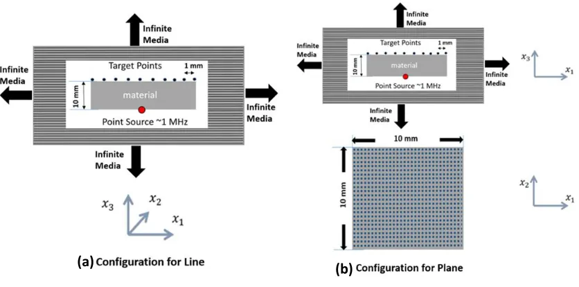
Fig. 5.1. Schematics of configurations to calculate the Green’s function a) for a line b) for a plane

Fig. 5.2. Numerical computation of displacement Green’s function (unit mm) due to forces acting along 1, 2 & 3directions in Fig 5.1a when the inside material is Isotropic. a) displacements along 𝑥₁direction, b) displacements along 𝑥₂direction c) displacements along 𝑥₃direction

(a) (b) (c)

(53)

Fig. 5.3. Numerical computation of displacement Green’s function (unit mm) due to forces acting along 1, 2 & 3directions in Fig 5.1a when the inside material is Transversely Isotropic. a) displacements along 𝑥₁direction, b) displacements along 𝑥₂direction c) displacements along 𝑥₃direction

Fig. 5.4. Numerical computation of displacement Green’s function (unit mm) due to forces acting along 1, 2 & 3directions in Fig 5.1a when the inside material is Fully Orthotropic. a) displacements along 𝑥₁direction, b) displacements along 𝑥₂direction c) displacements along 𝑥₃direction

(a) (b) (c)

(54)

Fig. 5.5. Numerical computation of displacement Green’s function (unit mm) due to forces acting along 1, 2 & 3directions in Fig 5.1a when the inside material is Monoclinic. a) displacements along 𝑥₁direction, b) displacements along 𝑥₂direction c) displacements along 𝑥₃direction

If we look at the displacement Green’s function plot for line configuration (fig 5.2 – 4.5), we see that for the isotropic material, the displacements are maximum at the center, i.e., at the closest proximity to the point source actuation and decays along either side. Similarly, for the transversely isotropic material assuming a composite, the displacements are not maximum at the center. Instead, it bifurcates along the fiber direction. Also, we can see the various behavior depicted by the orthotropic and monoclinic material. Since the behavior illustrated agree to our theoretical understanding of the material, the implementation of Green’s function is verified.

Now to further enhance our numerical computation and understanding of the Green’s function, we calculate the Green’s function for a plane or rectangular domain. In the Fig. 5.1 b, we have a configuration for calculation of the displacement and stress Green’s function in an arbitrary plane inside the Transversely Isotropic material. The configuration is composed of 51 X 51 target points with a spacing of 1mm in a square plane of 10 mm X 10 mm and point source with an excitation frequency of 1MHz. The plane of target points and point source is separated by a distance of 2 mm. The stress and

(55)

displacement Green’s function is numerical computed and plotted as a contour plot along the plane of target points.

Based on the displacement and stress Green’s functions (Fig. 5.6 – 5.8), we were able to understand that the Green’s function represents the influence of the source with unit load at any arbitrary target point in the space as well as its dependency on the material property. Also, we also enriched our numerical computation and can finally progress with the calculation of ultrasonic wave field in an anisotropic solid, when the bounded ultrasonic beam is generated from 1 MHz ultrasonic transducer.

Fig.5.6. Numerical computation of displacement Green’s function (unit mm) in Transversely Isotropic material a) 𝑔11 b) 𝑔22 c) 𝑔33 d) 𝑔31 𝑜𝑟 𝑔13 e) 𝑔32 𝑜𝑟 𝑔23 f)

𝑔₂₁ 𝑜𝑟 𝑔₁₂

(a) (b) (c)

(56)

Fig. 5.7. Numerical computation of Stress Green’s function (unit GPa) in the Transversely Isotropic material due to source actuating along 1-direction. a) 𝜎₁₁ b) 𝜎₂₂ c) 𝜎₃₃ d)

𝜎₃₂ 𝑜𝑟 𝜎₂₃ e) 𝜎₃₁ 𝑜𝑟 𝜎₁₃ f) 𝜎₂₁ 𝑜𝑟 𝜎₁₂

Fig. 5.8. Numerical computation of Stress Green’s function (unit GPa) in the Transversely Isotropic material due to source actuating along 3-direction. a) 𝜎₁₁ b) 𝜎₂₂ c) 𝜎₃₃ d)

𝜎 𝑜𝑟 𝜎 e) 𝜎 𝑜𝑟 𝜎 f) 𝜎 𝑜𝑟 𝜎

(a) (b) (c)

(d) (e) (f)

(a) (b) (c)

(57)

CHAPTER 6 NUMERICAL COMPUTATION OF WAVE FIELD WITH THE

IMPLEMENTATION OF DPSM

For numerically computing the wave field in anisotropic media, we institute the analytical model developed for the Green’s function into a numerical technique called Distributed point source method (DPSM). Therefore, we first provide a brief introduction to DPSM. DPSM is a recently developed mesh-free semi-analytical technique developed by Placko and Kundu (Placko and Kundu 2001, Placko, Kundu et al. 2002). They used the technique to model the wave propagation in fluid media, and the technique was further developed by Banerjee (Banerjee and Kundu 2007) to model the isotropic solids. DPSM is used because it helps to overcome the limitations such as the inability to correctly model critical reflection phenomena, failure to adapt to the change in the interface curvature and necessity of far-field approximation. In DPSM, the Green’s function is essential to calculate the displacement and stress profile and simulate the wave propagation behavior.

(58)

is calculated by satisfying the boundary and the interface continuity conditions as required. Finally, displacement and stress profile in the anisotropic medium and the pressure profile in the fluid medium can be calculated with the help of the source strengths.

Fig. 6.1. a) the total field at A is calculated by superposing the contribution of all point sources distributed along the boundary of the anisotropic medium. b) the three mutually perpendicular forces that are contained in the point source.

6.1 Numerical Computation of Wavefield in Anisotropic Half-space

(59)

point sources to the points of interest (C, D). The total ultrasonic field at any arbitrary point C in the anisotropic solid is produced by the superposition of the strength of all the point sources denoted by 𝐀_𝐼∗ whereas the total ultrasonic field at any arbitrary point D in the fluid is produced by the superposition of the strength of all the point sources denoted by

𝐀_𝑠 and 𝐀_𝐼. However, at the moment those source strengths required are unknown. Pertaining to the modeling of the current problem, the length of the interface is taken to be 10mm and 115 point sources were distributed on either side of the interface following the wave length - source diameter rule explicitly described in the previous articles (Banerjee 2007, Banerjee and Kundu 2007). A 1 MHz transducer with the diameter of 2 mm is submerged in to the water and 100 point sources were distributed concentrically just below its transmitting face. The distance between the transducer and interface is taken as 5 mm. For the actuation of transducer, unit velocity is prescribed on the transducer face.

(60)

First, to calculate the unknown source strengths, we need to solve the satisfied boundary conditions (Banerjee 2007, Banerjee and Kundu 2007). If we assume the normal velocity at the transducer face to be V_S₀, the boundary condition on the transducer surface can be written as

0

SS S SI I S

M A M A V (31)

The displacement normal at the fluid-anisotropic interface should be continuous.

*

3_IS _S 3_II _I 3_II _I*

DF A DF A DS A (32)

Also, the normal compressive stress in the anisotropic and pressure in the fluid should be continuous at the interface.

Q A_IS _SQ A_II _I  S33_II_*A_I* (33)

The shear stresses in the anisotropic medium should vanish at the interface.

*

31 * 0 32 * 0

II I

S A



 (34)

Where, M represents the velocity Green’s function matrix in the fluid, Q represents the pressure Green’s function matrix in the fluid, S33, S31 and S32 represents the stress Green’s function matrix in the anisotropic material for 𝜎₃₃ , 𝜎₃₁and 𝜎₃₂, respectively. DF3

is the displacement Green’s function matrix in the fluid in the 𝑥₃ direction, u3 is the displacement Green’s function in the solid in the 𝑥3 direction. SS means the wave field on

(61)

interface I due to the source layer I*. By solving the equations (31), (32), (33), (34) as shown in matrix form (Banerjee and Kundu 2007, Banerjee, Kundu et al. 2007) below, we can calculate the source strengths.

0 * 1 * * * 0 33 0

3 3 3

* 0

0 0 31

0 0 32

SS SI

S S

IS II II

I

IS I II

I II

II

M M

A V

Q Q S

A

DF DF DS

A S S    _{    }  _{    }   _ _{ } _  _{ } _{ } _           (35)

From the matrix equation Eq. 35, we can see that to implement the standard procedure of DPSM (Banerjee 2007, Banerjee and Kundu 2007), the Green’s function for both the fluid and the solid media needs to be computed.

Hence, the Green’s function terminologies required needed for the formulation of DPSM is put together for the convenience and computation of wave field in the respective domains.

6.1.1 Expressions for Velocity, Pressure and Displacement Green’s Function

in fluid

(62)

1 1 2 2 1 1

1 1 1 1 1 1 1 1

1 1 2 2 1 1

2 2 2 2 2 2 2 2

1 1 2 2 1 1

3 3 3 3 3 3 3 3

1 1 2 2

( , ) ( , ) ... ( , ) ( , ) ( , ) ( , ) ... ( , ) ( , ) ( , ) ( , ) ... ( , ) ( , )

... ... ... ... ... ( , ) ( , ) ... (

N N N N

t t t t

N N N N

t t t t

N N N N

t t t t

tM M tM M tM

f x r f x r f x r f x r

M f x r f x r f x r f x r

f x r f x r f x

       1 1 , ) ( , )

N N N N

M tM M MXN

r f x r

                 

Where, ( , ) exp( ₂ )( 1 )

( )

m m

tn f n

m m

tn n m f m

n n

x ik r

f x r ik

i r r

 

1 2

1 1 1

1 2

2 2 2

1 1 1

2 2 2

1 2

1 1 1

exp( ) exp( ) exp( )

... ...

... ... ... ... ... ... ... ... ... ...

... ...

M

f f f

M

f f f

M

f N f N f N

N N N

ik r ik r ik r

r r r

Q

r r r

                      

 NXM

 

1 1 2 2 1 1

1 1 1 1 1 1 1 1

1 1 2 2 1 1

2 2 2 2 2 2 2 2

1 1 2 2 1 1

3 3 3 3 3 3 3 3

1 1 2 2

( , ) ( , ) ... ( , ) ( , ) ( , ) ( , ) ... ( , ) ( , ) ( , ) ( , ) ... ( , ) ( , )

... ... ... ... ... ( , ) ( , ) ... (

N N N N

t t t t

N N N N

t t t t

N N N N

t t t t

tN N tN N

g R r g R r g R r g R r

DFt g R r g R r g R r g R r

g R r g R r g R

       1 1 , ) ( , )

N N N N

tN rN g RtN rN _NXM

                 

Where ( ) 1₂ 1 ₂ ( ) m f n m f n ik r ik r

m m m m

in n f in m in

n

e

g R r ik R e R

r r            ; m m

m in in

in m in x y R r 

 ; t i, 1, 2,3

6.1.2 Expressions for Displacement and Stress Green’s Function in

Anisotropic Solid

(63)

displacement Green’s Function eq. 28 and stress Green’s Function eq. 30 which are written below.

𝑔_𝑚𝑝(𝑥_𝑛, 𝜔) = 𝑖𝜔𝑓𝑝

2(2𝜋)2_𝜌∑ ∭ [(𝑠𝑧)3(𝑃𝑚𝑝) (𝑧)

exp(𝑖(𝑘_𝑖𝑥_𝑖)(𝑧)_{) 𝑠𝑖𝑛𝜃𝑑𝜃𝑑𝜙]} 𝑟=1 𝜃=𝜋; 𝜙=2𝜋

𝑟=0 ; 𝜃=0; 𝜙=0 3

𝑧=1

+ 1

2(2𝜋)2_𝜌|𝐱|∫ (𝑠𝑧)

2_(𝑃 𝑚𝑝)

(𝑧)

𝑑𝜙

2𝜋

0 (28)

𝜀𝑝

𝑚𝑗 =

1 2(𝑢𝑚,𝑗

𝑝

+ 𝑢_𝑗.𝑚𝑝 ) (29)

𝜎𝑝_𝑖𝑘(𝐱) = 𝐶_{𝑖𝑘𝑚𝑗}𝜀𝑝_𝑚𝑗(𝐱) (30)

1 1 1

2 2 2

1 2

3 3 3

1 2

3 3 3

1 2

3 3 3 3

... ... ... ... 3 ... ... ... ... ...

... ... ... ... ... ... ...

N N N

M

M NX M

g g g

DS

g g g

                

where, ₃mn [ ₃₁m ₃₂m ₃₃m]

n

g  g g g

1 1 1

2 2 2

1 2

3 3 3

1 2

3 3 3

1 2

3 3 3 3

... ... ... ... 3 ... ... ... ... ...

... ... ... ... ... ... ...

N N N

M

i i i

M

i i i

M

i i i NX M

s s s

S i

s s s

                

where, ₃mn [ ₃m ₃m ₃m]

i i i i n

s     and i1, 2,3

(64)

After obtaining the source strengths, we can now compute the wave field for the anisotropic half space media. As we have mentioned before, we compute the wave field for three different types of anisotropic material: a) Transversely isotropic, b) Fully orthotropic, c) Monoclinic material.

6.2 Processes to Speed up the Computation

6.2.1 Sequential Mapping of Poly-Crepitus Green’s Function

(65)

(66)

Please visit the code named Aniso_green.m in the appendix for the detailed implementation and understanding of the technique.

Fig. 6.3: A schematics showing the sequential mapping of Green’s function, a) source and target point combinations b) extended target points in 2D c) Calculated Green’s function on extended point sources d) Assignment of Green’s function for an edge source e) source-target combinations in 3D, f) sequential mapping of 3D Green’s function.

6.2.2 Maximizing the Discretization Angle for Anisotropic Green’s function