An Innovative MATLAB Based Approach to Analyse the Performance of Solar PV Module

An Innovative MATLAB Based Approach to

Analyse the Performance of Solar PV Module

P. Narayan Sinha1, S. Choudhury2

Assistant Professor, Dept. of EE, GIMT, Guwahati, Assam, India1 Assistant Professor, Dept. of EE, GIMT, Guwahati, Assam, India1

ABSTRACT: The solar energy seems to be one of the most readily available, non polluting renewable source of energy which can be directly converted into electricity using the photovoltaic (PV) module. The overall performance of the solar cell changes with varying weather conditions like irradiance, temperature, shading conditions etc. So any changes in the input parameters (irradiance, temperature etc.) to this module immediately imply the changes in the output parameters (current, voltage, power or other) and does affecting the efficiency and corresponding fill factor of the module. In order to analyse the random changes in the output characteristics of the PV cell with varying weather conditions, we have chosen a single diode model. The model is implemented using MATLAB software and the simulated results have been validated using BP SX 150S PV module in standard test conditions (STC). In this paper the MPPT (maximum power point tracking) algorithm simulation results are also presented. It is envisaged that this approach can be very useful for researchers to quickly and easily determine the performance of any PV module, the delivery of to track the maximum power point and to design their systems.

KEYWORDS: Solar energy, PV module, irradiance, I-V characteristic, P-V characteristic, short circuit current, open circuit voltage, standard test conditions, ideality factor, fill factor.

I.INTRODUCTION

Energy resource is one of the most important factor in today’s modern world to keep working smoothly. As energy crisis is one of the major problem presently that the world is facing, so it is time to shift focus towards renewable energy sources. Among the renewable energy resources, the energy through the photovoltaic (PV) effect can be considered the most essential and prerequisite sustainable resource because of the ubiquity, abundance, and sustainability of solar radiant energy [1]. Photovoltaic system emerged as a main alternative for the decentralized power generation in the world [2]. Due to high cost of the PV module, it is of need to implement an accurate and reliable simulation model to thoroughly investigate the non-linear I-V, P-V curves of the designed model under varying surrounding conditions prior to installation.

II.MODELING A PV CELL

Single diode model is the simplest way to represent the solar cell. Fig 1 (a) shows the single diode model with Rs and Fig 1 (b) shows the single diode model with Rs and Rp.

Fig. 1(a) Single diode model with series resistance (Rs) Fig. 1(b) Single diode model with series resistance

This model consists of a photo current source, one diode parallel to source, series resistance (Rs) and parallel resistance (Rp). The current generated by the photon is represented by the current source (often denoted as Iph , Ipv or IL ).

Three important operating points of single diode solar cell are short circuit current (Ish), open circuit voltage (Voc) and the maximum power point (MPP). Fig-2 shows all these three points.

Fig. 2 I-V characteristic showing Isc, Voc & MPP

As shown in fig-3(a), shorting together the terminals gives short circuit current (Ish) and in this case,

Iph= Ish (i.e. short circuit current is equal to photon generated current).

When there is no connection to the PV cell (open circuit) as shown in fig-3(b) gives open circuit voltage (Voc). The values of these parameters are generally provided by the PV cell/module manufacturers in their datasheets.

Fig. 3(a) Short circuit current Fig. 3(b) Open circuit voltage

Fig. 4 PV cell with a load and its simple equivalent circuit [3]

Using KCL in the equivalent circuit of fig-4, the output current (I) in the PV cell is found as

I = I exp −1 --- (2)

where Isc is the short circuit current (= Iph) Id is the diode equation,

Io is the reverse saturation current of diode (A), Vd is the voltage across the diode (V),

K is the Boltzmann’s constant (1.381x 10 -23 J/K), q is the electron charge (1.602 x 10 -23 C), T is the junction temperature in Kelvin (K)

Using equation (2) in equation (1) gives-

I = Isc – I exp −1 --- (3) where V is the voltage across the PV cell and I is the output current of the PV cell.

In open circuit condition, I = 0, equation (3) becomes ,

0 = Isc – I exp −1 --- (4)

I0 = --- --- (5)

The reverse saturation current of diode (I0) is constant under constant temperature and keep on changing with the

change in temperature. To a very good approximation, the photon generated current, which is equal to Isc, is directly proportional to the irradiance, the intensity of illumination, to PV cell [4].

The value of Isc (obtained from the manufacturer datasheet) under standard test conditions, G0 = 1000 W/m^2 at the air

mass (AM) = 1.5 helps in finding the Isc value at any other irradiance value (G in W/m^2) as given below:

Isc| = . Isc| --- (6)

The voltage-current relationship of a PV cell is given by

I = I −I exp ( . ) −1 − . -- --- (7)

where n is the ‘ideality factor’

III.MODELING OF PV MODULE

Fig. 5 PV cells are connected in series forming a PV module

Here the BP SX 150S PV module has been chosen for MATLAB simulation model to ratify the system under irradiation and temperature variation. The module consists of 72 multi-crystalline silicon solar cells in series and provides 150W of maximum nominal power [5]. Table-1 below shows the electrical specification of the test module.

Table 1: Electrical characteristics data of PV module taken from the datasheet [5]

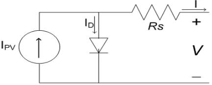
Fig. 6 The equivalent circuit used in the MATLAB simulation

Fig-6 shows the equivalent circuit used in this simulation. The PV efficiency is sensitive to small change in Rs but insensitive to variation in Rp. For a PV module or array, the series resistance becomes apparently important and the shunt down resistance approaches infinity which is assumed to be open [1]. So in this model considering the effect of parallel resistance (Rp) is not included and thus letting Rp= ∞ and using this value in equation (7), gives the current-voltage relationship of the PV cell as

I = I −I exp ( . ) −1 --- (8)

Electrical Characteristics BP SX 150S PV

Maximum Power (Pmax) 150 W

Voltage at Pmax (Vmp) 34.5 V

Current at Pmax (Imp) 4.35 A

Open circuit voltage (Voc) 43.5 V

Short circuit current (Isc) 4.75 A

Temperature coefficient of Isc 0.065 ± 0.015 %/ 0C Temperature coefficient of Voc -160 ± 20 mV/ 0C Temperature coefficient of

power

-0.5 ± 0.05 %/ 0C

where I is the PV cell current which is same as the PV module current, V is the PV cell voltage (= PV module voltage / no of cells in series), T is the PV cell temperature in Kelvin

The short circuit current at any given cell temperature is given by

Isc| = [1 +α(T−T )]. Isc| - --- (9)

where Isc at Tref is 4.75A as per the datasheet,

Tref is the reference temperature in Kelvin i.e. 298K as per datasheet,

α is the temperature coefficient of Isc as per datasheet

The short circuit current at any given irradiance is given by equation no (6)

Isc| = . Isc| --- (10)

The reverse saturation current of diode including the ideality factor at Tref is obtained from equation no (5) as

I0 =

--- (11)

The reverse saturation current of diode at a given temperature T is given as [6]

I | = I | . exp ( − ) --- (12)

where Eg is the band gap energy of the semiconductor (for Si, 1.12eV)

The value of the series resistance (Rs) is calculated by evaluating the slope dI/dV of the I-V curve at the Voc [6]. Differentiating equation no (8) and then rearranging the value of Rs can be found as in equation no (13).

dI = 0−I .q .

e . --- (13)

R =− − ---(14)

Finally, the equation of the I-V characteristics is solved from equation no (8) using Newton Raphson’s (N-R)method which is widely used for obtaining roots of implicit transcendental equations, is popular in iterative computational applications because of its simplicity and fast convergence [7, 8].

The N-R method is described as

x = x − ( )

′( ) --- (15)

where f ' (xn) is the derivative of the function f(x) = 0,

xn is the present value and x n+1 is the next value

The following function is obtained using equation no (8)

( ) = − − . −1 = 0 --- (16)

I = I −

.

.

. --- (17)

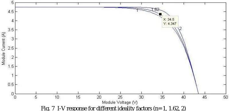
The PV module is implemented in MATLAB environment using all the equations (8-17). Another important factor in modelling the PV module is the diode ideality factor (n) and after several trials in MATLAB model (fig-7) its value is chosen to be 1.62.

IV.SIMULATION RESULT AND DISCUSSION

The test model of PV module is implemented in MATLAB environment whose input parameters are ambient parameters like irradiance and temperature and output are panel current, voltage, power etc. The simulated responses are used to validate the functionality of the module implemented comparing with the test module specifications.

The simulated response as shown in fig-7, shows the variation of the I-V curve considering different ideality factors (1, 1.62 and2) and its value for modelling is chosen to be 1.62 as the response at this value provides close agreement with the response provided in the datasheet.

Fig. 7 I-V response for different ideality factors (n= 1, 1.62, 2)

Fig. 8 I-V response in standard test condition (T=250C, G=1000W/m^2)

Fig. 9 P-V response in standard test condition (T=250C, G=1000W/m^2)

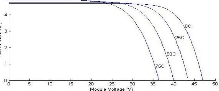
In this work, two types of simulations are carried out- one is under constant irradiance (1000W/m^2) and varying temperature (00C, 250C, 500C and750C) and the other is at constant temperature (250C) and varying irradiance (200W/m^2, 400W/m^2, 600W/m^2, 800W/m^2 and 1000W/m^2). Figure (10-14) shows the simulation results under these two conditions.

Fig-10, 11 illustrates the dependence of I-V characteristics on temperature and irradiance.

Fig-10 reveals that with the increase in temperature the rate of photon generation increases thus reverse saturation current increases rapidly and this results on reduction in band gap. Hence this leads to marginal changes in current but major changes in voltage [9].

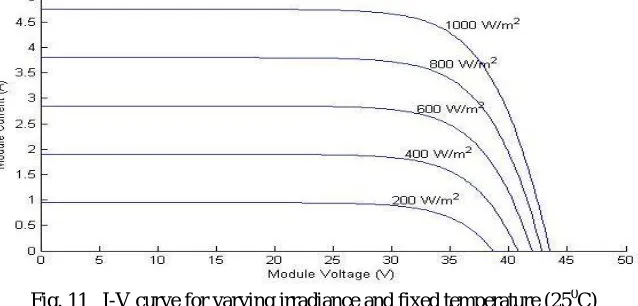
Fig. 11 I-V curve for varying irradiance and fixed temperature (250C)

From Fig-11, it is clear that photon generated current depends on the irradiance. Higher the irradiance, greater is the current generation and while voltage is not varying much.

Fig-12 presents the PV curve under different temperatures and fixed irradiance while Fig-13 presents the PV curve under different irradiance and fixed temperature.

Fig. 12 P-V curve for varying temperature and fixed irradiance (1000W/m^2)

From figures (10&12), it is clear that, when the operating temperature increases, the current output increases marginally but the voltage output decreases drastically, which result in net reduction in power output with a rise in temperature [10].

It is also observe that, the short-circuit current and the maximum power output of the PV module increase with the increase of irradiance as shown in Figure (11&13). The reason is the open-circuit voltage is logarithmically dependent on the solar irradiance, yet the short-circuit current is directly proportional to the radiant intensity [1].

Fig. 14 P-V curve showing Maximum power point tracking in varying irradiance and fixed temperature (250C) With the help of MPPT algorithms, the simulated response for automatically tracking the maximum power point in P-V curves for different irradiance and constant temperature (t=250C) is shown in fig-14.

FF indicates the performance of a solar cell which is expressed as- FF = .

Higher the FF (approaching towards unity), better is the performance quality of the solar cell which is represented with the help of fig-15. As shown in fig-15, fill factor 0.7275 gives the best performance of this module which is practically achievable.

Fig. 15 Fill factor (FF) Vs. Temperature characteristic (G=1000W/m^2)

V. CONCLUSION

based implementation makes this PV model easily designed and scrutinised with the experimental data provided by manufacturer in conjunction with the maximum power point tracking. Simulated results were verified by comparing with the data provided in the datasheet which shows excellent consistency between the simulated data and the manufacturer’s data and thus it proves the effectiveness of the proposed modelling method. Finally, it can be concluded that this model can be used as a tool to test and analyse the behaviour of different PV modules under any irradiation and temperature conditions using standard test conditions.

REFERENCES

[1] Huan-Liang Tsai, Ci-Siang Tu, and Yi-Jie Su, “Development of Generalized Photovoltaic Model Using MATLAB/SIMULINK”, Proceedings of the World Congress on Engineering and Computer Science 2008 WCECS 2008, October 22 - 24, 2008, San Francisco, USA.

[2] K.Jayachandran, A.K.Tiwari, N.R.Raje, O.S.Sastry, “Modeling of Operation of Solar PV Module under Practical Conditions in MATLAB”, International Conference on Signal, Image Processing and Applications With workshop of ICEEA 2011 IPCSIT, vol.21 (2011) © (2011) IACSIT Press, Singapore.

[3] Masters, Gilbert M. Renewable and Efficient Electric Power Systems John Wiley & Sons Ltd, 2004. [4] Messenger, Roger & Jerry Ventre Photovoltaic Systems Engineering 2nd Edition CRC Press, 2003. [5] BP Solar BP SX150 - 150W Multi-crystalline Photovoltaic Module Datasheet, 2001.

[6] Walker, Geoff R, “Evaluating MPPT converter topologies using a MATLAB PV model”, Australasian Universities Power Engineering Conference, AUPEC ‘00, Brisbane, 2000.

[7] F.Cajori,Historical note on the Newton-Raphson method of approximation‖ American Mathematical monthly (1911),18,29-32,on 30. [8] D. Bonkoungou, Z. Koalaga, D. Njomo, “Modelling and Simulation of photovoltaic module considering single-diode equivalent circuit model

in MATLAB”, International Journal of Emerging Technology and Advanced Engineering, Volume 3, Issue 3, March 2013.

[9] Arjyadhara Pradhan, S.M. Ali, Chitralekha Jena, “Analysis of Solar PV cell Performance with Changing Irradiance and Temperature”, International Journal Of Engineering And Computer Science , Volume 2, Issue 1 ,Jan 2013, Page No. 214-220.

[10] M. Abdulkadir, A. S. Samosir and A. H. M. Yatim, “Modeling and simulation based approach of Photovoltaic system in Simulink model”, ARPN Journal of Engineering and Applied Sciences, VOL. 7, NO. 5, MAY 2012.