Scholarship@Western
Scholarship@Western
Electronic Thesis and Dissertation Repository
8-9-2018 10:00 AM
Bubble Dynamics and Dense Phase Composition in 2-D Binary
Bubble Dynamics and Dense Phase Composition in 2-D Binary
Gas-Solid Fluidized Bed
Gas-Solid Fluidized Bed
Tianzi Bai
The University of Western Ontario
Supervisor Zhu, Jesse
The University of Western Ontario Co-Supervisor Barghi, Shahzad
The University of Western Ontario
Graduate Program in Chemical and Biochemical Engineering
A thesis submitted in partial fulfillment of the requirements for the degree in Master of Engineering Science
© Tianzi Bai 2018
Follow this and additional works at: https://ir.lib.uwo.ca/etd
Part of the Complex Fluids Commons, and the Other Chemical Engineering Commons
Recommended Citation Recommended Citation
Bai, Tianzi, "Bubble Dynamics and Dense Phase Composition in 2-D Binary Gas-Solid Fluidized Bed" (2018). Electronic Thesis and Dissertation Repository. 5514.
https://ir.lib.uwo.ca/etd/5514
This Dissertation/Thesis is brought to you for free and open access by Scholarship@Western. It has been accepted for inclusion in Electronic Thesis and Dissertation Repository by an authorized administrator of
i
Gas-solid bubbling fluidized bed with binary particles is a potential candidate for performing
the dry coal beneficiation process due to its advantages such as the ability to adjust separation
density and the elimination of process water. A two-dimensional (2D) fluidized bed was used
to study bubble dynamics and dense phase composition distribution in order to gain some
fundamental understanding of this system. Digital image analysis (DIA) was employed to
measure bubble diameter, bubble rise velocity, bed expansion and particle composition
distribution. Magnetite and sand particles as pure and binary mixtures were used in the
fluidized bed. Bubble diameter and bubble rise velocity both increased with the distance
above the gas distributor and excess gas velocity. Bubble diameter of the binary mixtures is
smaller than that of pure particles. Unlike the binary particles of the same size, bubble
diameter was at its smallest when the amounts of sand and magnetite were almost identical in
the system of binary particles having the same aerodynamic diameter, however the effect was
not appreciable at a higher magnetite particles concentration. Bubble rise velocity was found
to be proportional to the bubble diameter and did not change with axial position for the same
bubble size. Bubble rise velocity increased while ascending in the bed due to an increase in
bubble size. In addition, a preliminary experiment of tracing dense phase composition using
DIA was carried out and a correlation for estimating the bed density based on the dense phase
composition and bed expansion was developed.
Keywords
Dry coal beneficiation, two-dimensional fluidized bed, digital image analysis, bubble diameter,
ii
Acknowledgments
First of all, I would like to give my gratification to my supervisor Dr. Jesse Zhu. Thanks for
giving me an opportunity to study at the University of Western Ontario and carry out my master
project so that I can improve my ability. Furthermore, Prof. Zhu’s profound professional knowledge,
rigorous attitude on studies, strive for self-improvement, instructing others indefatigably and
approachability has had a profound influence on me. In a few conversations with my supervisor, his
opinion on scientific research has given myself a better understanding of my own research, and has
helped me determine my future academic goals.
Thanks to my co-supervisor Dr. Shahzad Barghi for his guidance, valuable suggestions
throughout the whole experiment and for writing for this thesis. His professional experience has
helped me solve many problems during my masters study.
I would like to thank Mr. Chenyang Zhou for his valuable suggestions for my research and Mr.
Bowen Han for his help in MATLAB program. Thanks to Mr. Ziang Guo for his help in data analysis.
Finally, thanks to my family and my boyfriend Mr. Jia Meng. When I faced with difficulties and
challenges, become frustrated, they encouraged me and supported me, let me continue on this journey
without fear.
Here, I express my deep gratitude to the professors, colleagues and my family who helped me
iii
Table of Contents
Abstract ... i
Acknowledgments... ii
Table of Contents ... iii
List of Tables ... vi
List of Figures ... vii
List of Appendices ... x
Nomenclature ... xi
1
Introduction ... 1
1.1
Importance of coal beneficiation ... 1
1.2
Bubbling fluidized bed applied in coal beneficiation ... 3
1.3
Objectives ... 6
2
Literature review ... 8
2.1
Gas-solid fluidization technology applied in coal beneficiation... 8
2.2
Two phase theory ... 9
2.3
Particle segregation and minimum fluidization velocity ... 11
2.4
Bubble size ... 12
2.5
Bubble rise velocity ... 15
2.6
Binary fluidized bed ... 15
3
Experimental set-up and methodology ... 17
3.1
Materials and operating conditions ... 17
3.2
Image processing in bubble dynamics ... 17
3.3
Image processing in tracing dense phase compositions ... 19
3.4
Aerodynamic diameter ... 21
iv
3.6
Bubble size ... 22
3.7
Bubble rise velocity ... 23
3.8
Bed expansion ... 24
3.9
Experimental apparatus ... 24
4
Result and discussion ... 26
4.1
Minimum fluidization velocity ... 26
4.2
Bubble size ... 33
4.2.1
Bubble size distribution ... 33
4.2.2
Bubble size under different operating conditions ... 34
4.2.3
Excess gas velocity, sands volume fraction and sand size effects on bubble
size ... 40
4.3
Bubble rise velocity ... 45
4.3.1
Bubble rise velocity under different operating conditions ... 45
4.3.2
Distance above the gas distributor and bubble size effect on bubble rise
velocity ... 49
4.3.3
Bubble volume fraction... 53
4.4
Bubble coalescence and splitting ... 56
4.4.1
Bubble size and bubble total volume changing during bubble coalescence
... 56
4.4.2
Bubble size and bubble total volume changing during bubble splitting ... 58
4.5
Bed expansion ... 60
4.6
Dense phase composition and the estimation of bed density ... 61
5
Conclusion ... 69
6
Recommendation and future work ... 71
6.1
Recommendation ... 71
6.2
Future work ... 72
v
Appendices ... 79
vi
List of Tables
Table 3.1 Experimental Particles Properties ... 17
vii
List of Figures
Figure 1.1 Primary energy regional consumption by fuel 2018 (Billion ton) (BP statistical
review of world energy) ... 1
Figure 1.2 Primary Fuel Demand in 2018 (Billion ton) (BP statistical review of world
energy) ... 2
Figure 1.3 Carbon emissions by source in 2018 (Billion tones CO
2) (BP statistical review of
world energy) ... 3
Figure 1.4 Forces acting on a coal particle ... 5
Figure 2.1 Diagram of two phase theory in fluidized bed [Han, 2017] ... 10
Figure 2.2 Typical mixing/segregation states. (a) Completely mixed, (b) completely
segregated, (c) partial mixing. [Chiba et al. 1979] ... 11
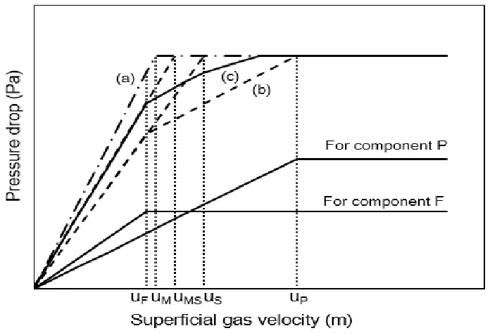
Figure 2.3 Effect of the mixing/segregation state on the relationship between bed pressure
drop and superficial gas velocity (idealized). (a) Completely mixed, (b) Completely
segregated. (c) Partial mixing [Chiba et al. 1979] ... 12
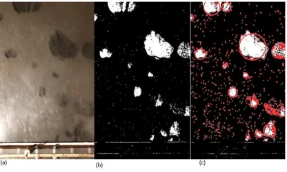
Figure 3.1 Image Processing Procedure (a) Original RGB Image (b) Black and White Binary
Image (c) Image with Circles ... 19
Figure 3.2 Original RGB images in tracing particle composition. (a) Image without obvious
bubbles. (b) Image with obvious bubbles. (c) Image that improve contrast ... 20
Figure 3.3 Histogram of greyscale value distribution ... 21
Figure 3.4 The determination of minimum fluidization velocity using the relationship
between total pressure and superficial gas velocity ... 22
Figure 3.5 Schematic diagram of the bubbling fluidized bed ... 25
viii
Figure 4.1 Determination of minimum fluidization velocities of binary mixtures using
pressure drop versus superficial gas velocity in Magnetite225-Sand225 system ... 26
Figure 4.2 Segregation in the fluidized bed in Magnetite225-Sand225 system ... 27
Figure 4.3 Determination of minimum fluidization velocities of binary mixtures using
pressure drop versus superficial gas velocity in Magnetite225-Sand304 system ... 27
Figure 4.4 Minimum fluidization velocity, complete fluidization velocity and initial
fluidization velocity as a function of sand volume fraction in Magnetite225-Sand225 system
... 29
Figure 4.5 Minimum fluidization velocity as a function of sand volume fraction in
Magnetite225-Sand304 system ... 30
Figure 4.6 Bubble size distribution in axial position ... 34
Figure 4.7 Bubble size distribution in lateral position ... 34
Figure 4.8 Average area equivalent bubble size as a function of distance above the gas
distributor under different excess gas velocity ... 37
Figure 4.9 Average area equivalent bubble size of single-component particles and binary
mixtures... 39
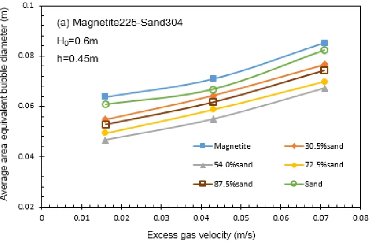
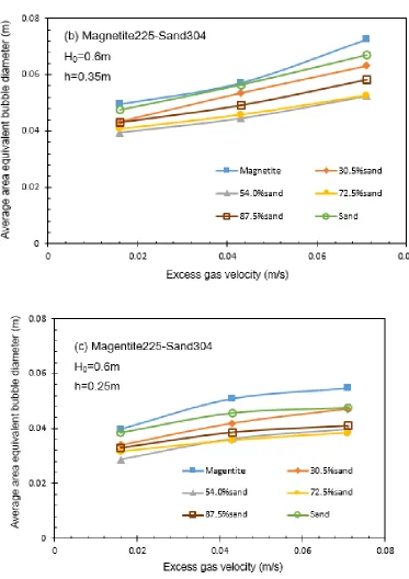
Figure 4.10 Average area equivalent bubble size as a function of excess gas velocity at
different distance above the gas distributor ... 41
Figure 4.11 Average area equivalent bubble size as a function of sand volume fraction at
different distance above the gas distributor ... 43
Figure 4.12 Average area equivalent bubble size as a function of excess gas velocity in
different systems ... 45
Figure 4.13 Average bubble rise velocity as a function of distance above the gas distributor
ix
Figure 4.14 Average bubble rise velocities of single-component particle and binary mixtures
... 49
Figure 4.15 Bubble rise velocities of a single bubble with the same bubble diameter at
different distance above the gas distributor ... 51
Figure 4.16 The relationship between bubble rise velocity and corresponding area equivalent
bubble size in the same bed section ... 52
Figure 4.17 Average bubble rise velocity as a function of average area equivalent bubble size
under different excess gas velocity and a comparison between experimental data and
theoretical value ... 53
Figure 4.18 Bubble volume fractions as a function of distance above the gas distributor under
different sand volume fractions ... 56
Figure 4.19 Bubble size changing during bubble coalescence ... 57
Figure 4.20 Bubble total volume changing during bubble coalescence ... 57
Figure 4.21 Original images from bubble coalescence ... 58
Figure 4.22 Bubble diameter changing during bubble splitting ... 59
Figure 4.23 Bubble total volume changing during bubble splitting ... 59
Figure 4.24 Original images of bubble splitting ... 60
Figure 4.25 Bed expansion as a function of excess gas velocity ... 61
Figure 4.26 Sand volume fraction changes with the distance above the gas distributor under
difference superficial gas velocity ... 64
Figure 4.27 Bed density changes with the distance above the gas distributor under different
superficial gas velocity ... 66
x
List of Appendices
Appendix A Calibration curve of gas rotameter ... 79
Appendix B Examples for error analysis ... 80
Appendix C Initial fluidization velocity, complete fluidization velocity and minimum
fluidization velocity ... 82
Appendix D Average area equivalent bubble diameter ... 83
Appendix E Average bubble rise velocity ... 85
Appendix F Bed expansion ... 87
Appendix G Dense phase composition and bed density ... 88
Appendix H MATLAB program of analyzing bubble diameter and bubble location ... 90
xi
Nomenclature
A, At Cross-section area of the fluidized bed, m2
Ab Surface area of a single bubble, m2
AD The area of hole on the distributor, m2
De Area equivalent bubble diameter, m
DB Bubble diameter, m
DB0 Initial bubble diameter, m
DBM The maximum bubble diameter, m
Dt Bed diameter, m
da Aerodynamic diameter, um
dp,d Particle size, um
𝑑̅ Average particle size, um
e Bed expansion
Fd Drag force, N
Fb Buoyant force, N
Ff Friction force, N
G Gravity force, N
xii
H0 Fixed bed height, m
He Average fluidized bed height, m
h Distance above the gas distributor
Δt Time interval between consecutive frames, s
ug Superficial gas velocity, m/s
umf Minimum fluidization velocity, m/s
uex Excess gas velocity, m/s
ub Bubble rise velocity, m/s
V Volume, m3
v Particles volume fraction, %
xi1, xi2 Abscissa of bubble center, m
yi1, yi2 Ordinate of bubble center, m
ρp The density of particles, kg/m3
ρg The density of fluidizing gas, kg/m3
𝜌̅ The average density of binary mixtures, kg/m3
Ф Sphericity factor
1
Introduction
1.1
Importance of coal beneficiation
Coal is one of the world’s largest, most widespread and cheapest source of energy. In recent
years, global economic growth has led to an increasing demand for coal. China has the world’s
largest demand for coal and the demand in India and other Asian countries is expected to
experience a sharp increase in near future, as shown in Fig.1.1. In 2015, China produced over 3
billion tons of coal, amounting to about 48% of world coal production [International Energy
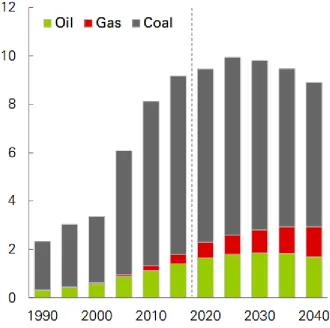
Annual, 2012]. According to the British Petroleum (BP) energy outlook in 2018 shown in Fig.
1.2, the world’s coal demand prediction remains stable from 2018, but still remains high and
ranks as the second largest energy source [British Petroleum Review of World Energy, 2018].
Figure 1.1 Primary energy regional consumption by fuel 2018 (Billion ton) (BP
Figure 1.2 Primary Fuel Demand in 2018 (Billion ton) (BP statistical review of world
energy)
Despite the importance of coal utilization, the combustion of these kinds of fossil fuel can
cause considerable environmental pollution. Raw coal contains certain amounts of impurities
such as mineral matter (gangue), ash and stone. Raw coal typically does not meet the
requirements for commercial application. For example, specific gasifier requires specific feed
coal size [Smith, 1981]. Furthermore, the impurities in raw coal such as gangue have low calorific
values. Meanwhile, the combustion of these impurities consume a lot of energy and release large
amounts of CO2, NOx, SOx, etc. At present, over 80% of CO2 and SO2 emission in air pollution
are from coal combustion. As shown in Fig. 1.3, coal combustion contributes to about 90% of the
of increasing calorific value by removing impurities from raw coal. This process can significantly
reduce the ash and gangue content of coal. More importantly, it allows raw coal to meet the final
standard by going through some production operations without changing its physical properties.
Coal beneficiation before combustion can greatly improve coal utilization efficiency and reduce
its environmental impact [Penner et al. 1987]. Therefore, coal cleaning technology is becoming
increasingly important.
Figure 1.3 Carbon emissions by source in 2018 (Billion tones CO
2) (BP statistical
review of world energy)
1.2
Bubbling fluidized bed applied in coal beneficiation
Fluidization is the phenomenon that particles show fluid-like behavior in the presence of an
upward flowing fluid. With different fluid velocities, the bed undergoes different fluidization
fluidization velocity. When inlet gas velocity reaches and exceeds the minimum fluidization
velocity, particles begin to fluidize and bubbles may form, leading to a bubbling fluidization
regime. The emulsion/dense phase is formed by the suspended dense granular particles and part
of the gas, while the bubble phase consists of bubbles only.
Bubbling fluidized bed have been used in many industrial processes due to its high mass and
heat transfer rates between gas and solid phases compared to fixed beds [Busciglo et al. 2012].
Chemical industries take great advantage of bubbling fluidized bed especially in coal separation
procedures.
Traditional coal beneficiation technology is divided into two categories: wet beneficiation
and dry beneficiation. Wet coal beneficiation needs large amounts of water. Considering the
global water shortage, the conventional wet coal separation method is greatly restricted. When
compared to the wet coal beneficiation, dry coal beneficiation, which is based on gas-solid
fluidized bed, has a lot of advantages such as saving process water, low moisture content after
beneficiation, lower environmental pollution and so on [Luo et al. 2008]. Therefore, dry coal
beneficiation is expected to replace the traditional wet coal beneficiation in the near future.
Dry coal beneficiation takes advantage of the gas-solid fluidized bed technology, using the
density difference between the bed medium and raw coal constituents to achieve the separation
[Luo & Chen, 2001]. The gas-solid fluidized bed has fluid-like characteristics, which allows
objects with higher density than the bed medium to sink to the bottom, while lighter objects float
on top of the bed [Luo & Chen, 2001; Dwari & Rao, 2007]. The density difference between raw
coal and the fluidized bed enables the separation process, which is a crucial factor in dry coal
beneficiation. The efficiency of the dry coal beneficiation can be controlled by controlling the
density of the fluidized bed. In industry applications, the fluidized bed density is usually
can only control the variation of the fluidized bed density in a small range and some useful
density ranges cannot be covered. Therefore, it is useful to introduce binary mixtures as the
fluidized medium because it can adjust separation density in a wider range [Douglas & Walsh,
1966]. The utilization of binary mixtures in dry coal beneficiation can realize the separation of
raw coal with a wider range of density and size. Furthermore, the uniformity of the bed density
throughout the whole fluidized bed which affects the separation efficiency also plays an
important role in the process. In the bubbling fluidized bed, the existence of bubbles is the most
significant factor that causes non-uniformity in bed density.
The Archimede’s principle explains the coal separation mechanism based on the forces
acting on the coal particles, as shown in Fig. 1.4.
Figure 1.4 Forces acting on a coal particle
Fd is the drag force caused by the rising bubble. Fb is the buoyant force caused by the
fluidized particles. Ff is the friction force caused by the interaction between the coal particle and
The existence of the bubble can reduce the friction force acting on coal particles. However,
ascending large bubble will drag particles in their wake, which can increase the drag force acting
on the coal particles and make the separation difficult. In order to maintain the bed density and
reduce the friction force and drag force, it is necessary to make sure the gas-solid fluidized bed
has small bubbles to maintain the bed density and reduce particles’ drag force.
1.3
Objectives
Because of the scarce amount of studies conducted on the behavior of mixtures of particles
in the fluidized beds, which have the same aerodynamic diameter, this research aims to study the
bubble characteristics of binary mixtures with the same aerodynamic diameter using digital image
analysis technology. In this work, minimum fluidization velocity, bubble diameter, bubble rise
velocity, bubble volume fraction and bed expansion were measured. A preliminary study on the
process of bubble coalescence and splitting is carried out. In addition, a new method of tracing
dense phase composition is applied and a new correlation of the estimation of bed density is
introduced. This research main objectives:
(1) Study of the effect of different binary mixtures on the relationship between total bed pressure
drop and superficial gas velocity.
(2) Study of the relationship between bubble size and excess gas velocity and distance above the
gas distributor.
(3) Investigation of the effect of sand volume fraction and excess gas velocity on bubble size in
different systems.
(4) Detailed study of the relationship between bubble rise velocity and bubble size, sand volume
fraction and distance above the gas distributor.
(5) Prediction of bubble volume fraction under different operation conditions.
(6) Study of bubble size and total bubble volume change during bubble coalescence and bubble
(7) Development of a new method to trace dense phase composition and a new correlation to
2
Literature review
2.1
Gas-solid fluidization technology applied in coal
beneficiation
Fluidization technology applied in dry coal beneficiation has been studied for about 40 years
[Beeckmans & Goransson, 1982]. Fraser and Yancy first applied gas-solid fluidization
technology in coal beneficiation using river sand as the bed medium [Fraser & Yancey, 1926].
However, the required coal separation density was slightly higher than the bed density caused by
sand fluidization, which caused a large amount of clean coal in the jetsam. Weintraub et.al used
magnetite as the heavy medium material and successfully separated coal from its impurities
[Weintraub et al. 1979]. Furthermore, it was pointed out that the dry coal beneficiation was a
complex system. The separation efficiency could be affected by many parameters such as particle
size distribution, inlet gas velocity, bubble size and bubble rise velocity and so on. Therefore, a
fluidized bed was developed using magnetite and river sand and their mixtures as the medium to
separate raw coal [Iohn, 1971]. The bed density formed by fluidization of magnetite ranges from
1.7g/cm3 to 2.2g/cm3, while that of sand fluidization ranges from 1.2g/cm3 to 1.4g/cm3. The bed
density of the fluidization mixture varies between 1.2-2.2g/cm3, which cover the intermediate
ranges of densities. Warren Spring laboratory invented a dry coal beneficiation equipment
combining an inclined vibratory trough and a fluidized bed [Douglas & Walsh, 1966]. A
counter-current fluidized bed (CCFC) system was developed to separate sand and carbon mixtures
[Beeckmans & Minh, 1977]. An upward fluidization system was developed, which could produce
a lighter overflow and a heavier underflow. This device saved energy effectively [Barari &
Sengupta, 1980]. An air-dense medium-fluidized bed (ADMFB) designed at the China University
of Mining and Technology in 1994 has been widely used due to its high efficiency.
Recently, many researches have focused on the improvement and fundamental principle of
separation performance and attempted to quantify the separator size range [Mohanta et al.2011].
The interdependencies among all parameters has been investigated which can affect the
separation performance. An empirical model was established, which could be used to predict
operation parameters to achieve the optimum performance [Mohanta et al. 2013]. An empirical
equation was derived to predict position of the coal particle in non-bubbling condition ADMFB
[Prusti et al. 2015]. Experiments were carried out to study the effect of narrow size range of the
dense medium (magnetite) on coal separation. It had been found that the finer magnetite powders
had lower minimum fluidization velocity and could expand the lower separation limit of the
ADMFB [Zhao et al. 2015].
2.2
Two phase theory
In order to simplify the fluidization model in bubbling fluidized bed, it is common to
consider the bed to be composed of two phases: bubble phase and dense phase [Davidson &
Harrison, 1963; Grace & Clift, 1974]. The two phase theory was proposed by Toomey, as shown
Figure 2.1 Diagram of two phase theory in fluidized bed [Han, 2017]
This theory considers that the apparent gas flow rate beyond the minimum fluidization form
the bubbles. The volume of the dilute phase can be estimated by equation 2.1.
𝐺𝑏 = (𝑢𝑔− 𝑢𝑚𝑓)𝐴 (2.1)
where 𝐺𝑏 is volumetric flow rate of the bubble phase.
This theory is frequently used for modeling purposes and calculation of the bubble volume
2.3
Particle segregation and minimum fluidization velocity
Minimum fluidization velocity is the apparent inlet gas velocity when particles in the
fluidized bed begin to fluidize. Minimum fluidization velocity is an important variables when
designing a fluidized bed [Coltters & Rivas, 2004; Chiba et al. 1979; Kunz, 1970/71].
Many correlations for predicting the minimum fluidization velocity of single particle systems
have been developed based on particle and gas properties, such as particle and gas density, and
particle diameter [Coltters & Rivas, 2004]. Wen and Yu developed a correlation to estimate the
minimum fluidization velocity of a single particle system, which is used in many researches due
to its adaptability [Wen & Yu, 1966].
The particle mixing and segregation degree can affect the fluidized bed properties. Katz first
study the particle size distribution in a binary fluidized bed [Katz, 1957]. In the fluidized bed, the
component that tends to float is called flotsam, while the component that tends to sink is known
as jetsam [Rowe et al. 1972]. The three mixing/ segregation states were defined in a fluidized bed
as shown in Fig. 2.2 [Chiba et al. 1979].
Figure 2.2 Typical mixing/segregation states. (a) Completely mixed, (b) completely
In addition, it has been found that three mixing/segregation states showed different relations
between the bed pressure drop and superficial gas velocity, as shown in Fig. 2.3 and an empirical
equation was proposed to estimate the minimum fluidization velocity under the conditions of
complete and partially fluidized beds [Chiba et al. 1979; Noda et al. 1986]. The minimum
fluidization velocity strongly depended on the particle mixing condition and an equation for the
estimation of minimum fluidization velocity was reported based on Wen and Yu’s equation,
correlated by a function of the ratios of particles density and size [Noda et al. 1986].
Figure 2.3 Effect of the mixing/segregation state on the relationship between bed
pressure drop and superficial gas velocity (idealized). (a) Completely mixed, (b)
Completely segregated. (c) Partial mixing [Chiba et al. 1979]
2.4
Bubble size
After the inlet gas reaches the minimum fluidization velocity, the excess gas will go into the
dilute phase to form bubbles. Bubbles form at the bottom and then ascend and finally burst at the
of the most important index in the fluidized bed since it can affect most of the properties of the
bed such as mass and heat transfer rate, bubble rising velocity and most importantly it can affect
the dry coal beneficiation efficiency [Hotio & Nonaka, 1987].
Bubble coalescence is the dominant factor for bubble size growth [Darton et al. 1977]. The
first empirical equation to estimate the bubble size was reported by Yasui and Johanson in 1958
based on light transmission between the probes submerged in the fluidized bed [Yasui &
Johanson, 1958]. Subsequently, a number of correlations for estimating bubble diameter have
been proposed. An equation was reported based on the bubble assemblage model, which was used
to design catalytic fluidized bed reactors [Kato & Wen, 1969]. Another equation was derived by
Geldart, which can predict the bubble diameter in a 3D fluidized bed from bubble diameter data
in a 2D fluidized bed [Geldart, 1970]. Geldart’s equation has become more and more important
since the two dimensional fluidized bed is widely used in studying bubble characteristics with
different fluid dynamics [Ma et al. 2016]. A semi-empirical equation was presented to predict the
effect of fluidized bed diameter on the bubble size [Mori & Wen, 1975]. Darton’s equation
reported in 1977 was the most widely used equation due to its adaptability to almost all
conditions [Darton, 1977].
Some typical correlations to estimate the bubble size are shown below.
• Kota and Wen: 𝐷𝐵 = 1.4𝜌𝑝𝑑𝑝( 𝑢
𝑢𝑚𝑓) ℎ + 𝐷0 (2.2)
where 𝐷0= ( 6𝐺
П)
0.4/𝑔0.2 (2.3)
• Geldart: (𝑑𝑏)3𝐷
(𝑑𝑏)2𝐷=
8П 3
𝑓2𝐷
𝑓3𝐷 (2.4)
where 𝑓2𝐷 can be calculated by equation 2.5.
𝑛3𝐷= 1.5 𝑛2𝐷2
𝑓2𝐷 (2.5)
• Mori & Wen: 𝐷𝐵𝑀−𝐷𝐵
𝐷𝐵𝑀−𝐷𝐵0 = exp(−
0.3ℎ
where 𝐷𝐵0= 0.347(
𝐴𝑡(𝑢0−𝑢𝑚𝑓)
𝑛𝑑 )
2/5 (2.7)
• Darton: 𝐷𝑒= 0.54(𝑢 − 𝑢𝑚𝑓) 0.4
(ℎ + 4√𝐴0)0.8/𝑔0.2 (2.8)
Two techniques have been employed to study bubble characteristics in fluidized beds:
intrusive techniques and non-intrusive techniques. Both techniques have been used to describe the
fluid dynamics for many decades [Rudisuli et al. 2012; Busciglio et al. 2010]. Interference of the
sensors in intrusive techniques disturbs the fluidized bed hydrodynamics [Busciglio et al. 2008].
Moreover, the simple probe can only measure the length of the bubble but not the diameter and it
is hard to discriminate the number of the bubbles passing through the probe [Busciglio et al.
2008; Rudisuli et al. 2012; van Ommen & Mudde, 2008]. In recent years, digital image analysis
technology (DIA) has been widely used in studying fluid dynamics [Busciglio et al. 2008]. DIA is
particularly suitable for the two-dimensional gas-solid fluidized bed because of the clear
boundary between the two phases [Salehi-Asl et al. 2018]. In addition, the video recordings
method can record the bubbles in slow-motion, which are too fast for visual observation [van
Ommen & Mudde, 2008]. Lim et al. were the first researchers who used DIA to present bubble
properties, including bubble size, shape factor and aspect ratio [Lim et al. 1990]. A
semi-empirical equation was developed to estimate average bubble size and average bubble rise
velocity using a CCD camera in 2D-bubbling fluidized bed [Hull et al. 1999]. The distribution of
the two important bubble characteristics (shape factor and aspect ratio) as a function of gas
velocity was investigated using DIA in a 2D-fluidized bed [Caicedo et al. 2003]. A method based
on DIA was developed to measure the bed expansion and segregation dynamics in dense gas-solid
fluidized beds. It was reported that this technology could trace bubbles and voidage waves as well
[Goldschmidt et al. 2003]. A new method using image processing toolbox of MATLAB was
developed to study the hydrodynamics of bubbles using a digital video camera. A better
development of the DIA technology and the 2D fluidized bed drive the incredible progress of
fluid dynamic research in fluidized beds.
2.5
Bubble rise velocity
Davidson and Harrison developed the most widely used equation to estimate bubble rise
velocity [Davidson & Harrison, 1963]. It was found that bubble rise velocity was affected by
bubble diameter and excess gas velocity. The bubble rise velocity was measured using a probe in
a large multi-tuyered fluidized bed under several excess gas velocities. It was found that the
bubble rise velocity was a linear function of the excess gas velocities [Whitehead et al. 1967].
The average local bubble rise velocity was measured in cylindrical fluidized beds with different
diameters by means of a miniaturized capacitance probe [Werther, 1974]. Two velocimetry
procedures were put forward to measure bubble rise velocity. The two procedures were based on
the Eulerian velocimetry technique (EVT) and the Lagrangian velocimetry technique (LVT). The
research result showed that both of the two methods could well be used in complex dynamics in
freely bubbling beds [Busciglio et al. 2008]. The effect of bed material on bubble rise velocity
had been studied in a three-dimensional fluidized bed using noninvasive ultrafast electron beam
X-ray tomography. It was found that the low density linear polyethylene (LLDPE) particle had
higher bubble rise velocity compared with the other particles used in that research [Verma et al.
2014]. A number of approaches were investigated to estimate the bubble rise velocity, including
using average solids concentration and grey scale value as input signal based on cross-correlation
technique, two-dimensional cross-correlation concept and detailed signal analysis method. The
cross-correlation method based on the average solids concentration and the detailed signal
analysis method were able to predict a more accurate bubble rise velocity [Li et al. 2018].
2.6
Binary fluidized bed
There are few researches done on bubble dynamics in a bed of mixtures of particles. Kage et
two kinds of particles of the same density but of different sizes using optical fiber probes. In
addition, a new method of determining the bubble diameter at any distance above the gas
distributor in the system of two kinds of particles was proposed [Kage et al. 1991]. Some
experiments were preformed focusing on the preliminary analysis of bubble dynamics, including
bubble diameter, bubble number and bubble rise velocity using DIA technology. Mixtures of
same density but with different sizes were used in the experiments [Busciglio et al. 2012]. This
research was a starting point and laid the foundation for future studies on the bubble dynamics of
binary mixtures in fluidized beds.
Mixture of particles can be divided into two categories: particles of same size but different
densities and particles of same density but different sizes. Han et al. investigated the effects of
both particle size and particle density on bubble dynamics. Particle with larger size and higher
density tend to form larger bubbles [Han, 2017]. However, it has been found that segregation
could occur in both particles of the same size but different densities and particles of same density
but different sizes systems [Chiba et al. 1980]. Complete segregation and partial segregation can
cause non-uniformity in bed density inside the fluidized bed. In the dry coal beneficiation
process, the uniformity of the bed density also plays an important role. The mixture of particles of
larger size but lower density and particles of smaller size but higher density can mixed more
evenly, which is beneficial for coal separation. In addition, by controlling their aerodynamic
3
Experimental set-up and methodology
3.1
Materials and operating conditions
Two groups of sand and magnetite mixtures with the same aerodynamics diameter and the
same size and two pure particles system were used in this experiments. The sand volume fractions
in the four mixtures were 30.5%, 54%, 72%, 87.5%, respectively. Experiments were carried out
under three different excess gas velocities (uex) 1.6cm/s, 4.3cm/s, 7.1cm/s with 0.6m fixed bed
height (H0). Particles were completely mixed before the experiments by high gas velocity.
Particles properties and operating conditions are shown in Tables. 3.1.
Table 3.1 Experimental Particles Properties
3.2
Image processing in bubble dynamics
After reaching steady state condition in the fluidized bed, the bubbles are recorded by a
video camera (Cannon Ti3) with a 29Hz video frequency. Each frame has 1088*1920 pixels.
Particle Type Particle size (um) Vol. Fraction of Sand Density(kg/m3) Geldart Type
Magnetite225-Sand225
Magnetite: 150-300um Volume average diameter: 225um
0% 4650
B
30.5% 4040
54% 3570
Sand: 150-300um Volume average diameter: 225um
72.5% 3200
87.5% 2900
100% 2650
Magnetite225-Sand304
Magnetite: 150-300um Volume average diameter: 225um
0% 4650
B/D
30.5% 4040
54% 3570
Sand: 255-355um Volume average diameter: 304um
72.5% 3200
87.5% 2900
The information an image can convey is expressed in grayscale [Jing & Zhu, 2012]. Each
pixel represents one grayscale value. The grayscale value of a certain image ranges from 0 to 255.
Zero (0) grayscale value means black, while 255 means white. Therefore, the image can be
transferred into grayscale matrix using the MATLAB program. Bubbles can be recognized due to
the different greyscale values between the bubble phase and the dense phase. To avoid noise
points caused by the nonuniform distribution of light and make the bubble part appear more
prominent, the fixed bed is established by a picture and subtracted by the fluidized bed picture.
The non-zero greyscale value portion displays the position at where the bubbles exist. The
specific calculation process is as follows:
(1) Obtain that 29 images per second, as shown in Fig. 3.1 (a) and transfer the images into a
grayscale matrix.
(2) Subtract grayscale values of fluidized bed images of different conditions from that of fixed
bed images. After subtraction, record the result in the matrix. Set a threshold value to exclude
noise points and output the matrix. The threshold value is ranging from 10 to 30 which is
determined by certain conditions. Subsequently, convert the greyscale matrix into black and
white binary pictures, as shown in Fig. 3.1 (b). The white part represents dilute phase
(bubble), while the black areas represent dense phase.
(3) Depict the bubble area as a circle of equal surface area using the ‘Regionprops’ software as
shown in Fig. 3.1 (c). The ‘Regionprops’ software can directly obtain the total number of
Figure 3.1 Image Processing Procedure (a) Original RGB Image (b) Black and
White Binary Image (c) Image with Circles
3.3
Image processing in tracing dense phase compositions
The fluidized bed is divided into five sections (12cm height) for tracing particles
compositions. Particle composition of each section was recorded by a camera (Cannon Ti3)
through continuous shooting. Six images were taken in each section and the images without
obvious bubbles were used to analyze the particle composition, as shown in Fig. 3.2. A small
piece was selected randomly in each image with a length-width ratio of 16:9. Because of the
different on color of magnetite particles and sand particles, the particles can be distinguished by
different greyscale values of each pixels in the image. Sand particles are yellow, which have
higher greyscale value, while magnetite particles are black, which have lower greyscale value. In
order to remove the non-uniformity resulting from the distraction and reflection of light and solve
the problem of uneven particle color, a histogram of the number of pixels versus greyscale value
shown in Fig. 3.3. Two peaks in Fig. 3.3 represent greyscale value distribution of sand and
magnetite, respectively. The black line represent the threshold. In Fig. 3.3, the left side of the
threshold is magnetite particles while the right part is sand particles. The specific calculation
process is as follows:
(1) Storaging the images without obvious bubbles and getting rid of the images with obvious
bubbles, as shown in Fig. 3.2(a) and (b). Increase contrast of the images without obvious
bubbles and randomly cut a part of it, as shown in Fig. 3.2(c)
(2) Transfer the small part into greyscale matrix with a size of 1920*1080. Output a histogram of
the number of pixels verses greyscale value and determine the threshold of the particular image,
as shown in Fig. 3.3
(3) Count the number of pixels of which greyscale value is lower than the threshold and the pixels
higher than the threshold. Sand and magnetite volume fraction can be calculated by Equation
(3.1) and (3.2).
Sandvolumefraction =𝑁𝑜.𝑃𝑖𝑥𝑒𝑙𝑠(𝐺𝑟𝑒𝑦𝑠𝑐𝑎𝑙𝑒𝑉𝑎𝑙𝑢𝑒>𝑇ℎ𝑟𝑒𝑠ℎ𝑜𝑙𝑑) 1920∗1080 (3.1)
Magnetitevolumefraction =𝑁𝑜.𝑃𝑖𝑥𝑒𝑙𝑠(𝐺𝑟𝑒𝑦𝑠𝑐𝑎𝑙𝑒𝑉𝑎𝑙𝑢𝑒<𝑇ℎ𝑟𝑒𝑠ℎ𝑜𝑙𝑑) 1920∗1080 (3.2)
Figure 3.2 Original RGB images in tracing particle composition. (a) Image without
Figure 3.3 Histogram of greyscale value distribution
3.4
Aerodynamic diameter
The aerodynamic diameter (𝑑𝑎) is an imaginary particle size used to study the motion of
particle. It is defined as the diameter of a unit dense spherical particle (𝜌0 = 1000𝑘𝑔/𝑚3) which
has the same terminal velocity of the actual particle when is performed in still air [DeCalo et al.
2004]. For different particles which have the same aerodynamic diameter, their terminal velocity
will be the same, which means they have the same degree of fluidization.
The terminal velocity of a particle can be calculated using the following equation 3.3:
𝑣𝑡 = √
4𝑔𝑑𝑝(𝜌𝑝−𝜌𝑓)
3𝐶𝐷𝜌𝑓 (3.3)
3.5
Minimum fluidization velocity
As the gas velocity increase through the particles in a fixed bed, the total bed pressure drop
increases and the particles enter a dynamic state. In this process, the relationship between the total
pressure drop and the superficial gas velocity is approximately linear, as shown in Fig. 3.4 [Jin et
al. 2001]. When the total pressure drop of the fluidized bed becomes equal to the particles weight
divided by the bed area, particles begin to fluidize. This inlet superficial gas velocity is called
minimum fluidization velocity (Umf), after which the total pressure drop remains almost constant,
while increasing inlet gas velocity result in the bed expansion [Jin et al. 2001].
In general the defluidization method is used to determine the minimum fluidization velocity
to avoid the hysteresis caused by the fluidization method.
Figure 3.4 The determination of minimum fluidization velocity using the
relationship between total pressure and superficial gas velocity
3.6
Bubble size
The discrimination of the bubble phase from the dense phase is based on the grayscale value
dense phase. The proper thresholding value is chosen from 10 to 30 in order to exclude the noise
point. The area of the bubble is defined as the number of pixels that form the bubble. The area
equivalent bubble diameter 𝐷𝑒 can be calculated by the following equation 3.4:
𝐷𝑒= 2√ 𝐴𝑏
П (3.4)
Each bubble is delineated as a circle with the same surface area of the bubble using the
‘Regionprops’ software. The vertical abscissa and ordinate of the bubble position is the centroid
of the bubble [Busciglio et al. 2008; Mudde et al. 1994].
3.7
Bubble rise velocity
Bubble rise velocity was measured using the LVT method as described below. This method
identifies and tracks the specific bubble. The process is as follows:
(1) The horizontal and vertical coordinates of the bubble centroid in the first image are recorded
as matrix L1 and L2, respectively.
(2) The horizontal and vertical coordinates of the bubble center of mass in the second image are
recorded as matrix R1 and R2, respectively.
(3) In the second image, the center of the bubble is compared with the first bubble in the first
image to get the bubble rising distance which is calculated by the following equation 3.5:
Distance = √(𝑥𝑖1− 𝑥𝑖2)2+ (𝑦𝑖1− 𝑦𝑖2)2 (3.5)
The distance is recorded in matrix F1.
(4) Finding the minimum value in matrix F1, which is the bubble rising distance in unit time. Use
the column number to find the corresponding bubble in the second image. Bubble rise
velocity is equal to bubble rise distance over time interval (Δt), as shown in equation 3.6.
𝑢𝑏 =
𝐷𝑖𝑠𝑡𝑎𝑛𝑐𝑒
∆𝑡 (3.6)
3.8
Bed expansion
Direct observation method is used in this research to measure the fluidized bed height. Six
pictures were taken to obtain the fixed bed height (H0) and the average fluidized bed height (He).
Bed expansion (e) is calculated by equation 3.7:
e =𝐻𝑒−𝐻0
𝐻0 (3.7)
3.9
Experimental apparatus
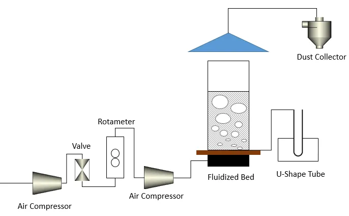
Fig.3.5 shows the schematic diagram of the 2D gas-solid fluidized bed. The fluidized bed
used to study the bubble dynamics is made of Perspex, which is consisted of a wind box, a
sintered plastic gas distributor, a 2D fluidized bed, an expanded section with a height of 1.12m
and a dust collector. The equipment without the expanded area is 1.5m high with a cross section
of 0.019m*0.37m. The gas distributor is made of sintered plastic material with holes of 10
microns. The air first goes into the wind box below the air distributor to ensure the uniform
distribution of the inlet gas across the bed and then goes through the gas distributor to fluidized
particles in the 2D fluidized bed. The fine particles blown away from the bed are collected in the
dust collector. The air flow rate is controlled by a rotameter (LZB-15) ranging from 0 L/h to 6000
L/h. A u-shape tube monometer is placed at the bottom of the bed to measure the total bed
pressure drop. Two lights (l-33, 500 WATTS) are placed on both sides of the front of the fluidized
bed to enhance the contrast between the bubble phase and dense phase in order to capture the
small bubbles and reduce the specular reflection, as shown in Fig. 3.6. The bubble behavior is
recorded by a Canon Ti3 camera directly in front of the fluidized bed, on the same side of the two
Figure 3.5 Schematic diagram of the bubbling fluidized bed
4
Result and discussion
4.1
Minimum fluidization velocity
Fig.4.1 and Fig.4.3 show the minimum fluidization velocities of two kinds of magnetite and
sand binary mixtures.
Figure 4.1 Determination of minimum fluidization velocities of binary mixtures
Figure 4.2 Segregation in the fluidized bed in Magnetite225-Sand225 system
Figure 4.3 Determination of minimum fluidization velocities of binary mixtures
The results from Fig.4.1 are in agreement with Chiba and Noda findings. When sand and
magnetite are of the same size, segregation appears in the system at a low gas velocity, as shown
in Fig.4.2, causing the three stages in the graph of pressure drop versus superficial gas velocity.
This is because magnetite is heavier than sand and would act as the jetsam, which tend to sink at
the bottom. Three velocities are able to clearly explain the three stages. The first inflection point
represents the initial fluidization velocity, meaning the lighter particles in the system have been
fluidized. After the initial fluidization velocity, particles with the higher minimum fluidization
velocity keep on moving until the superficial gas velocity reaches the second inflection point,
indicating the fluidization of the heavier particles. The minimum fluidization velocity is
determined at the intersection of the fixed bed and the horizontal line, which represents the
suspended state [Formisani et al. 2008]. However in Fig.4.3, the three stages phenomenon is not
obvious, which represents that particles with the same aerodynamic diameter mixed more evenly.
For the former two types of mixtures, the curves that fit minimum fluidization velocity,
initial fluidization velocity and complete fluidization velocity at varying sand volume fraction are
reported in Figs.4.4 and 4.5. Minimum fluidization velocity and initial fluidization velocity can
be reduced by adding lighter (sand) particles in the Magnetite225-Sand225 system. (Fig.4.4) In
the Magnetite225-Sand225 system, the complete fluidization velocity will decrease at high sand
volume fraction. This phenomenon has also been reported by B. Formisani [Formisani et al.
2008]. It seems that large amounts of lighter particles (sand) in the system make the binary
system behave more like a pure sand system. Ideally, the minimum fluidization velocities of
binary mixtures and pure particles in the Magnetite225-Sand304 system will be approximately
the same due to the same aerodynamic diameter they have. However, Fig. 4.5 shows that the
minimum fluidization velocities of binary mixtures have slightly decreased. This may be due to
the interaction between the sand and magnetite particles. Larger sand particles may wrap around
different conditions is very small, which also proves that when the aerodynamic diameter of sand
and magnetite are the same, their fluidization behavior is similar.
Figure 4.4 Minimum fluidization velocity, complete fluidization velocity and initial
fluidization velocity as a function of sand volume fraction in Magnetite225-Sand225
Figure 4.5 Minimum fluidization velocity as a function of sand volume fraction in
Magnetite225-Sand304 system
Many correlations have been developed for the estimation of minimum fluidization velocity,
for both single and binary particle systems. (Wen and Yu in 1966 for single particle and Noda et
al. in 1986 for binary particles [Wen & Yu, 1966; Noda et al. 1986].) Coltters and Rivas found a
strong dependency of particle properties such as particle shape and size distribution and particle
surface properties on minimum fluidization velocity [Coltters & Rivas, 2004].
The minimum fluidization velocity correlation for single particle system by Wen and Yu can
be described as follows:
𝐴𝑟 = 24.5𝑅𝑒𝑚𝑓2+ 1650𝑅𝑒𝑚𝑓 (4.1)
where
𝐴𝑟 = 𝑑3𝜌𝑔(𝜌𝑝− 𝜌𝑔) 𝑔
𝜇2 (4.2)
𝑅𝑒𝑚𝑓 =
𝑑𝜌𝑔𝑢𝑚𝑓
𝜇 (4.3)
Wen and Yu’s equation for a binary system. The average particle diameter and particle density of
binary mixtures are modified by the following equations in this study and applied in equation 4.1.
𝜌̅ = 𝜌𝑀𝑎𝑔𝑛𝑒𝑡𝑖𝑡𝑒𝑣𝑀𝑎𝑔𝑛𝑒𝑡𝑖𝑡𝑒+ 𝜌𝑆𝑎𝑛𝑑𝑣𝑆𝑎𝑛𝑑 (4.4)
𝑑̅ = √𝑑𝑀𝑎𝑔3𝑣𝑀𝑎𝑔𝑛𝑒𝑡𝑖𝑡𝑒+ 𝑑𝑆𝑎𝑛𝑑3𝑣𝑆𝑎𝑛𝑑
3
(4.5)
Noda rearranged equation 4.1 to 4.6, with average particle diameter and average particle
density defined as 4.4 and 4.5:
𝐴𝑟 = 𝐴𝑅𝑒𝑚𝑓
2+ 𝐵𝑅
𝑒𝑚𝑓 (4.6)
where A and B are constants:
A = 36.2(𝑑𝑃
𝑑𝐹
𝜌𝐹
𝜌𝑃)
−0.196 (4.7)
B = 1397(𝑑𝑃
𝑑𝐹
𝜌𝐹
𝜌𝑃)
0.296 (4.8)
A comparison between experimental minimum fluidization velocities and theoretical value is
Table 4.1 Comparison of minimum fluidization velocity
System Sands
Vol. Fraction (%)
Predicted Umf (m/s) Umf of this work (m/s)
Wen & Yu Noda Experimental
Magnetite225-Sand225
0 0.076 -- 0.099
30.5 0.067 0.089 0.094
54.0 0.059 0.079 0.082
72.5 0.053 0.071 0.072
87.5 0.048 0.065 0.061
100 0.044 -- 0.045
Magnetite225-Sand304
0 0.076 -- 0.099
30.5 0.084 0.077 0.096
54.0 0.086 0.078 0.093
72.5 0.084 0.077 0.097
87.5 0.082 0.075 0.098
100 0.079 -- 0.101
Table. 4.1 shows that Wen and Yu’s equation correlate well with the experimental result of
single particle system in both Magnetite225-Sand225 and Magnetite225-Sand304 systems.
Noda’s equation correlates better with the results of binary systems in the Magnetite225-Sand225
systems, which implies that particle properties have a great effect on the system and the
hydrodynamics of binary systems are different from single component systems. However, Wen
and Yu’s equation correlate better with the result of the binary mixtures in the
Magnetite225-Sand304 system. This may be due to the two particles of the same aerodynamic diameter having
4.2
Bubble size
4.2.1
Bubble size distribution
After the inlet gas reaches the minimum fluidization velocity, the excess gas will go into the
dilute phase to form bubbles. Bubbles form at the bottom and then ascend and burst at the bed
surface. Bubbles break up and coalesce continuously during this process [Horio & Nonaka,
1987]. Bubble coalescence is the dominant factor which leads to bubble size growth with the
distance above the gas distributor [Darton et al. 1977].
Bubble size distribution in axial and lateral position are shown in Fig. 4.6 and 4.7. From Fig.
4.6, it is obvious that bubble size increases with the increasing distance above the gas distributor.
Small bubbles disperse alongside the whole bed and the number of small bubble decrease with
the increasing distance above the gas distributor. Large bubbles appears at higher levels. The
sharp growth of bubble diameter at the distance of about 0.2m is mainly due to bubble
coalescence begin to happen at that level. At the distance of about 0.5m, bubble growth become
slower, which indicates that large bubble is harder to coalescence and the slightly increasing of
bubble size is mainly due to the decrease bed pressure drop with the increasing distance above the
gas distributor. From Fig. 4.7, the number of small bubbles at the edge of the fluidized bed is
larger than that in the center region. In addition, large bubbles tend to move to the middle of the
fluidized bed. This is because the chance of bubble coalescence is higher in the center region and
Figure 4.6 Bubble size distribution in axial position
Figure 4.7 Bubble size distribution in lateral position
4.2.2
Bubble size under different operating conditions
and Wen predicted a semi-empirical equation for bubble growth in fluidized beds for Geldart B
and Geldart D solids particles [Mori & Wen, 1975]. The equations are as follow:
𝐷𝐵𝑀−𝐷𝐵
𝐷𝐵𝑀−𝐷𝐵0= 𝑒 −0.3ℎ
𝐷𝑡 (4.9)
where 𝐷𝐵 is the diameter of the bubble, 𝐷𝑡 is the bed diameter, h is the height above the gas
distributor. The initial bubble diameter 𝐷𝐵0 for a porous plate is estimated using equation 4.10:
𝐷𝐵0= 0.00376(𝑢0− 𝑢𝑚𝑓)2 (4.10)
𝐷𝐵𝑀 is the limiting size of a bubble expected in a very deep fluidized bed and given by the
following equation:
𝐷𝐵𝑀= 0.652{𝐴𝑡(𝑢 − 𝑢𝑚𝑓)}0.4 (4.11)
where 𝐴𝑡 is the cross sectional area of the fluidized bed [Mori & Wen, 1975].
Darton’s equation is widely used due to its adaptability in most conditions [Darton et al.
1977]:
𝐷𝑒= 0.54𝑔−0.2(𝑢 − 𝑢𝑚𝑓)0.4(ℎ + 4𝐴𝐷0.5)0.8 (4.12)
where 𝐷𝑒 is the diameter of the sphere having the same volume of the bubble, U is the superficial
gas velocity and U = 𝑈𝑚𝑓 at the incipient fluidization, h is the distance above the gas distributor,
𝐴D is the ‘catchment area’ for the bubble stream at the gas distributor and is defined as the area of
each hole on the gas distributor.
Han et al. developed a new correlation which take bubble coalescence and splitting and
particle properties into consideration [Han, 2017]:
𝐷𝑒= ∅(𝑢 − 𝑢𝑚𝑓) 0.204
(ℎ + 4𝐴𝐷0.5) 0.759
/1.2 (4.13)
Ф= {
0.252(𝐹𝑜𝑟𝐺𝑒𝑙𝑑𝑎𝑟𝑡𝐵𝑡𝑦𝑝𝑒𝑜𝑓𝑝𝑎𝑟𝑡𝑖𝑐𝑙𝑒𝑠)
0.153(𝑓𝑜𝑟𝐺𝑒𝑑𝑎𝑟𝑡𝐴𝑡𝑦𝑝𝑒𝑜𝑓𝑝𝑎𝑟𝑡𝑖𝑐𝑙𝑒𝑠)
Figure 4.8 Average area equivalent bubble size as a function of distance above the
gas distributor under different excess gas velocity
gas distributor, which is due to the more frequent bubble coalescence at higher levels. Average
bubble size also increases with increasing excess gas velocity, as more gas will go to the dilute
phase and form bubbles. Bubble size grows faster at higher excess gas velocities. It may be due to
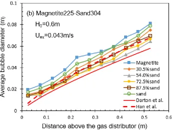
higher chance of coalescence at higher inlet gas flow rates. Fig. 4.9 shows the bubble size under
different sand volume fractions and the theoretical bubble size calculated by Darton’s equation
and Han’s equation. It is obvious that the bubble diameter calculated from Darton’s equation is
smaller than the experimental data. However the experiment shows a good correlation with the
bubble diameter calculated from Han’s equation. This result also indicates that bubble diameter is
affected by particle size and densities. In addition, bubble coalescence and splitting is another
crucial factor that may affect bubble diameter. Furthermore, Fig.4.9 also shows that bubble size
Figure 4.9 Average area equivalent bubble size of single-component particles and
4.2.3
Excess gas velocity, sands volume fraction and sand size
effects on bubble size
Fig. 4.10 shows the bubble size as a function of excess gas velocity at the same distance
above the gas distributor. It is evident that bubble size increases with increasing excess gas
velocity, which is in agreement with Fig. 4.8. Comparing with Fig. 4.10 (a), (b) and (c), a sharper
increase in bubble size can be observed at higher levels, which indicates more gas will move into
Figure 4.10 Average area equivalent bubble size as a function of excess gas velocity
Fig. 4.11 shows the effect of sand volume fraction on bubble diameter. Since the particles
flow characteristics in the Magnetite225-Sand304 system are very similar, the variation in sand
volume fraction can slightly affect the bubble diameter. In addition, adding lighter particles (sand)
into the system can reduce the bubble diameter. When the volume fraction of sand and magnetite
are identical, bubble diameter is at its smallest. This may be because that larger sand particles
wrap around the smaller magnetite particle, this process can not only reduce the particle density
but also mix the two particles more evenly. In addition, the minimum fluidization velocity of the
system with sand volume fraction of 54% is the smallest value, indicating that this system is
fluidized more easily compared to other systems and leads to the smallest bubble size. Larger
amounts of sand or magnetite particles in the system making the binary system behave more like
a pure particle system, which makes bubble size in these conditions to be closer to the pure
Figure 4.11 Average area equivalent bubble size as a function of sand volume
However, previous research shows that in the Magnetite225-Sand225 system, bubble size
will keep decreasing while adding light particles (sand) [Han, 2017]. When two particles of the
same size are in a system with decreasing amounts of sand, the bed density increases, which will
increase the downward force acting on the bubbles. Larger bubbles have larger surface area,
which can reduce the resistance acting on the bubble. This can cause the larger bubbles to ascend
more easily. However, in the Magnetite225-Sand304 system, when sand volume fraction is
higher, average particle size is larger while average particle density is lower. Both higher particle
density and larger particle size will form larger bubbles. In the Magnetite225-Sand304 system,
when sand volume fraction decreases to 54%, average particle diameter becomes smaller with the
decrease of sand while average particle density become higher with the increase of magnetite.
High amount of sane play a significant role in decreasing bubble size. When the sand amount
decreases from 54% to 0%, magnetite particles play a more dominant role. The increasing amount
of magnetite will lead to a higher average particle density, which leads to bubble size increase. In
addition, it has been found that when sand volume fraction decreases from 54% to 0%, the rate of
growth in bubble size first increases and then decreases. This may be due to the large amount of
magnetite compared to the amount of sand and adding sand will only have a slight effect on
bubble size. When sand exceeds a certain amount, the effect of sand on bubble size becomes
Figure 4.12 Average area equivalent bubble size as a function of excess gas velocity
in different systems
Fig. 4.12 shows the graph of bubble diameter against excess gas velocity in different
systems. It is obvious that in the Magnetite225-Sand304 system, gas velocity has a greater effect
on bubble diameter compared to the Magnetite255-Sand304 system. In the
Magnetite225-Sand304 system, sand and magnetite has similar fluidization behavior because of the same
aerodynamic diameter, and thus inlet gas velocity has little effect on the bubble size. While in the
Magnetite225-Sand225 system, magnetite begins to fluidize with an increasing gas velocity and
give rise to larger bubble diameter.
4.3
Bubble rise velocity
4.3.1
Bubble rise velocity under different operating conditions
A volume average bubble velocity is defined, which combines the bubble diameter with the𝑢𝑏=
∑𝑛𝑖=0𝑢𝑏𝑖𝑑𝐵𝑖2
∑𝑛𝑖=0𝑑𝐵𝑖2 (4.15)
In the 2-D fluidized bed, bubble is squeezed into a two dimensional state, so that the bubble
volume is proportional to𝑑𝐵2.
Figs. 4.13 and 4.14 illustrate that the volume average bubble rise velocity increases with the
distance above the gas distributor, and it is proportional to the excess gas velocity. In addition,
adding light particles (sand) can reduce the bubble rise velocity and this pattern completely
matches with the bubble size pattern. According to the bubble rise velocity equation of Davidson
and Harrison as shown below, bubble rise velocity is a function of bubble diameter and excess
gas velocity and the results are in agreement with the above conclusion [Davidson & Harrison,
1963].
Figure 4.13 Average bubble rise velocity as a function of distance above the gas
Figure 4.14 Average bubble rise velocities of single-component particle and binary
mixtures
4.3.2
Distance above the gas distributor and bubble size effect on
bubble rise velocity
Fig. 4.16 shows the effect of bubble size on bubble rise velocity in the same section. From Fig.
4.15, when the bubble size is small, bubble rise is approximately distributed in the same range
and remains unchanged alongside the whole bed. When bubble size increases, the bubble rise
velocity also increases. For bubble size larger than 6cm, bubble rise velocity disperse more
widely at higher levels. Fig. 4.16 clearly shows bubble rise velocity increases with the increasing
bubble size and it can also illustrate that the effect of height for the same bubble size is negligible.
These two Figures show that the increase in bubble rise velocity with respect to distance above
Figure 4.15 Bubble rise velocities of a single bubble with the same bubble diameter
Figure 4.16 The relationship between bubble rise velocity and corresponding area
equivalent bubble size in the same bed section
Fig. 4.17 shows the correlation between the bubble rise velocities and bubble diameter under
different excess gas velocities. The red line is the theoretical value calculated using equation 4.16.
This figure clearly shows that the experimental bubble rise velocities is in agreement with the
theoretical values. In addition, it also shows that the average bubble rise velocity is increasing
with the bubble diameter and the excess gas velocity. In the gas-solid fluidized system, bubble
rise velocity is affected by both buoyancy and friction from particles. Both larger bubble diameter
and higher gas velocity can reduce the resistance acting on the bubble, which leads to higher
Figure 4.17 Average bubble rise velocity as a function of average area equivalent
bubble size under different excess gas velocity and a comparison between
experimental data and theoretical value
4.3.3
Bubble volume fraction
In bubbling fluidization, the fluidized bed is divided into dense and bubble phases. The
apparent gas velocity in the fluidized bed which exceeds the minimum fluidization velocity will
form bubbles. The volumetric flow of bubble can be estimated using equation 4.17:
𝐺𝑏 = (𝑢𝑔− 𝑢𝑚𝑓)𝐴 (4.17)
where 𝐺𝑏 is the volumetric flow rate of bubble phase and A is the cross-sectional area of the
fluidized bed.
The volume of bubble phase in gas-solid bubbling fluidized bed is:
𝑑𝑉𝑏 = 𝐺𝑏 𝑑ℎ
𝑢𝑏 (4.18)


![Figure 2.1 Diagram of two phase theory in fluidized bed [Han, 2017]](https://thumb-us.123doks.com/thumbv2/123dok_us/1914531.1251054/23.612.147.529.83.354/figure-diagram-phase-theory-fluidized-bed-han.webp)