Theory of a Strip Antenna Located at the Interface of an Isotropic
Medium and a Magnetoplasma
Alexander V. Kudrin1, *, Anna S. Zaitseva1, Tatyana M. Zaboronkova1, 2, and Catherine Krafft3
Abstract—A study is made of the electrodynamic characteristics of an antenna having the form of a perfectly conducting, infinitesimally thin, narrow strip located at a plane interface of an isotropic medium and a cold collisionless magnetoplasma. The antenna is perpendicular to an external static magnetic field superimposed on the plasma medium and is excited by a time-harmonic given voltage. Singular integral equations for the antenna current are obtained in the case of an infinitely long strip conductor. Based on the solution of these equations, the current distribution and input impedance of the antenna are found for nonresonant and resonant frequency ranges of the magnetoplasma. The limits of applicability of an approximate approach employing the transmission line theory for determining the antenna characteristics are established. Within the framework of this approach, the results obtained are generalized to the case of a finite-length strip antenna.
1. INTRODUCTION
Electrodynamic characteristics of metal antennas in a magnetoplasma have been studied in many papers (see, e.g., [1–16] and references therein). The interest in the subject is stipulated by the wide use of such transmitters in various experiments in laboratory and space plasmas [17–22], and is stimulated continuously by the needs of practical applications such as diagnostics of plasma media, space communication, etc. In earlier theoretical works, antennas with given currents in a homogeneous magnetoplasma have been considered [1–7]. Such an approach is applicable to electrically small sources. For antennas with arbitrary sizes, the problem of finding the actual electromagnetic characteristics requires knowledge of the current distribution along the antenna wire. This problem, which turns out to be very difficult even for the simplest antennas operated in magnetized plasmas, has been solved only for some canonical antenna geometries [9–16]. Recently, increased attention has been paid to the features of excitation and propagation of electromagnetic waves in the presence of cylindrical magnetized plasma structures [23–26], and new results for loop antennas located on the surface of such structures have been obtained using the integral equation method [27, 28]. In particular, the current distribution and input impedance of a circular loop antenna located on the surface of an axially magnetized plasma column in a homogeneous dielectric medium have been found. It has been shown that the presence of a plasma column can lead to significant changes in the electrodynamic characteristics of the antenna compared with the cases of its operation in a homogeneous dielectric or plasma medium with the corresponding parameters.
Of no less interest is the problem of finding the characteristics of antennas located at a plane interface of a magnetoplasma and an isotropic medium. In particular, this problem is especially
Received 24 April 2018, Accepted 13 June 2018, Scheduled 22 June 2018
* Corresponding author: Alexander V. Kudrin ([email protected]).
topical for the development of plasma diagnostic methods that employ waves guided by planar dielectric structures in a plasma medium [29, 30]. Although an attempt has recently been made towards the theory of an antenna located at the interface of such media in [31], the analysis of that work is restricted to the special case of a rather dense resonant magnetoplasma, and is inapplicable for arbitrary plasma parameters. It is the purpose of this work to generalize the approach of [31] to the case where the magnetoplasma on one side of the interface between two media may have arbitrary parameters.
In this article, using the integral equation method, we solve a model problem of the current distribution and input impedance of a strip antenna that is perpendicular to an external static magnetic field and located at a plane interface of an isotropic medium and a cold collisionless magnetoplasma. We study the antenna characteristics in the cases of both a nonresonant and resonant magnetoplasma. Recall that the magnetoplasma is nonresonant if the diagonal elements of its dielectric tensor have identical signs, and is resonant otherwise [9–11]. As is known, the refractive index surfaces of the propagating normal waves of a nonresonant magnetoplasma are closed. On the contrary, for a resonant magnetoplasma, the refractive index of one of the normal waves goes to infinity at a certain angle between the wave vector and the direction of the external magnetic field [11]. It will be shown in what follows that the antenna characteristics are essentially different in these two cases.
Our article is organized as follows. In Section 2, we present the formulation of the problem. In Section 3, we describe the salient steps of the derivation of integral equations for the antenna current. Section 4 deals with the solution of these integral equations. In Section 5, we give analytical and numerical results for the electrodynamic characteristics of an infinitely long antenna and discuss generalization of these results to the case of a finite-length antenna. Section 6 presents conclusions following from the performed analysis.
2. FORMULATION OF THE PROBLEM
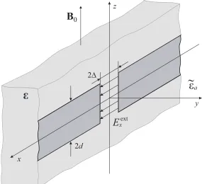
Consider an infinitely long antenna, which is oriented along thexaxis of a Cartesian coordinate system and has the form of a perfectly conducting, infinitesimally thin, narrow strip of width 2dlying in thexz
plane (see Figure 1). It is assumed that this plane coincides with the interface of a magnetoplasma and an isotropic medium. The external static magnetic field B0 is aligned with the z axis. The half-space
y <0 is filled with a homogeneous cold collisionless magnetoplasma, whose dielectric permittivity tensor has the form
ε=0
ε −ig 0
ig ε 0
0 0 η
, (1)
where 0 is the permittivity of free space. Expressions for the elements of the tensor in Equation (1)
are given elsewhere [32].
Homogeneous medium in the half-spacey >0 is isotropic and has a dielectric permittivity ˜εa=0εa. In the case where the medium in the region y >0 is free space, one should put εa= 1.
The current of the antenna is excited by a time-harmonic (∼exp(iωt)) given voltage that creates an electric field with the component Exext, which is nonzero for y = 0 and |z| < d in a narrow gap |x| ≤Δ:
Exext(x,0, z) = V0
2Δ[U(x+ Δ)−U(x−Δ)] [U(z+d)−U(z−d)]. (2) Here,V0 is the complex amplitude of the voltage applied to the gap, Δ is the gap half-width, and U is
a Heaviside function. The distribution of Exext for|z|< d can be represented by the Fourier integral
Exext(x,0, z) = k0 2π
∞
−∞V(nx) exp(−ik0nxx)dnx, (3)
where
V(nx) =V0
sin(k0nxΔ)
k0nxΔ
(4)
y z
x
a
E
xext2d
2Δ
B
0ε
∼
Figure 1. Geometry of the problem.
The density J of the electric current excited in the antenna by an external field that is given by Equation (3) can be sought in the form
J=x0I(x, z)δ(y), (5)
where |z| < d and δ(y) is a Dirac function. The surface density I(x, z) of the current admits the following representation:
I(x, z) = k0 2π
∞
−∞I(nx, z)exp(−ik0nxx)dnx. (6)
To find the distribution I(x, z), we express the tangential components Ex and Ez of the electric field excited by current (5) via the Fourier transform I(nx, z) of the surface current density and take into account boundary conditions for the field components at the interfacey = 0. In addition, we make use of boundary conditions for the tangential components of the electric field on the antenna surface (y= 0 and |z|< d):
Ex+Exext = 0, (7)
Ez = 0. (8)
The above-described procedure yields integral equations for the unknown quantity I(nx, z) and thus reduces the problem of determining the antenna current to the solution of the corresponding integral equations.
3. INTEGRAL EQUATIONS FOR THE ANTENNA CURRENT
Since the procedure of the derivation of integral equations for the antenna current was discussed in earlier work [31], we here describe only briefly the salient steps of this derivation and introduce notations that will be used in the further analysis generalizing the results of that work. We represent the antenna-excited field in the form
E(x, y, z)
H(x, y, z)
= k
2 0
(2π)2
∞
−∞
∞
−∞
E(nx, y, nz)
H(nx, y, nz)
It is a straightforward matter to show from the Maxwell equations that the quantities Ex,y(nx, y, nz) and Hx,y(nx, y, nz) can be expressed via the componentsEz(nx, y, nz) and Hz(nx, y, nz), which satisfy the following system of equations in the region y <0 [31]:
∂2Ez ∂y2 +k
2 0
η−n2x− η εn
2
z
Ez = −ik20g
εnzZ0Hz, (10) ∂2Hz
∂y2 +k 2 0
ε2−g2 ε −n
2
x−n2z
Hz = ik02g εηnzZ
−1
0 Ez, (11)
where Z0 is the impedance of free space. For the region y >0, one should put ε=η =εa and g = 0 in Equations (10) and (11). Solutions for the fields must satisfy the radiation condition at infinity (|y| → ∞), as well as the following boundary conditions for the tangential field components at the interfacey = 0:
Ex(nx, y−0, nz) =Ex(nx, y+ 0, nz), Ez(nx, y−0, nz) =Ez(nx, y+ 0, nz),
Hx(nx, y−0, nz) =Hx(nx, y+ 0, nz), Hz(nx, y−0, nz) =Hz(nx, y+ 0, nz)− I(nx, nz), (12)
where
I(nx, nz) = d
−d
I(nx, z) exp(ik0nzz)dz. (13)
It is seen from Equations (12) and (13) that the field components Ex, Ez, and Hx are continuous at the interface, whereas the component Hz is continuous at y = 0 for |z| > d and undergoes a jump corresponding to surface current (6) for |z|< d.
Upon solution of Equations (10) and (11), the Fourier-transformed tangential field components are written as
Ex(nx, y, nz) =i
2
k=1
Bkαknx+iny,k n2
⊥k
exp(ik0ny,ky),
Ez(nx, y, nz) =iη−1
2
k=1
Bknkexp(ik0ny,ky),
Hx(nx, y, nz) =Z0−1
2
k=1
Bknkβknx−iny,k n2
⊥k
exp(ik0ny,ky),
Hz(nx, y, nz) =−Z0−1
2
k=1
Bkexp(ik0ny,ky)
(14)
fory <0, and as
Ex(nx, y, nz) =− 1
n2
⊥
(C1nxnz+C2ny) exp(−ik0nyy),
Ez(nx, y, nz) =C1exp(−ik0nyy),
Hx(nx, y, nz) = 1
Z0n2⊥
(C1εany−C2nxnz) exp(−ik0nyy),
Hz(nx, y, nz) =Z0−1C2exp(−ik0nyy)
(15)
for y >0. Here, Bk and Ck are the coefficients determined using boundary conditions (12), while the other quantities are given by the formulas
n2⊥k = (2ε)−1
ε2−g2+εη−(η+ε)nz2+ (−1)k(η−ε)2n4z
+2(g2(η+ε)−ε(η−ε)2)n2z+ (ε2−g2−εη)21/2
nk= − ε
nzg
n2z+n2⊥k(nz) +g
2
ε −ε
, ny,k =n2⊥k(nz)−n2x1/2,
αk= n2z+n2⊥k(nz)−εg−1, βk=nznk−1, k= 1,2, n2⊥=εa−n2z, ny = (εa−n2x−n2z)1/2.
(16)
In order to ensure the fulfillment of the radiation condition at infinity, i.e., at|y| → ∞, the branches of the functionsny,k and ny in Equations (14) and (15) should be chosen so as to satisfy the inequalities Imny,k < 0 and Imny < 0. If the left-hand side of either of these inequalities vanishes, one should introduce a minor loss in the corresponding medium and, upon choosing the appropriate branch, go over to the limiting case of a loss-free medium.
After some algebra, we arrive at the following expressions for the tangential electric-field componentsEx(x, y, z) and Ez(x, y, z) at the interface y= 0:
Ex(x,0, z) = k0 2π
∞
−∞dnx
d
−d
Kx(nx, z−z)I(nx, z) exp(−ik0nxx)dz, (17)
Ez(x,0, z) = k0 2π
∞
−∞dnx
d
−d
Kz(nx, z−z)I(nx, z) exp(−ik0nxx)dz. (18)
Here,
Kx(nx, ζ) = iZ0k0 2π ∞ −∞ 2 k=1
ekB˜k
D exp(−ik0nz|ζ|)dnz, (19)
Kz(nx, ζ) = sgnζ iZ0k0
2πη ∞ −∞ 2 k=1
nkB˜k
D exp(−ik0nz|ζ|)dnz, (20)
whereζ =z−z. The coefficients ˜B1,2 and other quantities in Equations (19) and (20) are determined
by the expressions
˜
B1= −e2
η εa
nxnz n2⊥ +ih2
η εa
n2ny
n2⊥ −n2
εa−n2x εan2⊥ ,
˜
B2=e1
η εa
nxnz n2
⊥ −
ih1
η εa
n1ny
n2
⊥
+n1
εa−n2x εan2
⊥
,
D=n2
η
εae1h2+ iny
n2
⊥
(e1+
η εah2)
−n1
η
εae2h1+ iny
n2
⊥
(e2+
η εah1)
−(n2−n1)
εa−n2
x
εan2⊥ + η εa
nxnz
n2⊥ (e1+h1−e2−h2),
ek= αknx+iny,k
n2⊥k , hk=−
βknx−iny,k
n2⊥k , k= 1,2.
(21)
Since the tangential components of the electric field are continuous at the interface of a magnetoplasma and an isotropic medium, either the coefficientsBkor the coefficientsCkcan be used when deriving the expressions for these field components at y = 0. In Equations (19) and (20), we took the coefficients
Bk and made use of the fact thatBk=Z0B˜kI(nx, nz)/D.
From boundary conditions in Equations (7) and (8) for the tangential components of the electric field on the antenna surface with allowance for Equations (17)–(20), integral equations can be obtained for the Fourier transformI(nx, z) of the surface current density. From Equation (7), we have
d
−d
Kx(z−z)I(nx, z)dz =−V(nx). (22)
The boundary condition in Equation (8) gives d
−d
In integral Equations (22) and (23), it is assumed that |z|< d, and the integrals, which turn out to be singular forz−z→0, are understood in the sense of Cauchy’s principal value.
4. SOLUTION OF INTEGRAL EQUATIONS FOR THE ANTENNA CURRENT
The behavior of solutions of the integral equations for the antenna current is determined by the properties of their kernels in Equations (19) and (20). In what follows, we show that in the case of a fairly small antenna width 2d, where the inequalities
dΔ, d |η/ε|1/2Δ, (k0d)2max{|εa|,|ε|,|g|,|η|} 1 (24) are fulfilled, the properties of these kernels allow one to obtain an approximate solution of Equations (22) and (23) in closed form. To this end, we represent the kernels of these equations as the sums of singular and regular terms:
Kx(nx, ζ) =Kx(s)(nx, ζ) +Kx(r)(nx, ζ), Kz(nx, ζ) =Kz(s)(nx, ζ) +Kz(r)(nx, ζ),
where the quantities Kx(s)(nx, ζ) andKz(s)(nx, ζ) comprise singular terms that tend to infinity atζ →0, whereas the quantities Kx(r)(nx, ζ) andKz(r)(nx, ζ) remain finite (regular) in this limit. It can be shown that
Kx(s)(nx, ζ) = iZ0k0
π
βn2xεa ε2
a+|εη|
+ (1−β)n
2
x
εa+|εη|1/2sgnε−
1 2
∞
0
cos( k0nz|ζ|)
n2
z+n2x
dnz
+iβn
2
x|εη|1/2
ε2
a+|εη|
∞
α|nx|
cos(k0nz|ζ|)
n2
z−(αnx)2
dnz
, (25)
Kz(s)(nx, ζ) = Z0k0nx
π
βεa ε2
a+|εη|
+ 1−β
εa+|εη|1/2sgnε
∞
0
nzsin(k0nz|ζ|)
n2
z+n2x
dnz
+iβ|εη|
1/2
ε2
a+|εη|
∞
α|nx|
nzsin(k0nz|ζ|)
n2
z−(αnx)2
dnz
sgnζ. (26)
Hereafter, β= 0 if sgnε= sgnη,β = 1 if sgnε= sgn η, andα =|ε/η|1/2.
Formulas (25) and (26) can be derived by passing to the limit nz → ∞ in the integrands of Equations (19) and (20), respectively, with allowance for the identity
lim nz→∞
n2
z+n2x
nz − nz
n2
z+n2x
= 0. (27)
It can be verified that in the case where the half-space y <0 is filled with a resonant magnetoplasma, for which sgnε = sgnη, Equations (25) and (26) are reduced to the results of [31] if the plasma is sufficiently dense such that |εη| ε2
a. In contrast to [31], the representations in Equations (25) and (26) turn out to be valid for arbitrary plasma parameters, regardless of the signs and values ofεandη. The regular parts Kx(r)(nx, ζ) and Kz(r)(nx, ζ) of the kernels are found by subtracting the limiting quantities, which are obtained in the above-described way, from the corresponding integrands of Equations (19) and (20). We do not present very cumbersome formulas for Kx(r)(nx, ζ) andKz(r)(nx, ζ) here, because they are derived straightforwardly using the above explanations. Note that in the case of a narrow strip, i.e., under conditions in Equation (24), one can putζ = 0 when calculating the quantities
Kx(r)(nx, ζ) and Kz(r)(nx, ζ) in view of their regularity. In this case, the properties of the function
The integrals in Equations (25) and (26) can be evaluated analytically [33, 34] as follows:
∞
0
cos(k0nz|ζ|)
n2
z+n2x
dnz=K0(k0|nxζ|),
∞
α|nx|
cos(k0nz|ζ|)
n2
z−(αnx)2
dnz=−π
2Y0(k0α|nxζ|),
∞
0
nzsin(k0nz|ζ|)
n2
z+n2x
dnz=|nx|K1(k0|nxζ|),
∞
α|nx|
nzsin(k0nz|ζ|)
n2
z−(αnx)2
dnz=−π
2α|nx|Y1(k0α|nxζ|).
(28)
Here, Km and Ym are modified Bessel functions of the second kind and Bessel functions of the second kind of order m, respectively, and the evaluation of the last integral in Equation (28) was performed within the framework of the theory of tempered distributions. With allowance for the well-known small-argument approximations of cylindrical functions, in the limitζ →0 we have
Kx(s)(nx, ζ) = −iZ0k0 2πχ ln
k0|ζ|
2 + ln|nx|+γ+F
, (29)
Kz(s)(nx, ζ) = Z0 2πεeff
nx
ζ , (30)
where
χ= εeff
n2
x−εeff
, (31)
γ = 0.5772. . . is Euler’s constant, and the quantityF for sgnε= sgnη is defined as
F =iχn
2
x|εη|1/2
ε2
a+|εη| ln|ε|
|η|. (32)
In the opposite case where sgnε= sgnη, one should putF = 0. The quantityεeff is determined by the
expression
εeff =
εp+εa
2 , (33)
where
εp=
(εη)1/2sgnε if sgnε= sgnη,
−i|εη|1/2 if sgnε= sgnη. (34)
It should be noted that rigorously speaking, approximate expressions (29) and (30) cease to be valid for sufficiently large values of |nx|. However, as is evident from what follows, the |nx| values significantly exceeding (k0Δ)−1 affect only slightly the results of calculating the antenna current.
Hence, the fulfillment of the first two inequalities in Equation (24) ensures the applicability of the used approximations.
After the above algebra, integral Equations (22) and (23) are rewritten for|z|< das d
−d
I(nx, z) lnk0|z−z
|
2 dz
= −i2πχ
Z0k0
V(nx)−S(nx) d
−d
I(nx, z)dz, (35) d
−d
nxI(nx, z
)
z−z dz
= 0, (36)
where
The solution of Equation (35) with a logarithmic kernel, which also satisfies Equation (36) with Cauchy’s kernel [35], can be obtained in closed form as
I(nx, z) = 2i
Z0k0
√
d2−z2
χV0
ln(4/k0d)−S(nx)
sin(k0nxΔ)
k0nxΔ
. (38)
Substituting Equation (38) into Equation (6), we arrive at the formula for the surface current density
I(x, z). IntegratingI(x, z) overzfrom−dtodyields the total currentIΣ(x) of the antenna in the cross
section x= const:
IΣ(x) =
iV0
Z0
∞
−∞
sin(k0nxΔ)
k0nxΔ
χexp(−ik0nxx) ln(4/k0d)−S(nx)
dnx. (39)
Note that the singularity of the functionI(x, z) at|z| →d, which corresponds to the Meixner condition at the edge [36], turns out to be integrable, so that the total current of the antenna is finite.
5. CURRENT DISTRIBUTION AND INPUT IMPEDANCE OF THE ANTENNA
The integral representation in Equation (39) admits only a numerical study in the general case. However, if the condition ln(4/k0d) |S(nx)| holds for the values |nx| < (k0Δ)−1, which give the
main contribution to the integral in Equation (39), this integral can be evaluated analytically and the antenna current takes the following form for|x|>Δ:
IΣ(x) =
V0
Z0
k0εeff
h
π
ln(4/k0d)
exp(−ih|x|), (40)
where
h=k0ε1eff/2. (41)
In the case where the current-distribution constant h is complex-valued, it is assumed that Imh <0. An approximate representation of Equation (40) corresponds to the transmission line theory. Accordingly, the conditions under which this representation was derived determine the limits of applicability of this theory for a strip antenna located at the interface of the media considered. It is evident that if the magnetoplasma on one side of the interface y= 0 is nonresonant, i.e., sgnε= sgnη, and (εη)1/2sgnε+εa >0, then the current behavior is the same as that for an antenna in a homogeneous transparent medium with the dielectric permittivity εeff. However, in the case (εη)1/2sgnε+εa < 0, which is possible for the nonresonant magnetoplasma with ε < 0 andη <0, the quantity h turns out to be purely imaginary and the antenna current exponentially decays with distance from the excitation gap. If the magnetoplasma is resonant such that sgnε= sgnη, the quantityεeff and hence the
current-distribution constant h are complex, so that the current shape is characterized by spatial oscillations whose amplitude decays along the antenna conductor with distance from the antenna input.
Using the current distributionIΣ(x), we can find the input impedanceZ of the antenna using the
formula Z =V0/IΣ(Δ). Within the framework of the approximation in Equation (40) for the current
under the additional condition |h|Δ1, we obtain
Z = Z0
π k0
h ln
4
k0d
. (42)
It is important that the above results can be extended to the case of a finite-length antenna if we represent it as a transmission line of length 2L. Following the standard approach [15], one can find the current of such an antenna in the form
IΣ(x) =
I0
sin(hL)sin [h(L− |x|)], (43)
where |x|< L,I0 =IΣ(0) is the current at the antenna input, andh is determined by Equation (41).
The quantity I0 is found asI0 =V0/ZL, whereZL is the input impedance of the finite-length antenna. For the known current shape IΣ(x)/I0, the impedance ZL can be calculated using the induced EMF method [37]. In the case of an electrically short antenna where |h|L 1, Equation (43) yields a “triangular” distribution of current along the antenna conductor (|x|< L):
Since detailed calculations of the antenna characteristics for all possible cases would take up much space, we now dwell on the most interesting examples of the antenna-current behavior. Namely, we will discuss the distribution of the antenna current if the quantity h is purely imaginary or complex. We assume that the angular frequency ω is much higher than the lower hybrid frequency of a magnetoplasma [23]. In this case, we can neglect contribution of the ion motion to the elements of the plasma dielectric tensor in Equation (1) and represent them as follows [32]:
ε= 1 + ω
2
p
ωH2 −ω2, g=−
ωp2ωH
(ω2H−ω2)ω, η= 1−
ωp2
ω2, (45)
where ωH and ωp are the gyrofrequency and the plasma frequency of electrons, respectively. The calculations were performed for the plasma parameters corresponding to the laboratory conditions:
ωH = 3.5×10⁹s−1 (external static magnetic fieldB0 = 200 G) and 4×10¹⁰s−1≤ωp≤8×10¹⁰s−1(the plasma density varies in the interval between 5×1011cm−3 and 2×1012cm−3). The isotropic medium
in the regiony >0 is free space, i.e., εa= 1.
First, we consider the frequencyω= 5×10⁹s−1lying in the rangeωH < ω < ωp, for whichε <0 and
η <0. In this case, the magnetoplasma in the half-space y <0 is nonresonant and, moreover, εeff <0.
Figure 2 shows the snapshots of the distributions of the antenna current, normalized to its value atx= 0, along the infinitely long antenna at the indicated frequency for k0d= 1.67×10⁻³, Δ = 5d, and three
values of the plasma frequencyωp = 4×10¹⁰s−1 (εeff =−43.75), ωp = 5.64×10¹⁰s−1 (εeff =−88.5),
and ωp = 8×10¹⁰s−1 (εeff = −178.1), which correspond to dashed curves 1, 2 and 3, respectively.
Note that for the chosen parameters, the results of calculations by Equation (39) and approximate formula (40) coincide with graphical accuracy. This fact implies that the off-diagonal element g of the plasma dielectric tensor affects the current distribution only slightly. Indeed, this element contributes only to the regular parts of the kernels of integral equations for the antenna current. These parts are not taken into account within the framework of the transmission line theory. Hence, the results yielded by this theory can be obtained even easier, namely, by using the uniaxial tensor with g= 0 instead of general tensor (1). The exponential decay of current with distance from the antenna input is explained by the fact that the quantityhis purely imaginary in the case considered. The solid lines with respective labels in Figure 2, which correspond to the chosen values of the plasma density ωp, present the results of calculations by formula (43) for a finite antenna with the dimensionless half-lengthk0L= 0.33. This
value is marked by the vertical dash-dot line in the figure. Note that for solid curves 1, 2, and 3 in Figure 2, |Imh|L= 2.2,|Imh|L= 3.14, and|Imh|L= 4.45, respectively.
Figure 3 shows the current distributions of the antenna in the case of a resonant magnetoplasma where sgnε = sgnη at the frequency ω = 109s−1. In this case, k0d = 3.33 ×10⁻⁴. We used the
previous value of ωH, but put k0L = 0.167 for a finite-length antenna. Curves 1, 2, and 3, which are
plotted for the same plasma frequencies as those in Figure 2, correspond to εeff = 0.5−i2.37×102,
εeff = 0.5−i4.73×102, andεeff = 0.5−i9.45×102, respectively. Since the quantityεeff is now
complex-valued, the snapshots of the antenna current have oscillations that exponentially decay with distance from the antenna input.
It is seen in Figures 2 and 3 that the current distribution of the infinitely long antenna satisfactorily approximates the current behavior of the finite-length antenna for|Imh|L >3, excepting small regions near the endsz=±L. In this case, the input impedance of an infinitely long antenna can be used as a good approximation for the impedanceZL of the antenna of finite length. However, one should bear in mind that in the case of a purely imaginary h, the impedance given by Equation (42) has a zero real part. To determine ReZ, the regular part of kernel (19) must be taken into account. In contrast to this, in the case of a resonant magnetoplasma where h is complex, Equation (42) yields both the real and imaginary parts of the antenna impedance. This is due to the fact that the transmission line theory for a resonant magnetoplasma accounts for the excitation of quasielectrostatic waves in the plasma, which are known to predominantly determine the radiation resistance of a thin-wire antenna [3, 11, 16].
0 0.05 0.1 0.15 0.2 0.25 0.3 0.35 0
0.2 0.4 0.6 0.8 1
Re
[
(
)/
(0)]
Ix
I
k x
01
2
3
k L0
Σ
Σ
Figure 2. Current distributions along the infinitely long antenna (dashed lines) and the finite-length antenna (solid lines) for ω = 5×10⁹s−1 and ωH = 3.5×10⁹s−1 in the cases where ωp = 4×10¹⁰s−1 and |Imh|L= 2.2 (curves 1),ωp = 5.64×10¹⁰s−1 and |Imh|L= 3.14 (curves2), andωp = 8×10¹⁰s−1 and|Imh|L= 4.45 (curves 3). The vertical dash-dot line indicates thek0Lvalue on the horizontal axis.
0 0.02 0.04 0.06 0.08 0.1 0.12 0.14 0.16 0.18
-0.2 0 0.2 0.4 0.6 0.8 1
k x
0Re
[
(
)/
(0)]
Ix
I
1
2
3
k L0
ΣΣ
6. CONCLUSION
In this work, through the use of the theory of singular integral equations, we have considered the problem of finding the electrodynamic characteristics of a perfectly conducting, narrow strip antenna that is perpendicular to the external static magnetic field and located at a plane interface of a magnetoplasma and an isotropic medium. The cases of both a resonant and nonresonant plasma occupying the half-space on one side of the interface have been analyzed. For an infinitely long strip, we have obtained the current distribution and input impedance of such an antenna and established conditions under which these characteristics admit relatively simple closed-form representations corresponding to the transmission line theory. Within the framework of this theory, the current distribution and input impedance of the antenna coincide with the corresponding characteristics of a certain equivalent transmission line. We have also discussed the possibility to construct approximately the current distribution for a finite-length antenna. In the cases where the imaginary part of the current-distribution constant is nonzero and the antenna is not too short, the results obtained for an infinitely long antenna are shown to be applicable for a finite antenna.
Another important implication of the performed analysis is that the current-distribution constant derived within the framework of the transmission line theory turns out to be independent of the off-diagonal element of the plasma dielectric tensor. This fact allows one to employ the uniaxial model of a magnetoplasma when determining the antenna characteristics in a first approximation. A similar approach can evidently be used for finding the characteristics of an antenna located at an interface of more complex media described by permittivity or permeability tensors of arbitrary form.
ACKNOWLEDGMENT
The study of the current distribution of an infinitely long antenna was supported by the Russian Science Foundation (project No. 14-12-00510). Other results were obtained under support of the Ministry of Education and Science of the Russian Federation (project No. 3.1358.2017/4.6).
REFERENCES
1. Balmain, K. G., “The impedance of a short dipole antenna in a magnetoplasma,” IEEE Trans. Antennas Propagat., Vol. 12, No. 5, 605–617, 1964.
2. Lee, S. W. and Y. T. Lo, “Current distribution and input admittance of an infinite cylindrical antenna in anisotropic plasma,”IEEE Trans. Antennas Propagat., Vol. 15, No. 2, 244–252, 1967. 3. Wang, T. N. C. and T. F. Bell, “Radiation resistance of a short dipole immersed in a cold
magnetoionic medium,”Radio Sci., Vol. 4, No. 2, 167–177, 1969.
4. Wang, T. N. C. and T. F. Bell, “On VLF radiation resistance of an electric dipole in a cold magnetoplasma,” Radio Sci., Vol. 5, No. 3, 605–610, 1970.
5. Duff, G. L. and R. Mittra, “Loop impedance in magnetoplasma: Theory and experiment,” Radio Sci., Vol. 5, No. 1, 81–94, 1970.
6. Bell, T. F. and T. N. C. Wang, “Radiation resistance of a small filamentary loop antenna in a cold multicomponent magnetoplasma,”IEEE Trans. Antennas Propagat., Vol. 19, No. 4, 517–522, 1971.
7. Wang, T. N. C. and T. F. Bell, “VLF/ELF input impedance of an arbitrarily oriented loop antenna in a cold collisionless multicomponent magnetoplasma,” IEEE Trans. Antennas Propagat., Vol. 20, No. 3, 394–398, 1972.
8. Ohnuki, S., K. Sawaya, and S. Adachi, “Impedance of a large circular loop antenna in a magneto-plasma,”IEEE Trans. Antennas Propagat., Vol. 34, No. 8, 1024–1029, 1986.
9. Lee, S. W., “Cylindrical antenna in uniaxial resonant plasmas,”Radio Sci., Vol. 4, No. 2, 179–189, 1969.
11. Mareev, E. A. and Yu. V. Chugunov, Antennas in Plasmas, Institute of Applied Physics, Nizhny Novgorod, 1991 (in Russian).
12. Zaboronkova, T. M., A. V. Kudrin, and E. Yu. Petrov, “Toward the theory of a loop antenna in an anisotropic plasma,” Radiophys. Quantum Electron., Vol. 41, No. 3, 236–246, 1998.
13. Kudrin, A. V., E. Yu. Petrov, and T. M. Zaboronkova, “Current distribution and input impedance of a loop antenna in a cold magnetoplasma,”Journal of Electromagnetic Waves and Applications, Vol. 15, No. 3, 345–378, 2001.
14. Zaboronkova, T. M., A. V. Kudrin, and E. Yu. Petrov, “Current distribution on a cylindrical VLF antenna in a magnetoplasma,” Radiophys. Quantum Electron., Vol. 42, No. 8, 660–673, 1999. 15. Kudrin, A. V., E. Yu. Petrov, G. A. Kyriacou, and T. M. Zaboronkova, “Insulated cylindrical
antenna in a cold magnetoplasma,”Progress In Electromagnetics Research, Vol. 53, 135–166, 2005. 16. Zaboronkova, T. M., A. V. Kudrin, and E. Yu. Petrov, “Electrodynamic characteristics of a strip
antenna in a magnetoplasma,” J. Commun. Technol. Electron., Vol. 57, No. 3, 296–300, 2012. 17. Golubyatnikov, G. Yu., S. V. Egorov, A. V. Kostrov, E. A. Mareev, and Yu. V. Chugunov,
“Excitation of electrostatic and whistler waves by an antenna of magnetic type,”Sov. Phys. JETP, Vol. 67, No. 4, 717–723, 1988.
18. Kostrov, A. V., A. V. Kudrin, L. E. Kurina, G. A. Luchinin, A. A. Shaykin, and T. M. Zaboronkova, “Whistlers in thermally generated ducts with enhanced plasma density: Excitation and propagation,” Phys. Scr., Vol. 62, No. 1, 51–65, 2000.
19. Amatucci, W. E., D. D. Blackwell, D. N. Walker, G. Gatling, and G. Ganguli, “Whistler wave propagation and whistler wave antenna radiation resistance measurements,” IEEE Trans. Plasma Sci., Vol. 33, No. 2, 637–646, 2005.
20. James, H. G. and K. G. Balmain, “Guided electromagnetic waves observed on a conducting ionospheric tether,”Radio Sci., Vol. 36, No. 6, 1631–1644, 2001.
21. Chugunov, Yu. V. and G. A. Markov, “Active plasma antenna in the Earth’s ionosphere,”J. Atmos. Sol.-Terr. Phys., Vol. 63, No. 17, 1775–1787, 2001.
22. Shirokov, E. A., A. G. Demekhov, Yu. V. Chugunov, and A. V. Larchenko, “Effective length of a receiving antenna in case of quasi-electrostatic whistler mode waves: Application to spacecraft observations of chorus emissions,”Radio Sci., Vol. 52, No. 7, 884–895, 2017.
23. Helliwell, R. A.,Whistlers and Related Ionospheric Phenomena, Dover Publications, Mineola, 2006. 24. Starodubtsev, M. V., V. V. Nazarov, and A. V. Kostrov, “Laboratory study of nonlinear trapping of magnetized Langmuir waves inside a density depletion,”Phys. Rev. Lett., Vol. 98, No. 19, 195001, 2007.
25. Shirokov, E. A. and Yu. V. Chugunov, “Model of the dynamics of plasma-wave channels in magnetized plasmas,”Radiophys. Quantum Electron., Vol. 59, No. 1, 22–32, 2016.
26. Stenzel, R. L., “Whistler waves with angular momentum in space and laboratory plasmas and their counterparts in free space,” Adv. Phys. X, Vol. 1, No. 4, 687–710, 2016.
27. Kudrin, A. V., A. S. Zaitseva, T. M. Zaboronkova, C. Krafft, and G. A. Kyriacou, “Theory of a strip loop antenna located on the surface of an axially magnetized plasma column,” Progress In Electromagnetics Research B, Vol. 51, 221–246, 2013.
28. Kudrin, A. V., A. S. Zaitseva, T. M. Zaboronkova, and S. S. Zilitinkevich, “Current distribution and input impedance of a strip loop antenna located on the surface of a circular column filled with a resonant magnetoplasma,” Progress In Electromagnetics Research B, Vol. 55, 241–256, 2013. 29. Katin, I. V. and G. A. Markov, “Wave diagnostics of plasmas using a dielectric waveguide,”
Radiophys. Quantum Electron., Vol. 42, No. 3, 191–201, 1999.
30. Markov, G. A. and I. V. Khazanov, “Diagnostics of plasma oscillations by the field of surface waves guided by a dielectric waveguide,” Plasma Phys. Rep., Vol. 28, No. 4, 274–285, 2002.
32. Ginzburg, V. L., The Propagation of Electromagnetic Waves in Plasmas, 2nd edition, Pergamon Press, Oxford, 1970.
33. Gradshteyn, I. S. and I. M. Ryzhik,Tables of Integrals, Series, and Products, 7th edition, Academic Press, New York, 2007.
34. Erd´elyi, A., W. Magnus, F. Oberhettinger, and F. G. Tricomi, Tables of Integral Transforms (Bateman Manuscript Project), Vol. 1, McGraw-Hill, New York, 1954.
35. Vorovich V. V., V. M. Aleksandrov, and V. A. Babeshko, Nonclassical Mixed Problems in the Theory of Elasticity, Nauka, Moscow, 1974 (in Russian).
36. Meixner, J., “The behavior of electromagnetic fields at edges,” IEEE Trans. Antennas Propagat., Vol. 20, No. 4, 442–446, 1972.