Volume 2008, Article ID 275716,17pages doi:10.1155/2008/275716
Research Article
TSI Finders for Estimation of the Location of
an Interference Source Using an Ariborne Array
Dan Madurasinghe and Andrew Shaw
Electronic Warfare and Radar Division, Defence Science and Technology Organisation, P.O. Box 1500, Edinburgh, SA 5111, Australia
Correspondence should be addressed to Dan Madurasinghe,[email protected]
Received 15 November 2006; Revised 21 March 2007; Accepted 20 August 2007
Recommended by Douglas B. Williams
An algorithm based on space fast time adaptive processing to estimate the physical location of an interference source closely asso-ciated with a physical object and enhancing the detection performance against that object using a phased array radar is presented. Conventional direction finding techniques can estimate all the signals and their associated multipaths usually in a single spectrum. However, none of the techniques are currently able to identify direct path (source direction of interest) and its associated multipath individually. Without this knowledge, we are not in a position to achieve an estimation of the physical location of the interference source via ray tracing. The identification of the physical location of an interference source has become an important issue for some radar applications. The proposed technique identifies all the terrain bounced interference paths associated with the source of inter-est only (main lobe interferer). This is achieved via the introduction of a postprocessor known as the terrain scattered interference (TSI) finder.
Copyright © 2008 D. Madurasinghe and A. Shaw. This is an open access article distributed under the Creative Commons Attribution License, which permits unrestricted use, distribution, and reproduction in any medium, provided the original work is properly cited.
1. INTRODUCTION
The issue of source localization has been discussed in the lit-erature widely by mainly referring to the estimation of source powers, bearings, and associated multipaths. By sources we mean electromagnetic sources that emit random signals, which can be considered as interferers in communication or radar applications. Some of the conventional techniques that can be used to estimate the signal direction and its associated multipaths include MUSIC [1], spatially smoothed MUSIC [2,3], maximum likelihood methods (MLM) [4], and esti-mation of signal parameters via rotational invariance tech-nique (ESPIRIT) [5]. All these techniques use the array’s spa-tial covariance matrix to estimate the direction of arrivals (DOAs), some of which are direct emissions and others are multipath bounces offvarious objects including the ground or sea surface. For example, the MLM estimator is capable of estimating all the bearings and the associated multipaths. However, none of the techniques are able to identify each source and its associated multipaths when there are multiple sources and multipaths. If we are able to identify each source and its associated multipath, then we will be able to use the
ray tracing to locate the position of each offending source. In many applications, it is sufficient to estimate the direction of an interferer and place a null in the direction of the source to retain the performance of the system; however, there are a number of scenarios where the interference is closely associ-ated with an object that we wish to detect and characterize; in which case, we need to localize and suppress the interference and enhance our ability to detect and characterize the object of interest.
In this paper, we briefly discuss the available techniques for identifying the DOA of sources. The main body of the work concentrates on the application of the TSI finders for identifying the physical location of the source of interest. First, we study the TSI finder in detail for its processing gain properties, which has not been discussed earlier [6]. Fur-thermore, we introduce a new angle domain TSI finder that works in conjunction with the lag domain TSI finder as a postprocessor. These two processors can lead to the physical location of the source of interest.
Section 2formulates the multichannel radar model with several interference sources and Section 3briefly discusses some appropriate direction finding techniques including the recently introduced super gain beamformer (SGB) [7]. It is important to note that MUSIC and ESPRIT also present potential processing techniques applicable to this problem, but these methods consume considerably more computation power and require additional processing to extract all of the information of interest. The rest of the paper assumes the re-ceiver processing has clearly identified the direction of arrival of the offending source. Under this assumption, in Sections 4and5we introduce the TSI finder in the lag and angle do-mains and analyse them in detail.Section 6introduces the necessary formulas for estimating the location of the inter-ferer source using TSI.Section 7illustrates some simulated examples.
2. FORMULATION
Suppose anN-channel airborne radar whoseN×1 steering manifold is represented bys(ϕ,θ), where ϕis the azimuth angle and θ is the elevation angle, transmits a single pulse wheres(ϕ,θ)Hs(ϕ,θ) = N, and the superscriptH denotes the Hermitian transpose. For the range gater (r is also the fast time scale or an instant of sampling in fast time),N×1 measured signalx(r) can be written as
x(r)=j1(r)s
ϕ1,θ1
+j2(r)s
ϕ2,θ2
+ a1
m=1
β1,mj1
r−n1,m
sϕ1,m,θ1,m
+ a2
m=1
β2,mj2
r−n2,m
sϕ2,m,θ2,m
+ε, (1)
where j1(r), j2(r) represent a series of complex random
amplitudes corresponding to two far field sources, with the directions of arrival pairs, (ϕ1,θ1) and (ϕ2,θ2),
respec-tively. The third term represents the terrain scattered in-terference (TSI) paths of the first source with time lags (path lags)n1,1,n1,2,n1,3,. . .,n1,a1, the scattering coefficients |β1,m|
2
< 1,m = 1, 2,. . .,a1, and the associated direction
of arrival pairs (ϕ1,m,θ1,m) (m = 1, 2,. . .,a1). The fourth
term is the TSI from the second source with path delays n2,1,n2,2,n2,3,. . .,n2,a2, the scattering coefficients|β2,m|
2
<1, m = 1, 2,. . .,a2, and the associated direction of arrivals
(ϕ2,m,θ2,m) (m = 1, 2,. . .,a2). More sources and multiple
TSI paths from each source are accepted in general, but for the sake of brevity, we are restricting this paper to one of each, and εrepresents the N ×1 white noise component.
In this study, we consider the clutter-free case (in practice, this can be achieved in many ways, by exploiting a trans-mission silence, by using Doppler to suppress the clutter, or by shaping the transmit beam). Furthermore, we assume ρ2
k =E{|jk(r)|
2}
(k=1, 2,. . .) are the power levels of each source and|βk,m|
2
ρ2k (m=1, 2,. . .) represent the TSI power levels associated with each TSI path from the kth source, whereE{· · · }denotes the expectation operator over the fast time samples. Throughout the analysis we assume that we are interested only in the source powers (as offending sources) that are above the channel noise power, that is,Jk=ρ2k/σ2n> 1, k = 1, 2,. . .,E{εεH} = σ2
nIN, whereJk is the interferer source power to noise power ratio per channel,σ2
nis the white noise power present in any channel andIN is the unit iden-tity matrix. Without loss of generality, we use the notations1
ands2 to represents(ϕ1,θ1) ands(ϕ2,θ2), respectively, but
the steering vectors associated with TSI arrivals are repre-sented by two subscript notations1,m = s(ϕ1,m,θ1,m)(m =
1, 2,. . .,a1), s2,m = s(ϕ2,m,θ2,m)(m = 1, 2,. . .,a2), and so
forth. Furthermore, it is assumed thatE{jk(r+l)jk∗(r+m)} = ρ2
kδ(l−m) (k=1, 2,. . .), where∗denotes the complex con-jugate operation. This last assumption restricts the applica-tion of this theory to noise sources that are essentially con-tinuous over the period of examination.
In general, the first objective would be to identify the source directions of high significance to the radar systems performance, which are identified asJk=ρ2k/σ2n>1. Choices for estimating the direction of arrival using the array’s mea-sured spatial covariance matrix are diverse as discussed ear-lier. The most commonly used beamformer for estimating the number of sources and the power levels in a single spec-trum is the MPDR [8]. This approach optimizes the power output of the array subject to a linear constraint and is ap-plicable to arbitrary array geometries and achieves signal to noise gain ofNat the output, usingNsensors. Other compu-tationally intensive super resolution direction finding tech-niques such as the MUSIC, ESPRIT, or multidimensional op-timization techniques based on the MLM estimator are suit-able for locating the direction of arrival of signals, but require further postprocessing to estimate the source power levels.
This study proposes the recently introduced [7] superior version of the MPDR estimator to achieve an upper limit of N2processing gain in noise. Furthermore, the new estimator
is able to detect extremely weak signals if a large number of samples are available which is particularly applicable to air-borne radar.
3. DIRECTION OF ARRIVAL ESTIMATION
3.1. MPDR approach
The MPDR [1] power spectrum obtained by minimizing wH1Rxw1subject to the constraintw1Hs(ϕ,θ)=1 is given by
Pm(ϕ,θ)=w1(ϕ,θ)HRxw1(ϕ,θ)
=s(ϕ,θ)HR−1
x s(ϕ,θ) −1
,
where
w1(ϕ·θ)=
R−1
x s(ϕ,θ) s(ϕ,θ)HR−1
x s(ϕ,θ)
(3)
andRx=E{x(r)x(r)H}.
To understand the concept of the processing gain in noise, let us assume a single source in the direction (ϕ,θ) is present. In this case, we haveRx = ρ2
1s(ϕ1,θ1)s(ϕ1,θ1)H+
σ2
nIN. The inverse ofRxis
R−1
x = 1 σ2
n
IN−s
ϕ1,θ1
sϕ1,θ1
H
N+σ2
n/ρ21
. (4)
The MPDR power spectrum is given by
PM(ϕ,θ)= ρ
2 1N+σ2n ρ2
1
N2−sHs
1|2
/σ2
n+N
, (5)
wheres=s(ϕ,θ) ands1 =s(ϕ1,θ1). This can be rewritten
(noting that for (ϕ,θ)=/ (ϕ1,θ1),sHs1≈0) as
Pm(ϕ,θ)= ⎧ ⎪ ⎪ ⎪ ⎨ ⎪ ⎪ ⎪ ⎩
ρ2 1+
σ2
n
N for (ϕ,θ)=
ϕ1,θ1
,
σ2
n
N for (ϕ,θ)=/
ϕ1,θ1
.
(6)
The output signal to residual noise ratio (residual interfer-ence in the case of multiple sources) is
PM
ϕ1,θ1
PM
ϕ,θ(ϕ,θ)=/ (ϕ1,θ1) =ρ21N
σ2
n
+ 1≈Nρ21
σ2
n
(7)
which is approximatelyNtimes the input signal to interfer-ence plus noise ratio (SINRin).Note.(ϕ,θ)=/ (ϕ1,θ1) really
means that the value of (ϕ,θ) is not in the vicinity of the point (ϕ1,θ1) or any other source direction. This notation
will be used throughout this study as a way of indicating the averaged power output corresponding to a direction with no associated source power. This can be considered as the aver-aged output power due to the input noise.
This improvement factor (N) can generally be defined as the processing gain factor. In theory, the processing gain can take higher values as the number of sources increases. For example, ifP1represents the total input power due to other
sources, SINRin=ρ21/(σ2n+P1). If all of them are nulled while
maintainingwHs=1, then SINR
out ≈ρ21/(σ2out), whereσ2out
is the output noise power. This leads to the processing gain: SINRout/SINRin =G×INR, whereG=σ2n/σ2outis the
pro-cessing gain in noise (≈Nwhen a small number of interfer-ing sources are present), and INR=(σ2
n+P1)/σ2nis the total interference to noise at the input (≥1).
3.2. Super gain beam former (SGB)
Consider the SGB [7] spectrum|Ps(ϕ,θ)|where
Ps(ϕ,θ)= 1
N2
N
k=1
uH ks(ϕ,θ) rHks(ϕ,θ)−
1 uHkrk
. (8)
uk is anN×1 column vector of zeros except unit value at thekth position, andrkis thekth column ofR−1
x . For a sin-gle sourceRx =ρ2
1s(ϕ1,θ1)s(ϕ1,θ1)H+Rn. In order to gain
some insight in to the behaviour of (8), we break the uniform noise assumption and assume Rn = diag(σ21,σ22,. . .,σ2N) is the noise only spatial covariance matrix. The exact inver-sion of Rx is given by R−1
x = R−n1 −βRn−1s1sH1R−n1, where β = (Δ+ 1/ρ2
1)− 1
andΔ = Nj=1σ−j2. Furthermore rk = R−1
x uk=σ−k2(IN−βR−n1s1sH1)uk, and for (ϕ,θ)=(ϕ1,θ1) we
havesH
1R−n1s=ΔandsH1R−n1s≈0 whenever (ϕ,θ)=/ (ϕ1,θ1)
(in fact, when (ϕ,θ) point is furthest away from (ϕ1,θ1)).
Therefore, for a single source, assumingρ2
1=/ 0 we have
Ps(ϕ,θ)=
⎧ ⎪ ⎪ ⎪ ⎪ ⎪ ⎪ ⎨ ⎪ ⎪ ⎪ ⎪ ⎪ ⎪ ⎩
ρ2 1
N2
N
k=1
σ2
kΔ−1
ρ2 1Δ+1
ρ2
1Δ+1−ρ21/σ2k
for (ϕ,θ)=ϕ1,θ1
,
ρ2 1
N2
N
k=1
−1 ρ2
1Δ+1−ρ21/σ2k
for (ϕ,θ)=/ϕ1,θ1
. (9)
Now if we restore the uniform noise assumption,σ2k = σ2
n(k=1, 2,. . .,N), we have
Ps(ϕ,θ)=
⎧ ⎪ ⎪ ⎪ ⎨ ⎪ ⎪ ⎪ ⎩
ρ2 1+
σ2
n
G for (ϕ,θ)=
ϕ1,θ1
,
−σ2n
G for (ϕ,θ)=/
ϕ1,θ1
,
(10)
whereG=N(N−1) +Nσ2
n/ρ21≈N2is the processing gain of
|Ps(ϕ,θ)|. This also suggests that for extremely weak signals, that is, as p→0, the processing gain tends to infinity [7]. In fact this is not the case, and the gain will be determined by the number of samples averaged to produce the covariance ma-trix. The SGB estimator is clearly able to identify the source signals as well as weak TSI signals in a single spectrum with a very clear margin as discussed in [7]. The price to pay to get a very low output noise level is a large sample support (>10N) for SGB. The angular resolution is only slightly better than the MPDR solution. The main advantage of SGB spectrum is its very low output noise floor level which enables us to de-tect weak signals. Attempting to apply higher processing gain algorithms, such as SGB(N3) would require more than 100N
sample support and this would not be practical for radar ap-plications. Hence, direction finding is a matured area and the intention of this section is to highlight the fact that it is not possible to relate each source with its associated TSI path us-ing available techniques. This task will be carried out usus-ing the TSI finders.
4. TSI FINDER (LAG DOMAIN)
use of the TSI path in this study is to locate the noise source. The array’sN×Nspatial covariance matrix has the follow-ing structure (for the case where two sources and one TSI off each source is present):
Rx=ρ2
1s1sH1 +ρ22s2sH2 +ρ21β1,1 2
s1,1sH1,1
+ρ2 2β2,1
2
s2,1sH2,1+σ2nIN.
(11)
Suppose now we compute the space fast time covariance R2of size 2N×2N corresponding to an arbitrarily chosen
fast time lagn; then we have
R2=E
Xn(r)Xn(r)H=
Rx ON×N ON×N Rx
forn /=n1,morn2,mm=1, 2,. . .,
(12)
whereXn(r)= (x(r)T,x(r+n)T)T is termed as the 2N×1 space fast time snapshot for the selected lagnandON×Nis the N×Nmatrix with zero entries. However, ifn=n1,morn2,m for somem, then we have (sayn=n1,1as an example)
Xn1(r)=
x(r) xr+n1,1
=j1(r)
s1
β1,1s1,1
+j2(r)
s2
oN×1
+β1,1j1
r−n1,1
s1,1
oN×1
+β2,1j2
r−n2,1
s2,1
oN×1
+j1
r+n1,1
oN×1
s1
+j2
r+n1,1
oN×1
s2
+β2,1j2
r−n2,1+n1,1
oN×1
s2,1
+
ε1
ε2
,
(13)
whereε1andε2represent two independent measurements of
the white noise component, andoN×1is theN×1 column
of zeros. In this case, the space fast time covariance matrix is given by
R2=
Rx QH
Q Rx
, (14)
whereQ=ρ2β
1,1s1,1sH1.
It is important to note that we assumen1,m (m=1, 2,. . .) represent digitized sample values of the fast time variabler and the reflected path is an integer valued delay of the di-rect path. If this assumption is not satisfied, one would not achieve a perfect decorrelation, resulting in a nonzero off di-agonal term in (12). In other words, a clear distinction be-tween (12) and (14) will not be possible. The existence of the delayed value of the termQcan be made equal to zero or not be suitably choosing a delay value forn1,1when forming the
space time covariance matrix. However,Qis a matrix and, as a result one may tend to consider its determinant value in order to differentiate the two cases in (12) and (14). After extensive analysis, one may find the signal processing gain
is not acceptable for this choice. More physically meaningful measure would be to consider its contribution to the overall processor output power (when minimized with respect to the look direction constraint). Depending on whether the power contribution is zero or not, we have the situation described in (12) or (14) clearly identified under the above assump-tions. Therefore, the scaled measure was introduced as the TSI finder [6], which is a function of the chosen delay value, nmust represent the scaled version of the contribution due to the presence ofQat the total output power. Even thought one can come up with many variations of the TSI finder based on the same principle, one expressed in this study is tested and verified to have high signal processing gain as seen later. Now suppose the direction of arrival of the interference source to be (ϕ1,θ1), the first objective is to find all its associated path
delays, which may be of low power and may not have been identified by the usual direction finders. This is carried out by the TSI finder in the lag domain by searching over all pos-sible lag values while the look direction is fixed at the desired source direction (ϕ1,θ1). This is given by the spectrum
Ts(n)=
1 Pout
sH
1R−x1s1
−1
, (15)
where Pout = wHR2w, w is the 2N ×1 space fast time
weights vector which minimizes the power while looking into the direction of the source of interest subject to the con-straints:wHsA =1 andwHsB =0, wheresA =(sT
1,oTN×1)
T , sB = (oT
N×1,sT1)
T
. The solutionw for each lag is given by w=λR−1
2 sA+μR2−1sBwhere the parametersλandμare given
by (one may apply Lagrange multiplier technique and opti-mize the functionΦ(w)=wHR
2w+β(wHsA−1) +ρwHsB
with respect tow, whereβ,ρare arbitrary parameters, as a result,∂Φ/∂w=0 gives usw=λR2−1sA+μR−21sB)
⎛
⎝sHAR−21sA sHBR−21sA
sH
AR−21sB sHBR2−1sB
⎞ ⎠
λ∗ μ∗
=
1 0
. (16)
As the search functionTs(n) scans through all potential lag values, one is able to identify the points at which a corre-sponding delayed version of the look direction signal is en-countered as seen in the next section.
DenotingRx=ρ2
1s1sH1 +R1, we have
R1=ρ22s2sH2 +β1,1 2
ρ21s1,1sH1,1+β2,1 2
ρ22s2,1sH2,1+σ2nIN. (17)
4.1. Analysis of the TSI finder
Now, for the sake of convenience, we represent the 2N×1 space fast time weights vector aswT =(wT
1,w2T)
T
, where the N×1 vectorw1refers to the firstN components ofw and
the rest is represented by theN×1 vectorw2. First suppose
the chosen lagnis not equal to any of the values n1,j(j = 1, 2,. . .). In this case, substituting (12) and (17) inPout =
wHR
2wwe have
Pout=w1HR1w1+wH2R1w2+ρ21wH1s1sH1w1+ρ12wH2s1sH1w2.
The minimization of power subject to the same constraints, wHsA = 1 andwHsB = 0 (i.e.,wH
1s1 = 1 andwH2s1 = 0),
leads to the following solution:
w1= R
−1
1 s1
sH
1R−11s1
, w2=oN×1. (19)
In this case, we have the following expression for the space fast time processor output power:
Pout=wHR2w=wH1R1w1+ρ21wH1s1sH1w1=
sH1R−1
1 s1
−1
+ρ2 1.
(20)
Substituting this expression into (15) leads to
Ts(n)n /=nk=
sH1R−x1s1
−1
sH1R−11s1
−1
+ρ2 1
−1≡0 (21)
(see Appendix A for a proof of the result (sH
1R−x1s1)
−1
=
(sH1R−11s1)− 1
+ρ2
1). It was noticed thatw2=0N×1if and only if
Q=0N×N. As a result, we would consider the scaled quantity (Pout−w1HR1w1−ρ21wH1s1sH1w1)/Poutwhich is a function ofw2
only as a suitable TSI finder. Simplification of this quantity using the look direction constraints together with the results inAppendix Aand (19) leads to (15).
The most important fact here is that we do not have to assume the simple case of a main lobe interferer and one TSI path to prove that this quantity is zero. The TSI finder spec-trum has the following properties, as we look into the direc-tion (ϕ1,θ1):
Ts(n)≈ ⎧ ⎨ ⎩P
−1
out
sH1R−x1s1
−1
−1, n=n1,j for some j,
0, n /=n1,j.
(22)
The TSI estimator indicates infinite processing gain when in-verted (at least in theory), and is able to detect extremely small TSI power. In the next section we would like to further investigate the properties of the estimator and its processing gain.
The output power at the processorPout(forn=n1,1) is
given by (using (14))
Pout=wHR2w=w1HR1w1+wH2R1w2
+ρ2w1Hs1sH1w1+ρ21wH2s1sH1w2
+ρ2 1β
∗
1,1wH1s1sH1,1w2+ρ12β1,1wH2s1,1sH1w1.
(23)
When the constraintswH
1s1 =1 andwH2s1=0 are imposed,
we have
Pout=wHR2w=wH1R1w1+wH2R1w2
+ρ2 1+ρ21
β∗1,1sH
1,1w2+β1,1wH2s1,1
. (24)
The original power minimization problem can now be broken into two independent minimization problems as
fol-lows.
(1) MinimizewH
1R1w1subject to the constraintw1Hs1=1.
(2) Minimize wH
2R1w2+ρ21+ρ21(β
∗
1,1sH1,1w2+β1,1wH2s1,1)
subject towH
2s1=0.
The solution can be expressed as
w1=
R−1 1 s1
sH1R1−1s1
, (25)
w2= −β1,1ρ21R1−1s1,1+β1,1ρ21
sH
1R−11s1,1
sH1R−11s1
R−11s1. (26)
The above representation of the solution cannot be used to compute the space-time weights vectorwdue to the fact that the quantities involved are not measurable. Instead, the re-sult in (16) is implemented to evaluatewas described in the previous section.
SubstitutingR1=ρ22s2sH2+ρ21|β1,1| 2s
1,1sH1,1+ρ22|β2,1| 2s
2,1sH2,1+
σ2
nIN into (24) and noting thatρ21|β1,1| 2
wH
2s1,1sH1,1w2+ρ21+
ρ2 1(β
∗
1,1sH1,1w2+β1,1wH2s1,1)=ρ21|1 +β1,1w2Hs1,1| 2
, we have the following expression for the output power:
Pout=ρ21β1,1 2
wH
1s1,1 2
+ρ2
11 +β1,1w2Hs1,1 2
+wH1R0w1+w2HR0w2+σ2n
wH1w1+w2Hw2
, (27)
whereR0=ρ22s2sH2 +|β2| 2
ρ2
2s2,1sH2,1is the output energy due
to any second source and associated multipaths present at the input. It should be noted that this component of the output also contains any output energy due to any second (unmatched) multipath of the look direction source (e.g.,
|β1,2| 2
s1,2sH1,2terms). The most general form would be
R0=
a1
j=2
ρ2 1β1,j
2
s1,jsH1,j+ q
k=2
ρ2
ksks2k
+ q
k=2
ak
j=1
ρ2
kβk,j
2
sk,jsHk,j,
(28)
whereqis the number of sources, andakis the number of TSI paths available for thekth source. The expression forPoutin
(27) clearly indicates that the bestw1that (which hasN
de-grees of freedom) would minimizePoutis likely to be
orthog-onal tos1,1, that is,|wHs1,1| ≈ 0, and furthermore it would
be attempting to satisfy|1 +β1,1wH
2s1,1|2≈0 while being
or-thogonal to all other signals present inR0.
Note that
wH
1R0w1=
a1
j=2
ρ2 1β1,j
2
wH
1s1,j2+ q
k=2
ρ2
kwH1sk 2
+ q
k=2
ak
j=1
ρ2
kβk,j
2
wH
1sk,j2
(29)
and a similar expression holds forwH2Rw2.
assume we have only a look direction signal and its TSI path, in which case we haveR0=ON×Nand
Pout=ρ21β1,1 2
wH1s1,1 2
+ρ211 +β1,1wH2s1,1 2
+σ2
n
wH1w1+wH2w2
. (30)
In this case,R1 = |β1,1|2ρ21s1,1sH1,1+σ2nIN and the inverse of which is is given by
R−11=
1 σ2 n IN− ρ2
1β1,1 2
s1,1sH1,1
σ2
n+Nβ1,1 2 ρ2 1 . (31)
As a result, we have
R−1 1 s1= 1
σ2
n
s1−
ρ2
1β1,1 2
s1,1sH1,1s1
σ2
n+Nβ1,1 2
ρ21
, (32)
R−1 1 s1,1=
s1,1
σ2
n+Nβ1,1 2
ρ2 1
, (33)
sH1,1R−11s1,1= N
σ2
n+Nβ1,1 2
ρ2 1
, (34)
sH
1,1R−11s1=
sH1,1s1
σ2
n+Nβ1,1 2
ρ21
. (35)
Furthermore, we adopt the notationJ1 =Jfor the look
di-rection interferer to noise power and (forN|β1,1|2J1)
sH1R−11s1=
1 σ2 n N− ρ2
1β1,1 2
sH1s1,1 2
σ2
n+Nβ1,1 2 ρ2 1 = N σ2 n
1− s
H
1s1,1 2
β1,12J
N1 +Nβ1,12J
≈ N
σ2
n
1−sH1s1,1 2 N2 ≈ N σ2 n . (36)
The assumption made in the last expression (i.e.,
|sH1s1,1| 2
/N2 ≈ 0) is very accurate when the signals are not
closely spaced. This assumption cannot be verified analyti-cally, it depends on the structure of the array, however, it can be numerically verified for a commonly used linear equis-paced array with half wavelength spacing. The other assump-tion made throughout this study is that the look direcassump-tion in-terferer is above the noise floor (i.e.,J>1). In this case, we need at least|β1,1|2
1/N (or equivalentlyN|β1,1|2J
1) in order to detect any TSI power as seen later. We will also see that when|β1,1|2
is closer to the lower bound of 1/N we do not achieve good processing gain to detect TSI unlessJis extremely large (but this case is not presented here).
Now, we would like to investigate the two cases|β1,1| 2
1/Nand|β1,1|2
1/Nsimultaneously.
The value of the expression (36) for|β1,1|21/Ncan be
simplified as follows:
sH
1R−11s1≈ N
σ2
n
1−s
H
1s1,1 2
β1,12J
N ≈ N σ2 n
1−s
H
1s1,12
Nβ1,12J
N2 ≈ N σ2 n . (37)
Throughout the study, this case is taken to be equivalent to N|β1,1|2J
1 as well, becauseJis not assumed to take ex-cessively large values for|β1,1|21/N. The investigation of
the signal processing gain for the case where|β1,1|2
1/N and at the same timeJis very large is outside of the scope of this study.
Furthermore, applying the above formula and (33) in (25), we can see that
wH
1s1,1 2
=sH1R−11s1,1
sH1R−11s1
2
= sH1
sH1R−11s1·
s1,1
σ2
n+Nβ1,1 2
ρ2 1
2
≈ sH1s1,1 2
/N2
1 +Nβ1,12J2 ≈0.
(38)
This expression shows how closely we have achieved the orthogonality requirement expected above. It is reasonable to assume thatwH
1s1,1≈0 (or equivalently|sH1s1,1| 2
/N2≈0)
for all possible positive values ofN|β1,1|2
. We may now in-vestigate the second and third terms as the dominant terms at the processor output in (30). The approximate expres-sions for these two terms can be derived using (32)–(36) (see Appendix B) as
1 +β
1,1wH2s1,1 2 ≈ ⎧ ⎪ ⎪ ⎨ ⎪ ⎪ ⎩ 1
Nβ1,12J2 forNβ1,1 2
J1,
1−2Nβ1,1 2
J forNβ1,1
2
J1,
σ2n w 2= ⎧ ⎪ ⎪ ⎪ ⎨ ⎪ ⎪ ⎪ ⎩ σ2 n 1 N+ 1 Nβ1,12
forNβ1,12J1, σ2
n
1
N +Nβ1,1 2
J2
forNβ1,1 2
J1.
(39)
Substituting (39) in (30), we can evaluatePout/σ2nas
Pout σ2 n = ⎧ ⎪ ⎪ ⎪ ⎪ ⎪ ⎪ ⎪ ⎪ ⎨ ⎪ ⎪ ⎪ ⎪ ⎪ ⎪ ⎪ ⎪ ⎩ 1 N + 1 Nβ1,1
2
+ 1
N2β 1,1
4
J
forNβ1,12J1, 1
N +J−Nβ1,1 2
J2
forNβ1,12J1
(40) which becomes Pout σ2 n ⎧ ⎪ ⎪ ⎪ ⎪ ⎨ ⎪ ⎪ ⎪ ⎪ ⎩
=Nβ1,1 4
J+Nβ1,12J+ 1
N2β 1,1
4
J forNβ1,1
2
J1,
≈ 1
N +J forNβ1,1
2
J1.
After substitutingN|β1,1| 4J
+N|β1,1| 2J
+ 1 ≈ N|β1,1| 4J
+ N|β1,1|2J
in the above expression for theN|β1,1|2J
1 case, we have
σ2
n Pout ≈
⎧ ⎪ ⎪ ⎪ ⎪ ⎪ ⎨ ⎪ ⎪ ⎪ ⎪ ⎪ ⎩
Nβ1,12
1 +β1,12 forN
β
1,1 2
J1,
N 1 +NJ−N2β
1,1 2
J2 forNβ1,1
2
J1.
(42)
As seen later in the simulation section, the conclusions drawn here do not change significantly when one or two sidelobe in-terferers (other sources) are considered. The only difference is that (30) will have additional terms due to side lobe inter-ferers and other TSI paths. The added terms in (30) are of the formρ2k|w1Hsk|
2
(k=1, 2,. . .) and they should satisfy the orthogonality requirement in a very similar manner. By de-noting the value ofTs(n) forn=n1,1byTs(n)n=n1,1 we can
use the result in (42) and the identity obtained inAppendix A to further simplify (22) to show that
Ts
nn=n1,1=
⎧ ⎪ ⎪ ⎪ ⎪ ⎪ ⎪ ⎪ ⎪ ⎪ ⎪ ⎪ ⎪ ⎪ ⎨ ⎪ ⎪ ⎪ ⎪ ⎪ ⎪ ⎪ ⎪ ⎪ ⎪ ⎪ ⎪ ⎪ ⎩
ρ2 1+
sH1R−11s1
−1 Nβ1,1 2
σ2
n
1 +β1,12−1, Nβ1,12J1,
ρ2 1+
sH1R−11s1
−1
× N
σ2
n
1 +NJ−N2β 1,1
2
J2−1
Nβ1,12J1. (43)
For the case of a small number of jammers and TSI paths, we have shown that (sH1R−11s)≈N/σ2nforN|β1,1|
2J
1 and N|β1,1|2J1. As a result, we have forN|β
1,1|
2J1 that
Ts(n)n=n1,1=
ρ2
1+
σ2
n N
Nβ
1,1 2
σ2
n
1 +β1,1 2−1
≈Nβ1,1 2
J−1
1 +β1,1
2 ≈Nβ1,1 2
J
(44)
and forN|β1,1|2J
1 that
Ts(n)n=n1,1=
ρ2
1+σ2n/N
Pout −
1
= N
ρ2
1+σ2n/N
σ2
n
1 +NJ−N2β 1,1
2
J2−1
≈ N
2β 1,1
2
J2
1 +NJ1−Nβ1,12J
≈N
2β 1,1
2
J2
1 +NJ ≈Nβ1,1 2
J.
(45)
The TSI finder spectrum has the following properties:
Ts(n)=
⎧ ⎨ ⎩N
β
1,1 2
J forn=n1,1,
0 forn /=n1,1.
(46)
In order to quantify the processing gain of this spectrum one has to replace the zero figure with a quantity which would represent the average output interference level present in the spectrum whenever a lag mismatch occurs. Replac-ing QH = ON
×N in (12) by an approximate figure (when n /=n1,1) would give rise to a small nonzero value. This figure
can be shown to be of the orderN/MJ(written asO(N/MJ)) whereMis the number of samples used in covariance aver-aging. As a result we can establish processing gain as
Ts(n)n=n1,1
Ts(n)n /=n1,1
≈Nβ1,1 2
J
O(N/MJ) ≈O
Mβ1,1 2
J2 (47)
(seeAppendix Cfor the proof). This equation allows us to establish the following lemma.
Lemma 1. In order to detect very small TSI power level of the order 1/N (i.e.,|β1,1|2 ≈ 1/N while satisfyingJ > 1), with
a processing gain of approximately 10 dB (value at peak point when a match occurs/the average output level when a mismatch occurs), one needs to average about10N(=M) samples at the covariance matrix. However, ifJis very large (i.e.,1) we can use fewer samples.
For example ifJ=10 dB, then any value ofN(> M) can produce 20 dB processing gain at the spectrum for TSI sig-nals of order|β1,1|2 ≈ 1/N. In fact, simulations generally
show much better processing gains in the TSI estimator as discussed later.
5. TSI FINDER IN ANGLE DOMAIN
The fundamental assumption we make here is that given the interferer direction of arrival (ϕ1,θ1), one is able to
accu-rately identify at least one TSI path and its associated fast time lag (= n1,1). The remaining issue we need to resolve
here is to estimate the direction of arrival of this particu-lar TSI path (i.e., (ϕ1,1,θ1,1)) in the azimuth/elevation plane.
This is carried out by the search function F(ϕ,θ) −2 =
1/F(ϕ,θ)HF(ϕ,θ), where
F(ϕ,θ)= NQs1
ϕ1,θ1
s(ϕ,θ)HQs1
ϕ1,θ1
−s(ϕ,θ), (48)
QH=Ex(r)xr+n
1,1
H
=ρ2 1β1,1s1s
H
1,1
orQ=ρ2 1β1,1s1,1s
H
1
. (49) At this stage of postprocessing, the existence ofβ1,1(=/ 0) has been guaranteed, but the value of this reflectivity constant maybe anywhere between zero and 1 (or higher).
The reason for choosing (48) as a suitable spectrum is as follows: if we manipulate the value of Q to avoid the unknown quantities β1,1 and ρ21 we can see the fact that
NQs1/sHQs1=Ns1,1/(sHs1,1) wheresis a general search
vec-tor to represent the array manifold. This quantify approaches s1,1assapproachess1,1. SinceQis guaranteed to be nonzero
inverting the difference function (NQs1/sHQs1−s). Such a
search function will face a singularity at the point of interest which will generally result in a good signal processing gain as seen later.
Now we would like to include the next highest order term forQas (using (C.3))
QH=ρ21β1,1s1sH1,1+O
ρ21s1sH1/
√
M (50)
or we may write this as
Q=ρ2
1β1,1s1,1sH1 +A
ρ2
1s1sH1/
√
M, (51) whereAis a small scalar which is only used in identifying the nature of the spectrum in (48) wheneverβ1,1is close to zero (i.e.,N|β1,1|2
1) and at all other times we ignore its presence.
Now we have
NQs1
sHQs
1 =
N2β
1,1ρ21s1,1+AN2ρ21s1/
√
M Nβ1,1ρ21sHs1,1+ANρ21sHs1/
√
M, (52) F(ϕ,θ) −2
= β1,1sHs1,1+AsHs1/
√
M2 β
1,1
Ns1,1−
sHs
1,1
s+(A/√M)Ns1−
sHs
1
s2.
(53)
ForN|β1,1|21, we have the following generic pattern:
F(ϕ,θ) 2= sHs1,1
2
Ns1,1− sHs
1,1
s2 (54) which has a singularity when (ϕ,θ) = (ϕ1,1,θ1,1) (i.e.,s =
s1,1) which is the direction of arrival of the TSI path. This
pattern is independent of the radar parameters and its first side lobe occurs below−35 dB (for 16×16 planer array) the pattern is illustrated inFigure 1. Here in general we are in-terested only in the caseN|β1,1|2
1, but ifβ1,1is negligibly small andAis of dominant value then, we would obtain the spectrum (lettingβ1,1→0 in (53))
F(ϕ,θ) 2= sHs1
2
Ns1−s
sHs
1
2. (55)
This is the same pattern as before but the peak is at (ϕ,θ) = (ϕ1,θ1) (corresponds to the look direction of the
interferer). This sudden shift of the peak (singularity) occurs whenβ1,1is incredibly small. We may now represent the two cases as
F(ϕ,θ)2
=
⎧ ⎪ ⎪ ⎪ ⎪ ⎪ ⎨ ⎪ ⎪ ⎪ ⎪ ⎪ ⎩
sHs
1,1 2
Ns1,1− sHs
1,1
s2 forβ1,1=/0, sHs
1 2
Ns1−s sHs
12
forβ1,1=0 or n /=n1,1.
(56)
The case forβ1,1 = 0 is not relevant at this stage of post-processing since this is the case where TSI was nonexistent
−30 −20 −10 0 10 20 30
−100
−80
−60
−40
−20 0 20
Gain
(dB)
Azimuth (deg)
Figure 1: Theoretical pattern for the TSI finder (elevation,θ = −5◦) in the angle domain where the angle of arrival is 10◦in az-imuth (16×16 planar equispaced array with half wavelength ele-ment spacing in azimuth and elevation).
−30 −20 −10 0 10 20 30
−100
−80
−60
−40
−20 0 20
Gain
(dB)
Elevation (deg)
Figure2: Theoretical pattern for the TSI finder (azimuth,ϕ=10◦) in the angle domain where the angle of arrival is−5◦in azimuth. (16×16 planar equispaced array with half wavelength spacing).
or negligible, but it can be shown that any lag mismatch is equivalent to the caseβ1,1=0 as well. Figures1and2
illus-trate horizontal and vertical cuts of the pattern in (55) for a two dimensional 16×16 element linear equispaced rectan-gular array with half wavelength spacing when the angle of arrival of the TSI path is (ϕ1,1,θ1,1)=(10◦,−5◦). The signal
is approaching (ϕ1,1,θ1,1), and using (Ns1,1−(sHs1,1)s)→0,
then in (53) we have
F(ϕ,θ)2
= β1,1sHs1,1 2
(A/√
M)Ns1−
sHs
1
s2≈
β1,1sHs
1,12
A2(1/M)Ns 1−
sHs
1
s2
≈ Mβ1,1 2
A2s 1−
sHs
1
s/N2 ≈
Mβ1,12 A2s
12
≈Mβ1,1 2
A2N
(57)
(we have replacedsHs
1,1byN(assH→s1,1) to obtain the first
term in the second row of the above equation and further assumed that (sHs
1)s/N→(sH1,1s1)s1,1/Nwhich is a very small
contribution compared tos1). Consider the case where 10N
or more data points are averaged in forming the covariance matrix; we have a rough figure of 10|β1,1|2/A2. When we
as-sume the smallest expected value of detecting the TSI as indi-cated earlier, as|β1,1|2≈1/N, then the peak value of the
spec-trum is of the order 10/(NA2). Now for an array of around 10
elements or more we have 10/A2which is still expected to be
of greater than unity sinceAis generally expected to be be-tween 0 and 1. The peak point occurs at a much higher point than at 0 dB point on the pattern, while the first side lobe occurs below−35 dB thus producing a very good ability to detect the presence of the signal.
6. SOURCE LOCATION
The diagram inFigure 3illustrates the geometry of the sce-nario related to the selected TSI path of the mainlobe in-terference only. The unit vector pointing from the array to source is denoted byksand the unit vector representing the TSI path iskt(only the section of the path from array to re-flection point on the ground). The unit vectorkhpoints to-wards the ground vertically below the platform. The distance form source to array isD, the distance form ground reflec-tion point (of the TSI path) to the source isd1, the distance
form the source to the ground reflection point isd2, and the
array height ish. Now assuming anxyzright-handed coor-dinate system where theyaxis is pointed upwards positive, thexaxis points to the direction of travel (array is assumed to be in thexyplane), we have the following data:
kh=(0, −h, 0),
ks=cosθ1sinϕ1, sinθ1, cosθ1cosϕ1
, kt=cosθ1,1sinϕ1,1, sinθ1,1, cosθ1,1cosϕ1,1
.
(58)
The anglesϕ0andϕ1(as seen inFigure 3) maybe com-puted from
ϕ0=cos−1
ks·kt ks·kt,
ϕ1=cos−1
kt·kh kt·kh
.
(59)
y
x
z
θ ks(direct path)
kt(TSI path)
kh
d1
d2
Array
h
Source
Ground
D
Δ
φ
φ0 φ1
Figure3: TSI scenario and associated parameters.
Furthermore, we have
ld1+d2=D+mδR,
d22=
Dsinϕ0
2
+d1−Dcosϕ0
2
,
d1= h
cosϕ1
.
(60)
The integer value m is the estimated TSI lag and δR is the radar range resolution which is the fast time sampling interval muliplied by the speed of light. The assumption that the path difference is an integer multiple of the range resoltion is only an approximation. This is reasonable for high-resolution radar. If this figure is not an integer value it can cause some error in the estimate ofD. It should be noted thathis only a very rough value to represent the height of the platform, since the terrain below is not generally flat and may not lie in the same horizontal plane as the ground re-flection point as shown inFigure 3. We have represented this difference by the symbolΔwhich will not be directly mea-sureable. It is also possible to use all the TSI paths available (of the interference source, identified by the TSI finder) to be used in making multiple estimates of the same parameter D. Multiple ground reflections are a real possibility in many environments.
AssumingΔ=0 and eliminatingd2from the above three
equations, we arrive at
D+mδR−d1
2
=D2−2Dd1cosϕ0+d21,
D= mδR
2h−mδRcosϕ1 2mδRcosϕ1−h+hcosϕ0
(61)
which is a function ofϕ1,θ1,ϕ1,1,θ1,1, andhonly.
7. SIMULATION
In the simulated example, we have considered a 16×16(N=
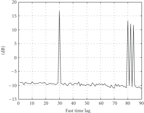
0 10 20 30 40 50 60 70 80 90
−15
−10
−5 0 5 10 15 20
(dB)
Fast time lag
(a) Scenario 1: all TSI paths have lags which are integer multiples of the range resolution, the interference power in the look direction is 10 dB and consists of four TSI arrivals corresponding to lags 30, 80, 82, and 85
0 10 20 30 40 50 60 70 80 90
−15
−10
−5 0 5 10 15 20
(dB)
Fast time lag
(b) Scenario 2: as in scenario 1, except that the noise floor has been in-creased by a factor of four and the first TSI path is now at a lag of 30.5 units
Figure4: The output of the TSI finder in the lag domain.
array broadside, (ϕ1,θ1) = (0◦, 0◦), with an interferer to
noise ratio of 10 dB (=σ2j), whereσ2n=1 is set without loss of generality. Four TSI paths are simulated with power levels β21 =1/20,β22 =1/40,β23=1/80 andβ24 =1/90. The corre-sponding TSI angles of arrival pairs are given by (ϕ1,1,θ1,1)=
(10◦,−3◦), (ϕ1,2,θ1,2)=(0◦,−20◦), (ϕ1,3,θ1,3)=(0◦,−30◦)
and, (ϕ1,4,θ1,4) = (0,◦−35◦). The corresponding fast time
lags are 30, 80, 82, and 84, respectively. The second inde-pendent interferer is 10 dB above noise and has an angle of arrival pair (ϕ2,θ2) =(20◦,−40◦). For the second
interfer-ence source we have added one multipath with parameters (ϕ2,1,θ2,1)=(30◦,−15◦),β2=1/20. In this study we will
as-sume the direction of arrival of the interferer has been iden-tified to be the array’s broadside and do not display the di-rection of arrival spectrum (a well-established capability). Figure 4(a) shows the output of the lag domain TSI finder as defined in (15). The postprocessor identifies all the TSI ar-rivals and their associated fast time lags very clearly in the simulation. The presence of the second interference source and its multipath does not visibly affect the processing gain of the TSI spectrum (spectrum is almost the same, with or without the second interference and its multipaths for the ar-ray of 16×16 elements, this is due to the high degree of free-dom available in a 256 element array). TSI spectrum is de-signed to puck up every delayed version of the look direction interferer only (by an integer multiple of the range resolu-tion, as we can scan through all possible fast time lag values). Also, the TSI spectrum excludes the look direction of the in-terferer itself. In other words, the spectrum contains only the multipaths of the look direction interferer. Further it was no-ticed that if the number of sidelobe interference sources and their multipaths increases, then the TSI spectrums which is related to the mainlobe interferer gradually looses its pro-cessing gain by increasing the noise floor. This is expected in any array processor due to its degree of freedom limitations.
This effect is really not significant until 6 or more interferes are introduced for this simulated example with 16×16 el-ements. For this simulation, we have generated 2000 range samples (≈4×2N. where 2N×2N is the size of the space time covariance matrix). Processing gain is much better than the theoretically expected values. For the smallest peak, that is, forβ24=1/90, the theoretical expectation of the process-ing gain is aroundO(4×256×(1/90)×10)≈20 dB whereas in the simulation this peak rises more than 20 dB above the average output noise floor level inFigure 4.
The simulation study has shown that the usual 3×2N(= number of samples) rule seems to be sufficient in averaging the covariance matrix in order to obtain better than the the-oretical predicted processing gain levels. The computational complexity of the TSI finder is of the order ofN3(for anN
element array) which is expected as it requires to invert the covariance matrix in (15).Figure 4(b)illustrates the results when the noise floor is increased by a factor 4 (σ2=4). The
raise can be continued until the mainlobe interferer is rea-sonably above the noise floor (at least 3 dB for this array). Due to high signal processing gain of the TSI finder, one is able to detect very weak TSI signals (β2 <1/40) of the main lobe interferer provided the direct interferer power is 3 or 4 dB above the noise level. A large number of simulation runs have confirmed that when the TSI path is not an integer mul-tiple of the range resolution, the performance degradation in the TSI spectrum is less than 1 or 2 dB at most. This was car-ried out by linearly interpolating generated TSI path data and shifting it by a fraction of the fast time lag.
40 20
0
−20
−40 −40 −20 0
20 40 0
−20
−40
−60
−80
−100
(dB)
Azim uth
Elevation
(a) 3D plot of the output of the angle finder
−30 −20 −10 0 10 20 30
−80
−70
−60
−50
−40
−30
−20
−10 0
(dB)
Azimuth (deg) (b) The azimuth cut across the peak point
−30 −20 −10 0 10 20 30
−90
−80
−70
−60
−50
−40
−30
−20
−10 0
(dB)
Elevation (deg) (c) The elevation cut across the peak point
Figure5: Output of the angle domain TSI finder where the desired lag is fixed at 30. Peak occurs atϕ=10◦,θ= −3◦.
Suppose the angle of arrival of one of the TSI paths is used to estimate the distance to the interferer by setting
1.5 2 2.5 3 3.5 4 4.5 5 5.5 6 12
14 16 18 20 22 24 26 28 30
Output
SNR
(dB)
Sample size/2N
Figure6: Estimated SNR for each iteration (data points) and mean estimated SNR (the line) at lag 30 in scenario 1, plotted against the number of samples used in the space time covariance matrix (2N×
2N) expressed as a multiple of 2N.
Δ = 0. For example ifh = 4000 meters,m = 5600,ϕ0 =
ϕ1 = 45◦, δR = 1 meter, the estimate for D is approxi-mately 4057 meters. However, ifhis changed to 0.9h(which is equivalent to havingΔ=0.1h) we haveD=3122 meters. This implies a sensitivity of around 20% due to the change of 10% in the input parameterhfor the chosen set of input values. One can always estiamte a reasonable confidence level of each estimation for the interfer distance when more than one multipath is being used. This of course depends on the ability to estimate a reasonable mean value of the parameter Δ. Other cases which we are not able to simulate or predict is the fact that the naturally scattering coefficients fluctuate. Another potential problem is the rays from the direct path and those from the TSI path may not intersect always. Hence, in practice we may be limited to making only a very crude as-sumption as the distance of the interference source.
In order to provide a wider investigation of the perfor-mance of the TSI finder as a function of the sample size used, we have included (Figure 6) a Monte Carlo simulation of sce-nario 1. Ninety simulations were run, and an estimate of the output SNR was generated at a lag of 30 (seeFigure 4(a)) as a function of the number of samples used in estimating the co-variance. InFigure 6, the number of samples used has been expressed as a multiple of the dimension of the size of the space time covariance matrix (2N×2N).
8. CONCLUDING REMARKS