VORTEX FORMATION AND DRAG ON LOW ASPECT RATIO, NORMAL FLAT PLATES
Thesis by
Matthew James Ringuette
In Partial Fulfillment of the Requirements for the Degree of
Doctor of Philosophy
California Institute of Technology Pasadena, California
2004
© 2004
Acknowledgements
First, I would like to thank Michele Milano, whose friendship, guidance, and advice on time management helped to make this work possible. Many other group members, past and present, also helped along the way. In particular, I would like to thank Dana Dabiri, Paul Krueger, and David Jeon for their assistance with DPIV, lasers, and getting the Towing Tank running again. I would also like to acknowledge Phillip Zukin, John Dabiri, Tait Pottebaum, Flavio Noca, and Derek Lisoski, for their help with various aspects of the project. Most importantly, I would like to thank my advisor,
Professor Mory Gharib. He gave me the freedom and trust to pursue my interests, encouraged creativity, provided ideas and direction when they were needed, stressed clarity and understanding, and taught me how do science that is both fascinating and relevant.
I also want to acknowledge Professor Anthony Leonard, who acted as my second advisor. His door was always open when I had a problem or idea that I wanted to go over. A discussion with Professor Leonard always resulted in understanding rooted in fundamentals, and new directions to consider.
Additionally, I would like to thank my committee, Professors Mory Gharib, Anthony Leonard, Michael Dickinson, and Joel Burdick, for their evaluation of this work and their
suggestions, which led to a more solid final product. I also want to thank Professor Hans Hornung, who served on my candidacy committee.
My wonderful family and friends, who have supported and encouraged me throughout this endeavor, also deserve mention. Particularly my wife Jen, my mother, who kept me in touch with my family and reality, and my father, for his council, spiritual guidance, and friendship. I was also fortunate to have a great friend, Joel Tse, journey west to California with me, and, thanks to the divine hand and irony of Providence, head back east at the same time I did, each to pursue his own adventures.
Abstract
Experiments were done in order to investigate the role of vortex formation in the drag force-generation of low aspect ratio, normal flat plates, with a free end condition, starting from rest. This very simplified case is a first, fundamental step toward understanding the more complicated flow of hovering flight, which relies primarily on drag for propulsion. The relative importance of the plate’s free end, or tip, with varying aspect ratio (AR) was also studied. Identifying the relationship among AR, vortex formation, and drag force can provide insight into the wing AR’s and kinematics found nature, with the eventual goal of designing man-made flapping wing micro air vehicles (MAVs).
The experiments were carried out using flat plate models in a towing tank at a moderate Reynolds number of 3000. An attached force balance measured the time-varying drag, and multiple, perpendicular sections of the flow velocity were measured quantitatively using digital particle image velocimetry (DPIV). Finally, since the flow is highly 3-D, flow visualization was done to characterize its structure and to augment the 2-D DPIV data. Two AR’s, 6 and 2, were considered, the latter in order to have a highly tip-dominated case.
responsible for the force generation in hovering flight. Vorticity fields and circulation were calculated from the DPIV data to identify any relationship between these vortices and features found in the drag force.
The effect of the plate’s tip or free end is to induce a highly 3-D, low-pressure flow that keeps the LEVs near the tip attached to the plate. Chordwise DPIV data show that the accumulation of circulation in these LEVs is restricted, as compared to the LEVs away from the tip, creating a spanwise pressure gradient within the LEVs. This pressure gradient is responsible for spanwise flow within the cores of the LEVs, directed away from the tip, which gives them a helical or tornado-like structure.
For AR = 6, the “grazing,” or nominally 2-D, lower end condition results in a minimum in the drag force at about 5 chord lengths of travel. A previous study attributed this minimum to the formation of a low-drag, recirculating LEV bubble along the span. The free end case generates instead in a drag maximum, about 46% higher, at the same distance. Chordwise and spanwise DPIV show that this maximum corresponds to the saturation of circulation within the strong LEVs at 50% span, and to the accumulation of attached vorticity near the tip, generated by the free end itself. This attached vorticity is a region of low
The flow for AR = 2 is very similar spatially to that of AR = 6, in terms of absolute distance from the plate tip. However, the AR = 2 flow evolves faster in time, implying that the effect of the tip increases with decreasing aspect ratio.
Table of Contents
Acknowledgements iii
Abstract v
List of figures xii
List of symbols xiv
1 Introduction and background 1
1.1 Introduction 1
1.2 Background 4
1.2.1 Hovering flight in nature 4
1.2.2 Flat plate starting flow and aspect ratio effects 8
1.3 Objectives and organization 14
2 Parameters 16
2.1 Introduction 16
2.2 Experimental parameters 16
2.2.1 Model geometry 16
2.2.2 Aspect ratio 17
2.2.3 Reynolds number 17
2.3 Vortex formation time 18
3 Experimental setup and methods 26
3.1 Introduction 26
3.2 Towing tank 26
3.2.1 Towing tank description 26
3.3 Flat plate models and kinematics 31
3.3.1 Flat plate model materials and dimensions 31
3.3.2 Run kinematics 33
3.4 Dye flow visualization 33
3.5 Force measurements 35
3.5.1 Force balance 35
3.5.2 Flat plate model clamp 37
3.5.3 Amplifier and data acquisition 37
3.5.4 Towing tank noise and signal conditioning 38 3.6 DPIV system 40
3.6.1 DPIV 40
3.6.2 DPIV hardware setup 40
3.6.3 DPIV processing 42
4 Results 44 4.1 Introduction 44
4.2 Force measurements 44
4.2.1 Aspect ratio 6 44
4.2.2 Aspect ratio 2 51
4.2.3 Drag force components 54
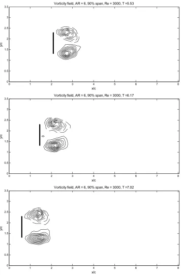
4.3 Chordwise flow sections: DPIV, circulation, and formation number 58 4.3.1 Aspect ratio 6 58
4.4.1 Introduction 103
4.4.2 Aspect ratio 6 103
4.4.3 Aspect ratio 2 117
4.5 Dye visualization and flow features explained 141
4.5.1 Introduction 141
4.5.2 Vortex line model of the startup 141
4.5.3 Global flow 146
4.5.4 Connection between corner and global flow 154 4.5.5 The decrease in LEV circulation near the tip 157
4.5.6 Mid-chord vorticity features explained 158
4.5.7 Comparison of the flow structure with previous studies 160
5 Summary and conclusions 167
5.1 Summary and conclusions 167
5.1.1 Objectives and methods 167
5.1.2 Force measurements 168
5.1.3 Chordwise flow sections: vorticity, circulation, and formation number 171 5.1.4 Spanwise and chordwise flow sections, and measured drag revisited 172 5.1.5 The structure of the flow from dye visualization 174
5.1.6 Comparison with previous work 176
5.2 Recommendations for future work 180
References 182
Appendix 186
A1.1 PMAC program for carbon fiber plate, standard velocity profile 186 A1.2 PMAC program for carbon fiber plate, ramp velocity profile 187 A1.3 PMAC program for glass plate used for DPIV, standard velocity profile 188 A1.4 PMAC program for glass plate used for flow vis., standard velocity profile 189
List of figures
Figure 2.1 Circulation at AR = 6, 50% span, with vorticity field insets 23 Figure 3.1 Towing tank and hardware for DPIV and flow visualization 27
Figure 3.2 Schematic of force balance 36
Figure 3.3 CD from amplifier output vs. averaged & digitally filtered CD 39 Figure 3.4 Circulation calculated from filtered and unfiltered vorticity data 43 Figure 4.2.1 Measured CD vs. formation time, AR = 6 45 Figure 4.2.2 Measured CD vs. formation time, AR = 2 and 6 52 Figure 4.2.3 Measured CD vs. real time, AR = 6, acceleration over 2.5c 56
Figure 4.3.1 Circulation vs. formation time, AR= 6 59
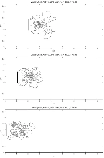
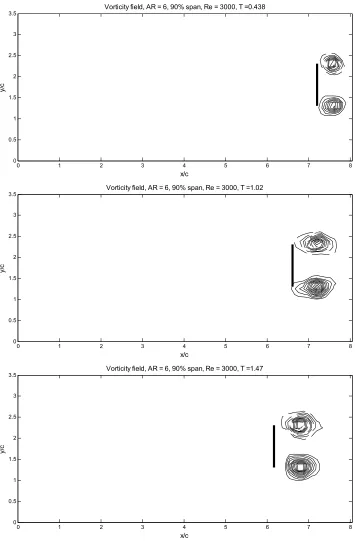
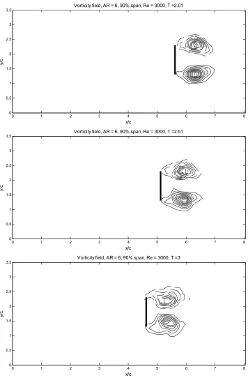
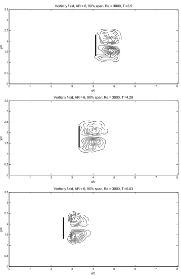
Figure 4.3.2 Circulation at AR = 6, 50% span, with vorticity field insets 62 Figure 4.3.3 Circulation at AR = 6, 75% span, with vorticity field insets 64 Figure 4.3.4 Circulation at AR = 6, 90% span, with vorticity field insets 66
Figure 4.3.8 Circulation vs. formation time, AR= 2 68
Figure 4.3.9 Circulation at AR = 2, 50% span, with vorticity field insets 70 Figure 4.3.10 Circulation at AR = 2, 75% span, with vorticity field insets 72 Figure 4.3.11 Circulation at AR = 2, 90% span, with vorticity field insets 74 Figure 4.3.5 Evolution of the vorticity field for AR = 6, 50% span 76 Figure 4.3.6 Evolution of the vorticity field for AR = 6, 75% span 80 Figure 4.3.7 Evolution of the vorticity field for AR = 6, 90% span 84 Figure 4.3.12 Evolution of the vorticity field for AR = 2, 50% span 88 Figure 4.3.13 Evolution of the vorticity field for AR = 2, 75% span 93 Figure 4.3.14 Evolution of the vorticity field for AR = 2, 90% span 98 Figure 4.4.1 Circulation of the AR = 6 tip vortex seen in the mid-chord plane 105 Figure 4.4.2 Measured CD vs. T for AR = 6 (part 1), including tiled vorticity insets to
show the flow at significant formation times 113
Figure 4.4.3 Measured CD vs. T for AR = 6 (part 2), including tiled vorticity insets to
show the flow at significant formation times 114
Figure 4.4.4 Measured CD vs. T for AR = 2 (part 1), including tiled vorticity insets to
show the flow at significant formation times 115
Figure 4.4.5 Measured CD vs. T for AR = 2 (part 2), including tiled vorticity insets to
show the flow at significant formation times 116
Figure 4.4.8d Tiled vorticity fields for AR = 2, T= 2.8 135 Figure 4.4.8e Tiled vorticity fields for AR = 2, T= 3.75 136 Figure 4.4.8f Tiled vorticity fields for AR = 2, T= 4.39 137 Figure 4.4.8g Tiled vorticity fields for AR = 2, T= 5.73 138 Figure 4.4.8h Tiled vorticity fields for AR = 2, T= 6.77 139 Figure 4.4.8i Tiled vorticity fields for AR = 2, T= 7.51 140 Figure 4.5.1 Vortex line model of the flow near the tip at the startup 142 Figure 4.5.2 Comparison of dye blob visualization with vortex line model 144 Figure 4.5.3 3-D dye visualization. Re = 2000, AR= 6 147 Figure 4.5.4 3-D dye blob visualization, isometric view of leeward face of plate. Re =
2000, AR= 6 149
Figure 4.5.5 Tiled vorticity plots, for AR = 6, from section 4.4 illustrating the connection between vorticity in the leading edge plane and LEV core locations in the
chordwise planes 151
Figure 4.5.6 Bifurcation of tip vortex into helical corner vortex and a smaller, outboard
tip vortex near the leading edge 153
Figure 4.5.7 Dye blob vis., AR = 6, Re = 3000, reconciling corner vortices & the main
LEV 156
Figure 4.5.8 Mid-chord plane dye visualization, Re = 3000. Dye from the plate corners is convected into the mid-chord plane above the tip vortex 159
List of symbols Roman symbols
A area over which circulation is computed AR aspect ratio
b plate span
c plate chord length CD drag coefficient D drag
h plate thickness Re Reynolds number t time
S plate area
T formation time
T* non-dimensional time, T* = tU/c U plate velocity
Ufinal final, constant plate velocity U mean of plate velocity, U Greek symbols
α angle of attack (degrees) Γ circulation
ν kinematic viscosity
ρ density (typically of water)
ω vorticity component normal to the plane under consideration Abbreviations
DPIV digital particle image velocimetry LEV leading edge vortex
1 Introduction and background 1.1 Introduction
In recent years there has been a push to understand biological flight. Observation of a honeybee in a flower garden or a fly in the house reveals the reasons why. Flying animals are capable of extraordinary acrobatic maneuvers and operating in confined spaces. They also offer lessons in control system and actuator design. Biological inspiration coupled with a clear understanding of the underlying physics could lead to man-made devices with similar or superior capabilities. Micro air vehicles (MAVs), as such creations are called, would have military and civilian applications, such as reconnaissance and search and rescue.
A feature common to all creatures able to hover, namely, most flying insects and hummingbirds, is the low aspect ratio of their wings. Aspect ratio (AR) will be defined throughout this work as b2 S, where b is the span of a single wing, instead of the
conventional definition, which is the distance between both wing tips; S is the single-wing planform (top-view) area. Flying insects have AR’s between about 2.75 and almost 6, (Ellington, 1984; Dickinson, 1999), while hummingbirds have AR’s of around 4 (Dhawan, 1988); a soaring animal, such as the albatross, has an AR of about 9 (Dhawan, 1988). A finite AR wing, versus one of infinite span, experiences aerodynamic effects due to the tip, which increase relatively as the AR decreases. Therefore, for low AR wings, the influence of the tip is very significant.
The flow over a wing undergoing hovering kinematics is necessarily unsteady: during one half-stroke, the wing accelerates and rotates, all while traveling a distance of only about 3 to 5 chord lengths (Weis-Fogh, 1973; Wang et al., 2004). Separation occurs at the edges of the wing, due to the high angles of attack and the sufficiently high velocities. This results in the formation of wake vortices at the leading and trailing edges, as well as at the tip
Upon performing flow visualization using a robotic model of a flapping hawkmoth, Ellington et al. (1996) observed significant spanwise flow (from wing root to tip) within the LEV core, which they attributed to a corresponding spanwise pressure gradient due to the higher velocities of the wing tip. They hypothesized that this spanwise flow drains some of the vorticity of the LEV outboard to the wing tip. This, they postulated, retards the vorticity accumulation in the LEV, as compared to the 2-D case (Dickinson & Götz, 1993), so that more time is required for the vortex to build up enough circulation to shed. Birch and Dickinson (2001), using digital particle velocimetry (DPIV) to measure the velocity field around a flapping robotic model of a fruitfly, found only a very small spanwise velocity in the LEV. Additionally, they observed a large tip vortex (TV) attached to the wing, which induced spanwise flow behind the LEV, near the wing’s trailing edge, as well as a strong downward flow around the wing; the flow from the previous wing stroke also contributed to this downward flow. Birch and Dickinson proposed an alternative hypothesis that of
Ellington et al., which is that this induced downward flow, or downwash, significantly lowers the effective angle of attack of the wing, compared to a purely 2-D case, thus retarding the growth of the LEV and increasing its time to shed. Although Ellington et al. also reported a large TV, after the middle of the downstroke, they only commented that the outboard portion of the LEV breaks down and “feeds” into it. Therefore, there is disagreement over the mechanism that keeps the LEV attached to a 3-D, hovering wing longer than its 2-D
counterpart. Moreover, the importance of the TV, and its effect on the LEV, is in dispute. In order to investigate the roles of the LEV and the TV in the force generation during something as complicated as hovering flight, the philosophy that it is better to start by
the wing is modeled as a low AR flat plate of rectangular planform. The α is 90°, so that drag is the primary force that the plate experiences. Since each half-stroke has essentially mirror-image force generation, only one half-stroke will be modeled. Consequently, the problem reduces to an investigation of the vortex formation and force generation of a low AR flat plate accelerating from rest, oriented normal to its direction of travel. A brief history of previous work related to this problem must therefore include studies from the fields of biology and fluid mechanics. The literature pertaining directly to biological hovering will be discussed first, followed by a review of past studies on flat plate starting flow and AR effects.
1.2 Background
1.2.1 Hovering flight in nature
One of the first major investigations of hovering animals was done by Weis-Fogh in 1973. It contains a very thorough study of the many aspects of hovering flight, including aerodynamics, power, efficiency, wing kinematics, and some hypothesized unsteady lift-generation mechanisms such as the “clap” and “fling.” His observations on hovering kinematics are especially applicable to the present work. Weis-Fogh found that most hovering animals exhibit similar kinematic behavior, which he thus called “normal hovering.” He defined normal hovering kinematics as the animal flapping its wings
to explain the aerodynamic performance of most hovering animals, which severely limits the applicability of his results.
In 1984 Ellington published a 180-page, 6-part paper on the aerodynamics of insect hovering flight. It provides a detailed analysis of wing geometry, improved kinematics data, a discussion on aerodynamic mechanisms, and information on lift and power requirements. Ellington confirmed Weis-Fogh’s observation that most hovering animals flap their wings in a horizontal stroke plane, but disagreed with Weis-Fogh’s use of the quasi-steady flow
assumption. More importantly, he examined the idea that vorticity generated by separation at the edges of the wing could be a lifting mechanism for hovering flight. Based on
experiments by Maxworthy (1979), he speculated that the LEV may be the primary lift-generating vortex, and that the induced spanwise flow (from root to tip) due to the TV may keep the LEV from shedding throughout each half-stroke. Technological advances during the 1990’s allowed for more advanced experiments to test these hypotheses.
In the study by Ellington et al. (1996), discussed in section 1.1, 3-D flow visualization was also performed on an actual hawkmoth flapping in a wind tunnel. These results, coupled with the flow visualization done on their robotic flapping model of the hawkmoth, provided new insight into hovering flight. As reported above, they observed a strong LEV during the downstroke, and spanwise flow within the LEV core from the wing root to the tip. They also found that the LEV had a helical structure similar to that of a delta wing, and they
mentioned above, increases the time needed for the vortex to build up enough circulation to shed. During the latter half of the downstroke, the LEV was seen to merge with a large TV, but whether the TV itself was partly responsible for the spanwise flow in the LEV was not discussed.
second LEV, both of which are finally shed at the end of the half-stroke. Again, whether or not the tip vortex itself is responsible for any force generation or the spanwise flow in the first LEV is not discussed.
As described in section 1.1, experiments done by Birch and Dickinson (2001) using a robotic model of a flapping fruitfly showed only a very small spanwise velocity component within the LEV core. They also observed a large TV, which, along with wake vorticity shed from the previous stroke, induced a strong downward flow about the wing. Further
experiments were done to suppress any spanwise flow in the LEV (which had little effect), and to hinder the development of the TV by placing a wall at the wing tip, geometrically matched to the tip’s trajectory. The latter experiment increased the strength of the LEV by 14%, and the overall force on the wing by 8%, although, interestingly, the LEV still did not shed; for the fruitfly, apparently, LEV strength, not shedding, is the force-limiter. These results led to the hypothesis that the prolonged attachment of the LEV is instead due to the aforementioned downwash from the TV and the previous stroke’s wake. This downward flow, they postulated, lowers the effective angle of attack of the wing, thus decreasing the strength of the LEV and increasing its time to shed. Therefore, there is some controversy as to the role of the tip vortex in hovering flight. However, Birch and Dickinson noted that hawkmoths fly at Reynolds numbers of around 2000, while for fruitflies the Reynolds number is between 100 and 250. They suggested that the pressure gradient along a fruitfly wing may simply be too small to generate significant spanwise flow.
To the best of this author’s knowledge, no study has yet explored the force generation due to the TV and its effect on the LEV, at Reynolds numbers on the order of 1000.
100) done by Ramamurti and Sandburgh (2002) show that, for the case of symmetric (up- and downstroke) flapping kinematics, almost half of the total thrust is generated by the outboard 25% of the wing. Given this result and that the TV has been implicated in prolonging the attachment of the LEV, a further study of their interaction, and how it is affected by aspect ratio, is warranted.
1.2.2 Flat plate starting flow and aspect ratio effects
There is a great wealth of literature on bluff body flows. Much of it is concerned with circular cylinders, due to their many engineering applications. Of the studies on flat plates normal to the direction of travel, there are few that deal with the unsteady flow at the startup of motion; and there are virtually none that investigate low aspect ratio flat plates having a free end condition. Most studies present results on long time behavior, such as Strouhal shedding frequency, and mean and fluctuating force coefficients (see Lisoski (1993) for a thorough review). Some of the more well-known of these works are by Fage and Johansen (1927) and Roshko (1954; 1955).
Nominally 2-D flat plate starting flow was investigated experimentally by Sarpkaya and Kline (1982), Lian and Huang (1989), Dickinson & Götz (1992), and Dennis et al. (1993); experiments and computations were conducted by Chua et al. (1990) and Lisoski (1993); and Koumoutsakos and Shiels (1996) presented viscous computational simulations. Highlights from these investigations will now be summarized.
U is the free stream velocity, t is time, and c is the plate chord length. They found a peak drag coefficient (CD) of about 3 at T* = 1, followed by a decrease to CD = 2.4 until T* of around 5, leveling off to an average CD of 2.2 after T* = 6 (measured out to T* = 13). The large initial CD was attributed to the symmetric growth of the starting vortices generated by the plate’s 2 edges, and it was noted that shedding did not cause noticeable fluctuations in the CD.
The experiments done by Chua et al. (1990) investigated the unsteady forces on a normal flat plate accelerating from rest in a towing tank to a constant velocity. The plate was accelerated until T* = 2, then driven at a constant Re of 5000, with a total travel of 60 chord lengths. Initially, they measured a peak in the CD of 4.5 at T* = 2, which then dropped off to a minimum of 1.7 at T* = 8, and finally rose to an average of 1.9 after T* = 12. Although the CD magnitudes are somewhat similar to Sarpkaya and Kline’s, no drag minimum was
observed in the previous study. This difference may be due to the difference in velocity profiles, or possibly Reynolds number, although Chua et al. obtained the same result for Re = 5000 and 10000. Using flow visualization, Chua et al. attributed this significant drag
minimum, or “bucket,” to the existence of a “symmetric vortex bubble region” behind the plate, which broke up at T* = 10. Force measurements and visualization showed no vortex shedding between T* = 12 and 30 to 40, after which shedding began and caused fluctuations in the CD. The computations by Chua et al. did not agree well with their experiments for the starting flow case, probably due to unavoidable three-dimensionality in the experiments.
for small insects such as fruitflies. A wall at each end of the wing ensured that the flow was primarily 2-D. They found that, for this essentially 2-D case, the LEV shed into the wake after about 2 chord lengths of travel. This distance, as discussed before, is shorter than the typical insect wing stroke amplitude of 3 to 5 chord lengths.
For their largest angle of attack, α = 90°, with a total travel of 7 chord lengths at a Re of 192, their measured CD agrees quite well with the results of Sarpkaya and Kline (1982), albeit with a higher initial peak CD. The drag “bucket” measured by Chua et al. (1990) at T* = 8 was not observed by Dickinson and Götz. This might be because their experiments did not go beyond 7 chord lengths of travel, or that their Re was so low that the recirculating wake bubble persisted throughout the entire run, and would have done so beyond 7c.
In 1996, Koumoutsakos and Shiels used vortex methods to compute the 2-D viscous flow around impulsively started and uniformly accelerated flat plates oriented normal to their direction of travel. The impulsively started case, computed at Reynolds numbers between 20 and 1000, agreed well with the flat plate flow visualization study of Dennis et al. (1993) for early times, when the experimental flows were still essentially 2-D. The longer-time CD’s (between 0.8 and 1.2 for Re = 20 to 40, T* > 10) for both studies also agreed well; the computed CD was infinity at time t = 0, and therefore not amenable to comparison. For the uniformly accelerated plate, Koumoutsakos and Shiels were the first to confirm
computationally the existence of an instability along the shear layers emanating from the plate’s edges, manifested as “centers of vorticity.” This instability was observed
angles. Pullin and Perry speculated that the instability was triggered by vibrations, although very small, in their experimental apparatus, while Lian and Huang concluded that this instability is inherent to the flow. Koumoutsakos and Shiels also determined that the instability is in fact a feature of the flow. They showed that it is caused by the oscillatory behavior of the interaction of primary and secondary vorticity at the plate edges, which triggers Kelvin-Helmholtz-like instabilities in the shear layer.
Lisoski’s Ph.D. thesis (1993) at the California Institute of Technology continued the work he contributed to Chua et al. (1990). He investigated experimentally and
computationally the effect of “differing amounts of large-scale and small-scale three dimensionality” on the time-varying flow about a normal flat plate at Reynolds numbers between 1000 and 6000. Large-scale three-dimensional effects were studied using flat plate models with varying end conditions and aspect ratio, with the objective of determining how best to suppress these effects. The starting and intermediate-time flow, with the plate traveling a total of between 60 and 100 chord lengths, was studied in the same towing tank used in the present experiments. Longer-time flows were investigated in a water tunnel, which allowed runs equaling thousands of chord lengths. Force measurements and flow visualization were used to compare the experiments with one another, and with the results from a 2-D vortex element code.
large-scale three-dimensionality was effectively suppressed: the results from AR = 6 to 17 were very similar. However, with an AR = 10 and the free end of the model significantly far away from the tank bottom, the drag “bucket” measured for his most nominally 2-D case (AR = 17, grazing), and reported in Chua et al. (1990), was not observed. In addition, Lisoski noted that this free end condition “... effectively suppressed organized vortex shedding [which occurs beyond T* = 30 to 40] at both AR = 10 and AR = 17.”
Lisoski’s water tunnel experiments revealed that, for AR = 6 with an end plate
mounted on the model, vortex shedding was intermittent, being absent for hundreds of chord lengths of travel at a time. This was evident in the time-varying drag and lift measurements, which showed little variation during periods of no shedding. Periodic vortex shedding was consistently observed, however, for AR’s greater than 10, and no shedding was observed for AR = 4. Lisoski found that, when vortex shedding did occur for AR’s ≤ 6, the flow lacked spanwise correlation. This decreased the drag by almost 40%, and suppressed the usual force oscillations at the Strouhal frequency. Finally, Lisoski concluded that the flow for AR ≤ 6 plates, with their free end far away from the bottom wall, is significantly three-dimensional, but that higher AR plates with the same end condition probably have some portion along the span that exhibits primarily 2-D flow.
cylinder with its end free and far away from the tank floor was studied, and they showed that vortex shedding near the end of the cylinder is suppressed; it only occurs 3 to 4 diameters from the end. Additionally, they observed that the oncoming flow near the free end is deflected upward, and that dye deposited on the end itself is “... drawn upwards into the wake, close behind the cylinder.” This causes the wake vortices to bend toward the tip, which is seen in a side-view of the flow. After this “bowing” is observed, the vortex
interactions near the tip become complicated. Slaouti and Gerrard wrote that “[a] contraction of the wake is thus gradually obtained as the lowest sections of the vortices disappear with downstream distance through cancellation of their vorticity due to mixing.”
In 1992, Champion and Coutanceau presented a short paper at the IUTAM
Symposium on Bluff-Body Wakes, Dynamics and Instabilities entitled “Development of the Near Wake Structure on a Cantilevered Circular Cylinder with a Free-End.” They
characterized this highly three-dimensional flow qualitatively using 3-D dye flow visualization, as well as time-exposed 2-D particle visualization for multiple chordwise cross-sections and a spanwise section bisecting the wake. A similar approach was used in conjunction with DPIV for the present study, so that flow cross sections could be captured quantitatively. Champion and Coutanceau tested cylinders with AR’s between 2 and 5 in a vertical water tank, at Re = 1000. One end of the cylinder was of course free, and a flat plate was mounted at the other end. Their multiple visualizations allowed for a temporal and spatial picture of the time-evolving near-wake. For the case of AR = 5, at T* = 2
vortices show a “quasi-2-D development.” However, the flow near the free end remains very near to the cylinder and is highly 3-D, due to spanwise flow directed toward the fixed end. By T* = 3.5, the vortex lines in the spanwise region 1 ≤ Z/D ≤ 3.5 have bowed-out away from the cylinder, and are also asymmetric. However, the vortices near the free end remain
closely attached to it, and no vortex shedding is seen. This same bending-in of the vortex lines toward the free end was observed by Slaouti and Gerrard (1981). Near the end plate, the vortices stay attached to the cylinder but become very 3-D and irregular, versus the clean free surface end condition used by Slaouti and Gerrard, which promotes 2-D flow.
The 3-D dye visualization revealed that the vortices generated near the free and fixed end have a helical structure. They propagate along the span in opposite directions, heading towards Z/D = 2, where they collide. This meeting of helical vortices propagating in opposite directions was also observed Liu et al. (1998). During the latter-half of the hawkmoth’s downstroke, the helical LEV over the inboard 75% of the wing (which has a spanwise velocity component directed toward the tip) connects with the outboard helical LEV (that has a velocity directed away from the tip), and the spanwise flow at that location is reduced to zero.
Lastly, Champion and Coutanceau commented on the effects of decreasing the cylinder aspect ratio. They noted that the length of the recirculating bubble increases, as does its stretching speed. Also, the spanwise location where the helical vortices traveling in opposite directions collide was seen to be a linear function of AR.
1.3 Objectives and organization
begin to understand the fundamental physics of hovering flight. In addition, the effect of varying the AR, which changes the relative influence of the plate’s tip or free end, was explored to gain insight into AR selection in nature and for MAV design.
These goals were achieved through drag force measurements, quantitative
measurements of multiple sections of the flow velocity, 2-D and 3-D flow visualization, and the formation time concept. The formation time is a non-dimensionalized timescale that can be used to relate the time it takes for a vortex to reach its final strength before pinch-off with the kinematics that generated it. Using this timescale, vortex saturation can be compared with other kinematics-dependent phenomena, such as peaks in the drag force. Measuring the drag on different AR plates, as well as varying their end conditions, establishes the relative importance of the tip effect for force generation. Using digital particle image velocimetry (DPIV), multiple chordwise and spanwise (2-D) sections of the flow velocity were captured quantitatively, in order to obtain vorticity and circulation data for the LEVs and the TV. This data allowed vortex formation, strength, and interaction to be related, through the formation time, to features in the measured force. Finally, flow visualization was used to choose the appropriate experimental parameters, obtain a picture of the full 3-D flow, and explain the DPIV results.
A more detailed discussion on the formation time concept and the experimental parameters chosen for this work is given in Chapter 2. Chapter 3 describes the experimental setup and techniques, and the results are reported in Chapter 4. Conclusions and
2 Parameters 2.1 Introduction
The parameters and concepts relevant to this work are presented in this chapter. First, the experimental parameter selection is explained. Following this is a discussion on the vortex formation time theory, which was first used to characterize vortex ring formation, and has also been applied to circular cylinder starting flows. Formation time relates the growth and final strength of a vortex to the kinematics of the system that generated it, and is thus very useful for understanding vortex-based propulsion. Therefore, formation times for the plate’s 2 LEVs and its TV are defined, and their physical meaning is discussed.
2.2 Experimental parameters
A flat plate of rectangular planform was chosen as the experimental model because it is one of the simplest representations of a thin flapping wing appendage. Additionally, having three distinct edges (the fourth is outside the working fluid) allows for predictable vortex generation: 2 vortices (the LEVs) will form at the long edges, while a tip vortex will roll up over the short edge; Chapter 4 will show that vortices also form at the plate’s corners. Although insect and especially bird wings deform, the models tested did not include this variable. Dickinson et al. (1999) found that exchanging the rigid wings for flexible ones on their robotic fruitfly did not affect the forces appreciably, but this is probably due to their low operating Reynolds numbers. An angle of attack of 90 degrees was selected in order to ensure that the force generation would be primarily drag-based, which is consistent with hovering flight.
2.2.2 Aspect ratio
The range of aspect ratios tested was based on biological data and previous work in fluid mechanics. In Chapter 1, it was stated that insect single-wing AR’s range from 2.75 to 6, while hummingbird AR’s are around 4. Also, Lisoski (1993) found significant 3-D effects for flat plates when the AR was reduced to 6, while Champion and Coutanceau (1992) observed highly 3-D flow for cantilevered cylinders with AR’s between 2 and 5. This investigation, therefore, considered two AR’s: 6, as the prototypical case, and 2, in order to have a TV dominated flow.
2.2.3 Reynolds number
performed their cylinder experiments at Re = 1000. In order to compare the present work with those studies just mentioned, and still be within the insect flight regime, a Re on the order of 1000 was chosen. Reynolds number for the current flat plate study is defined as
ν
final cU Re=
Where c is the plate chord length, ν is the kinematic viscosity of water, and Ufinal is the final, constant velocity of the plate after it accelerates from rest (see Chapter 3). Dye flow
visualization in chordwise planes at 50, 75, and 90% span (measured from the plate root) was performed for AR = 6 at Re’s of 1000, 2000, 3000, 5000, and 10000, to determine an
appropriate Re more precisely. For Re = 1000, the symmetry of the recirculating bubble behind the plate was random: most runs exhibited wake symmetry, but some runs, after about 5 chord lengths of travel, did not, probably depending on the level of background noise in the water tank.
A more repeatable flow, obtained by increasing the Re, was desirable, but the size of the shear layer instability described in Koumoutsakos and Shiels (1996) was found to scale with Re. A compromise was reached at a Reynolds number of 3000, which provided consistent results along with the least amount of contamination from the instability. The investigation was performed at only one Re, since 2-D and 3-D flow visualization showed that the flow was similar for Re between 2000 and 5000; this was true even for the Re = 10,000 case, although the shear layer instability was very large. Finally, the signal-to-noise ratio for the drag force measurements was much better at Re = 3000 versus 1000.
2.3 Vortex formation time
vortex ring formation over long timescales. A vortex ring, which is a vortex with it ends connected together, is a clean, well-studied flow, with a simple generation mechanism. Gharib et al. produced vortex rings in a water tank using a piston to push a column (or slug) of water of length L through a cylindrical nozzle of diameter D (equal to the piston diameter). The vorticity fed into a forming vortex ring is provided by the separated shear layer at the nozzle exit, which is driven by the moving piston. Stopping the piston after a certain
distance prohibits the shear layer vorticity flux, so that the final circulation of the vortex ring is approximately equal to that generated at the nozzle exit; this is true for small
D L
’s. The
question that Gharib et al. asked is the following: for large D L
’s, given a fixed mean piston
velocity, is there a limiting process that keeps the circulation of the vortex ring from growing indefinitely, despite the vorticity flux emanating from the shear layer? They found such a process by using digital particle image velocimetry (DPIV) to capture the formation, growth, and subsequent pinch-off of vortex rings generated by various piston kinematics.
In order to compare runs with different piston velocity programs and nozzle diameters, time was non-dimensionalized into what Gharib et al. (1998) referred to as
“formation time” (T) using the running average of the piston speed U and the nozzle diameter as follows:
( )
t dt DL U t D t D U t T t = = =∫
0 ' ' 1As the formula shows, formation time for this case is also equal to the stroke ratio, D L
, which
is the number of diameters the piston traveled. For small
max ⎟ ⎠ ⎞ ⎜ ⎝ ⎛ D L
compact and clean, consistent with previous studies. However, for T greater than about 4, the circulation of the vortex rings did not increase indefinitely. Instead, it saturated, and the remaining circulation generated by the shear layer at the nozzle trailed the vortex rings in a
jet-like structure. Regardless of the
max ⎟ ⎠ ⎞ ⎜ ⎝ ⎛ D L
, Gharib et al. found that the maximum
circulation of the vortex rings was acquired around T = 4, which they called the “formation number.” Jeon (2000) studied the vortex formation of essentially 2-D cylinder starting flow, and also found vortex saturation at about T = 4 for many cases. This showed that the
formation time concept can be applied to bluff bodies, and suggested that the magnitude of the formation number might be similar for different vortex generators.
The formation number is the non-dimensional time at which a vortex achieves its maximum circulation before pinch-off. Pinch-off occurs when a vortex is no longer being fed by the shear layer that generated it, and the two become distinct entities in terms of vorticity. This does not necessarily happen exactly at the formation number (it typically happens sometime afterward), but pinch-off cannot occur before the vortex acquirers its maximum circulation. The experiments by Gharib et al. (1998) showed that the pinch-off process for a vortex ring starts at around T = 4, but it is not clearly complete until T is about 7 or 8. This formation and pinch-off process will be described for low AR flat plates in this section and later chapters.
The low AR plates considered in the present work were oriented vertically in a water tank, piercing the free surface so that three edges, the two leading or side edges and the tip edge at the bottom, were underwater (see Chapter 3). As discussed above, vortices are generated at the two leading edges and at the tip of the plate as it accelerates from rest. The two LEVs rotate primarily in the horizontal plane, while the TV rotates primarily in the vertical plane. Using DPIV to obtain velocity and vorticity fields in horizontal and vertical sections (akin to the flow visualization study done by Champion and Coutanceau (1992)), formation numbers can be defined for the vortices that are visible in each section. The variation of the LEVs along the span of the plate and in time was captured using DPIV data taken at horizontal (chordwise) sections at 50, 75, and 90% spanwise locations (measured from the top). Visualization in 2-D and 3-D for AR = 6 revealed a complicated flow above 40% span after the initially 2-D vortex generation phase, which was also observed by Champion and Coutanceau. Although their root end condition was an endplate, while the upper-end condition for the present study was a clean free surface, something about the low ARs considered seems to cause significant 3-D flow at both ends of the body. Since the present work is focused on phenomena near the plate tip, only the flow away from the upper end was considered. The TV was investigated by taking DPIV data in two vertical
(spanwise) sections: one at mid-chord, parallel to the direction of travel and in the symmetry plane of the LEV wake, and one at one of the leading edges, also parallel to the plate
velocity, and within the rotating flow of the LEV there.
Formation time for the present work is defined as follows:
where c, again, is the plate chord length, and U is the running mean of the plate velocity. Since the plate is a bluff body, it is appropriate to use its chord, or frontal projected length, as the normalizing length scale. The formation time T is approximately equal to the number of chord lengths the plate has traveled, and it is very useful for comparing runs with different kinematics and chord lengths. The formation number is the formation time at which a vortex generated by one of the plate edges acquires its maximum circulation. It is found using circulation data obtained from DPIV measurements, which will now be discussed.
The case of AR = 6, Re = 3000, and DPIV data taken in a horizontal (chordwise) plane at 50% span will be used as an example of computing the formation number. The DPIV measurements provide the time-varying velocity field in an area surrounding the plate. From the velocity data, quantities such as vorticity can be calculated. At this Reynolds number and spanwise location, the starting flow is symmetric about a line at mid-chord parallel to the direction of travel. Therefore, when flow quantities at one edge, such as the circulation, are desired, the quantities at each edge can be averaged. In order to obtain the formation number, the total circulation generated at the edge as well as that within the LEV are computed from the DPIV vorticity data using Stokes’ theorem in 2-D:
∫
= ΓA
dA
ω
where ω is the vorticity, and A is the area enclosing it. A curve of total and LEV circulation versus formation time can then be constructed.
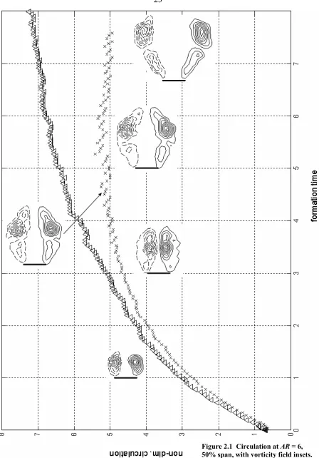
Figure 2.1 gives both the total and LEV circulation at 50% span, with insets showing the vorticity field at significant formation times. The LEV circulation was computed
manually, especially before pinch-off, is somewhat arbitrary. The total circulation was also computed using Matlab, and it is the average of the circulation generated at each edge. Initially, the total and LEV circulation are equal (see Figure 2.1). However, with time they begin to diverge, and at T equal to the formation number (in this case about 4.5), the LEVs saturate and can no longer accept vorticity from the separated shear layer that formed them. From this time on, the LEV circulation measurements are essentially constant, within the experimental error. The formation number is therefore the formation time at which the LEV circulation data become constant. After the formation number, the shear layer and the LEV then start to become separate entities (see the vorticity field inset at T = 5 in Figure 2.1). Finally, at pinch-off (T = 6.67 in Figure 2.1), the two are entirely distinct, which shows up on a vorticity contour plot as a disconnection of their contours, with a minimum of vorticity between the two. For the cases where no pinch-off exists (which occurs near the tip), formation numbers can still be computed if the circulation of the vortices saturates, despite their continued attachment to the plate.
3 Experimental setup and methods 3.1 Introduction
This chapter presents the details of the experimental setup and methods. First, the towing tank facility, where all the experiments were done, will be described. Next, the specifications of the flat plate models and kinematics are given, followed by a brief
discussion on the dye flow visualization. After that, the force balance and data acquisition system are described. Lastly, the details of the DPIV system and post-processing are given. 3.2 Towing tank
Towing tanks, as opposed to wind and water tunnels, are very useful for studying unsteady starting flows, due to their capability of accurately “towing” models at pre-programmed unsteady velocity profiles. The GALCIT towing tank was used for all the experiments done for this thesis, as its size and the velocity range of its drive system were appropriate.
3.2.1 Towing tank description
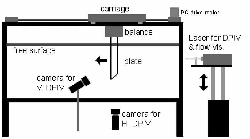
Originally designed for flow visualization (see Williamson, 1988), the tank has four uninterrupted glass side-walls, and a glass bottom covered only across its midpoint by a cross-bar support; the top is open to the air. The interior dimensions of the tank are 450 cm in length and 96 cm in width, with a depth of 78 cm. It is raised up above the ground on six legs, which can be adjusted to level it, providing space to perform visualization and acquire DPIV data from below. Figure 3.1 shows a side-view sketch of the towing tank, along with the laser and CCD camera configurations for DPIV and flow visualization.
the force balance and flat plate models are attached. The carriage is moved using a 2-pulley and cable drive system located along one of the side rails. The pulley at one end of the tank is driven by a DC servomotor combined with a gearbox, while the pulley at the opposite end is free. A smaller version of this drive system is located on the carriage itself, but oriented perpendicularly to the larger one. The force balance and model combination are actually attached to the smaller carriage of this secondary system. Thus, models can be moved in two dimensions, but only the main drive system was needed for the present work.
The DC servomotor is a PMI model OP-01206-026 (type U12M4HT/GH/M23) with an attached gearbox having a 20:1 input-to-output ratio. The motor is driven by a PMI model 00-88029-006 multi-axis switching servo amplifier (type CX-75-10-30), which obtains tachometer feedback from the motor in order to close the velocity loop for motor control. The position loop consists of an encoder and a motion controller, described next.
A PMI optical encoder with a resolution of 1024 counts per revolution is attached to the drive shaft of the DC servomotor, in order to provide position feedback to the motion controller. The gearing of the servomotor is such that there are about 1427 counts per cm of carriage travel, providing more than enough position control accuracy for this study.
Position information from the encoder is fed into a Delta-Tau Mini-PMAC (programmable multi-axis controller), which is mounted in a PC as a standard card, and thus allows the motor to be controlled by the PC. The position control loop is closed by the command signal that is sent from the Mini-PMAC to the amplifier, which in turn drives the motor in the desired manner.
Software provided by Delta-Tau allows the controller gains to be tuned, the encoder output to be calibrated, and pre-programmed motion profiles to be sent to the motor. The Mini-PMAC uses a proportional-integral-derivative (PID) control scheme to minimize the following error between the commanded an actual position of the motor. Velocity and acceleration feed-forward gains are adjusted by the user via the software, utilizing the position information from the encoder, to optimize motor performance. Once the controller is tuned, motion programs that prescribe velocity or position as a function of time can be written and used to command the motor. The software allows for an almost unlimited variety of motion trajectories, restricted only by the mechanical properties of the system, and thus affords more than adequate control of the towing tank carriage.
3.2.2 Towing tank procedures
The working fluid in the towing tank was water, and the plate upper-end condition was a clean free surface, for the reasons given in Chapter 1. Before a series of data sets was taken the free surface was cleaned, and it stayed that way for many hours. Due to the air filtration system in the laboratory, and the height of the tank above the floor, dust
contamination on the free surface was minimal. Slaouti and Gerrard (1981) noted that minor contamination of the free surface did not significantly affect vortex impingement there. To clean the free surface, a fan at one end of the tank was used to blow any debris toward the opposite end of the tank. A tube connected to a shop vac, and hovering just above the free surface, was then used to suction away the debris there. This left a clean surface that was evident by its appearance, as well as wave generation and prolonged wave action at the slightest disturbance. Some of the 10 micron particles used to seed the flow during DPIV measurements inevitably floated to the surface due to a slight density difference between them and the water, but they did not appreciably affect the behavior of the free surface. If, however, the amount of particles on the surface became large, the surface was cleaned again as a precaution.
was judged to be significantly settled when the force balance was no longer able to distinguish the ambient flow from its at-rest noise level. This typically took about half an hour. The DPIV measurements were a bit more sensitive, since the flow velocity itself is being measured, and wait-times between runs ranged from half an hour to an hour. For the DPIV experiments, the initial tank stirring coincided with seeding the water with the tracer particles. If any subsequent seeding in the middle of a series of data sets was needed, the stirring was repeated, and the flow was allowed to settle for an hour to an hour and a half.
When the GALCIT towing tank was chosen for the present work, its carriage was outfitted with wheels to roll it along the rails. Although the wheels provided very low
friction for the servomotor to overcome, and they did not require additional measures such as greasing the rails, the vibrations they transmitted to the carriage due to imperfections in the rails and their own construction were unacceptable. Therefore, these wheels were removed and the run technique established by Lisoski (1993), which employed Teflon slider bearings along with greased rails, was used.
uniform layer of grease was applied to the rails. One run, which involved the carriage moving forward to its final destination, then backing-up and returning “home,” was done to smooth-out the grease under the Teflon. Following this, only the rails were greased before each data set was taken. The forward-and-back travel of the carriage kept the Teflon
bearings greased uniformly, which minimized the starting friction. This procedure produced lower levels of vibration than those experienced with the wheels, although the servomotor had to overcome much more friction. Finally, backlash was removed from the pulley-cable system before each run by backing-up the carriage beyond “home,” then moving it forward again to the starting point.
3.3 Flat plate models and kinematics
3.3.1 Flat plate model materials and dimensions
The flat plate models used for force and DPIV measurements were made from different materials. For DPIV, a virtually transparent plate was desirable, while light weight and rigidity were necessary to obtain satisfactory force measurements.
the midpoint of the image field, so using an opaque plate would only allow for half of the DPIV image field to be utilized. The simplest way to avoid these problems was to use a virtually transparent plate. Standard 1/8 in. thick window glass was found to have adequate transparency and rigidity, and was light enough to be supported by the force balance.
The flat plate model used for the force measurements was made from a unidirectional carbon fiber composite, which gave it exceptional stiffness and light weight. This model was one of the flat plates left over from Lisoski’s Ph.D. work, and was used with permission. The GALCIT towing tank is known to experience carriage vibrations generated by its drive system and rails, and the heavier and less rigid glass plates described above transmitted these vibrations to the force balance at an unacceptable level. Therefore the carbon fiber plate was necessary, since the force balance is more sensitive to these vibrations than the DPIV
measurements.
Lisoski beveled the edges of both carbon fiber plates at a 30-degree angle, on the leeward face, in order to have a model with sharp edges that more closely matched a
theoretical flat plate. This beveling was not possible for the glass plates, due to chipping, nor was a transparent material found that could be beveled successfully, yet have an acceptable stiffness at a reasonably small thickness. The glass plates therefore had flat edges, which were left after they were cut to size. Edge geometry, however, had little or no effect on the flow, since the thickness-to-chord ratio of the plate models was small. The edge instabilities predicted by Koumoutsakos and Shiels (1996), for example, were observed for the carbon fiber and a glass plates alike.
one plate was used for the AR = 2 and 6 DPIV experiments, and similarly for the force measurements.
chord, c thickness, h h/c ratio max span AR’s used material used for
2.5 in 1/8 in 5% 23 in 6, 2 window glass DPIV
5 cm 3.4 mm 6.8% 50 cm 6, 2 unidirectiona
l carbon fiber force meas.
3.5 in 1/8 in 3.6% 24 in 6 window glass flow vis.
Table 3.1 Flat plate model specifications
3.3.2 Run kinematics
As given in Chapter 2, the Reynolds number for the DPIV and force measurements was 3000, based on the plate chord length as follows:
ν
final cU Re=
where c is the plate chord length, Ufinal is the final velocity of the plate, and ν is the kinematic viscosity of water. The velocity profile chosen was a constant acceleration over a distance of 1/4c to a final, constant velocity. It is a gentler version of an impulsive start, in order to not overstress the mechanical drive system and cause excessive plate vibrations at the start up, yet generate strong starting vortices. The formation time concept, discussed in Chapter 2, allows the comparison of results from different plate chord lengths and velocities, in addition to data from other studies.
3.4 Dye flow visualization
video camera used for DPIV (see section 3.6.2 below) was also incorporated for the dye flow visualization; camera orientations were similar to those required for DPIV.
For all but one set of the visualizations, dye blobs were used to tag the flow. The dye was cooled in a container submerged in the tank water, in order to have the same buoyancy as the water itself. Dye blobs were deposited, or “painted,” on the leeward face of the glass plate model in the desired locations using a long, thin syringe. If cooled properly, the dye remained essentially where it was deposited until the run was started. For the global, 3-D flow visualization, described in section 4.5, two rakes were used to inject dye at the upstream face of the plate near the tip, so that the plate velocity would force the dye into the leading and tip edge shear layers. The rakes were long syringes attached to the upstream face of the plate, each parallel to the span and located equidistant between the mid-chord line and the closest leading edge. Small holes were drilled in the upstream side of each syringe (the end holes of the syringes were plugged), and these drilled holes were located starting from near the tip up to about one chord length away from the tip. This was done so that only the flow in the tip region would be tagged, and therefore the fluid near the tip could be followed if it convected away from the tip. The leeward face of the plate that contained the dye rakes was painted and roughened up, to eliminate reflections due to the laser passing through the plate and striking the rakes.
Whenever dye flow visualization results are presented in this work, the details of the particular experimental conditions are also given, so there is no need to outline them here. 3.5 Force measurements
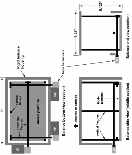
3.5.1 Force balance
Force measurements were done with a force balance designed and built specifically for the GALCIT towing tank by Lisoski (1993). The balance is attached to the underside of the carriage, and, with a special clamp, it suspends the flat plate models vertically in the water (a function it served for all of the experiments). It is capable of resolving time-varying forces on small models at low speeds, yet it can also hold large models and measure forces at high accelerations.
then the output of N1 plus N2, the lift is simply the output of D, and the pitching moment is proportional to N1 minus N2. For the present work, with an angle of attack of 90 degrees, the outputs of N1 and N2 were indistinguishable. Therefore, only the N1 transducer was used, and the drag force was equal to twice the output of N1.
The force balance was calibrated by using a pulley and wire rig to attach a series of known weights to the transducer. Weights were hung on one end of the wire, the other end of which was then run through a pulley and fixed to the load cell. The pulley was needed in order to change the vertical weight into a horizontal force the balance could measure. Lisoski (1993) provides a very thorough treatment of the capabilities and calibration of this particular force balance. The resolution of the force balance, which mechanically amplifies the force on the plate before it reaches the load cells, is ±0.0005 N, equating to a resolution of ±0.02 in the drag coefficient for AR = 6, and ±0.06 for the AR = 2 CD.
3.5.2 Flat plate model clamp
A rotating optical stage was mounted to the center of the measurement platform of the force balance, in order to change the angle of attack of the plate for other studies. Attached to this rotating stage was the model clamp, which was a simple sandwich-style clamp, made from aluminum. The aluminum bracket that fixed the clamp to the optical stage was designed so that the chordline of the plate intersected the center axis of the stage. Since the optical stage was centered on the balance’s measurement platform, centering the plate itself on the stage ensured that no moment arm between the model and the platform (parallel to the plane of measurement) was created.
An Interface model SGA/A strain gage amplifier was used to power the load cell and amplify and filter its output signal. Designed specifically for Interface force transducers, the SGA/A has a large range of output voltage gains, an adjustable low pass filter, adjustable output ranges, and an adjustable offset of up to 79% full-scale in order to “zero” the
transducer. For all force measurements, the load cell excitation was 10 V, the output was set to ±5 V, the gain was set to 17.35, and the low pass filter was set to a cutoff frequency of 5 Hz. This particular gain gave a force transducer output calibration of 0.0023 V/g.
The amplifier output was sent via a breakout board to a PC-mounted data acquisition card, a National Instruments PCI-1200. The PCI-1200 converted the differential analog input into a 12-bit digital signal for the PC. A custom LabVIEW program was written to control the data capturing, including the sampling rate. To avoid picking up the ambient 60 Hz noise in the laboratory, while ensuring that the force balance signal (which included the noise from the drive system) was sampled adequately, a sampling rate of 20 Hz (4 times the 5 Hz cutoff frequency of the amplifier’s low pass filter) was chosen.
3.5.4 Towing tank noise and signal conditioning
frequency of 5 Hz to get rid of the larger magnitude cable noise. The subsequent amplifier output was filtered digitally in Matlab with a cutoff frequency of 2 Hz, which removed the drive system noise while preserving the lower frequency features resulting from the nearly constant kinematics described above. To avoid picking up the ambient 60 Hz noise in the laboratory, while ensuring that the force balance signal was sampled adequately, a sampling rate of 20 Hz was chosen.
Finally, using the experimental procedures described in section 3.2.2, the runs were found to be very repeatable. However, to reduce the impact of the small run-to-run
variations, 10 runs for each aspect ratio were averaged to produce the final force trace.
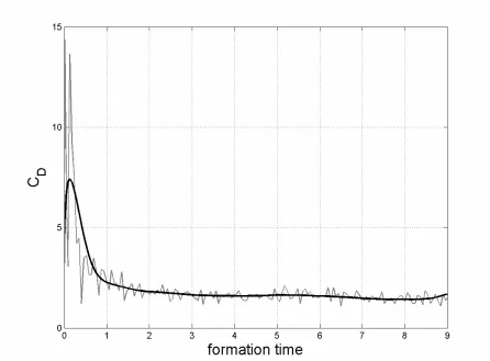
Figure 3.3 CD from amplifier output vs. averaged & digitally filtered CD.
AR = 6, Re = 3000. Gray line: amplifier output from one run;
An example of the amplifier output for a single AR = 6 run (already low-pass filtered with a 5 Hz cutoff frequency) is given by the gray line in Figure 3.3, while the average of all 10 runs, each filtered digitally in Matlab before the averaging, is given by the thicker black line in the same figure.
3.6 DPIV system 3.6.1 DPIV
To capture 2-D sections of the flow velocity quantitatively, and therefore extract quantities such as vorticity, and circulation, digital particle image velocimetry (DPIV) was used. This technique, developed by Willert and Gharib (1991), uses cross-correlation to obtain velocity fields from the displacement of particles between two images separated in time. First, the flow to be interrogated is seeded with particles. Next, a pulsed or chopped laser sheet is used to briefly illuminate an essentially 2-D section of the flow at a periodic rate, and a synchronized video camera then captures a time-sequence of the nearly
instantaneous particle images. Each image in a pair is divided into a set of smaller interrogation windows, which are cross-correlated between the pair to obtain the particle displacement field. Finally, a scaling factor converts the displacement field into the desired velocity field. The computational techniques implemented for the DPIV of the present work are those described in Willert and Gharib (1991) and Westerwheel, Dabiri, and Gharib (1997).
3.6.2 DPIV hardware setup
accomplished using a New Wave Gemini PIV pulsed Nd:YAG laser, which delivered 124 mJ in the 532 nm wavelength per 5 ns pulse. An extremely short duration, high-powered pulse is required so that the captured particle images are essentially instantaneous (or “frozen” in time), but with sufficient luminosity.
As stated in Chapter 2, DPIV data were taken in horizontal (chordwise) planes at three different locations along the plate, 50, 75, and 90% span, as well as in vertical
(spanwise) planes perpendicular to the plate chordline, at mid-chord and at one of the leading edges. The laser beam was spread into an appropriately sized sheet using two identical cylindrical lenses, which could be rotated and leveled so as to produce horizontal or vertical laser sheets. As shown in Figure 3.1, the laser sheet was directed into the tank end closest to the plate. In order to change the height of the horizontal sheets to interrogate different spanwise locations, the head of the Gemini laser, along with the optics, was placed on a height-adjustable pneumatic die table, which could also be rotated to square-up the vertical sheets.
A Pulnix TM-9701 black and white digital CCD video camera, with a resolution of 768 by 480, was used to capture the particle images for DPIV. To image chordwise flow sections, the camera was placed below the tank, looking upward (see Figure 3.1). The camera was mounted on a tripod and pointed at the side of the tank in order to capture the spanwise flow sections. A custom-built timing box synchronized the 30 Hz frame rate of the camera with the laser pulses.
very end of the exposure time for its corresponding video frame, while the laser pulse for the second image in the pair was fired near the very beginning of the exposure time for its, the next, video frame. Thus, the actual time between the pulsed illuminations was much shorter than the full exposure time of one frame (1/30 sec). However, the resulting DPIV velocity fields, one field corresponding to each image pair, were then each separated in time by (1/15 sec). Therefore, the temporal resolution of the overall flow evolution was sacrificed for better temporal resolution of the “instantaneous” flow at each time step; for the moderate Reynolds number of the current investigation, this trade-off was entirely acceptable.
Westerwheel, Dabiri, and Gharib (1997) offer a much more thorough treatment of the subject of time resolution.
3.6.3 DPIV processing
The DPIV processing was done using a 32 by 32 pixel interrogation window, with a 16 by 16 pixel overlap. This gave 48 by 30 (or 1440) vectors for each velocity field, and resulted in a typical resolution, depending upon the imaged section of the flow, of about 7 mm in the horizontal and vertical directions, which was then improved upon using a window shifting technique with the same interrogation window size and overlap (see Westerwheel, Dabiri, & Gharib, 1997). The interrogation window and overlap sizes were chosen so that the number of errant vectors, or outliers, in each velocity field was minimized. The small number of outliers, if any, that appeared in the velocity fields, especially near the plate itself, were removed and replaced by a vector interpolated from its surrounding neighbors via the DPIV software (see Willert & Gharib, 1991).