A Comparison of Computational Efficiencies of Stochastic
Algorithms in Terms of Two Infection Models
H.T. Banks1, Shuhua Hu1, Michele Joyner3
Anna Broido2, Brandi Canter3, Kaitlyn Gayvert4, Kathryn Link5
1
Center for Research in Scientific Computation Center for Quantitative Sciences in Biomedicine
North Carolina State University Raleigh, NC 27695-8212 USA
2
Department of Mathematics Boston College
Chestnut Hill, MA 02467-3806 USA
3
Department of Mathematics and Statistics East Tennessee State University Johnson City, TN 37614-70663 USA
4
Department of Mathematics State University of New York at Geneseo
Geneseo, NY 14454 USA
5
Department of Mathematics Bryn Mawr College Bryn Mawr, PA 19010-2899 USA
May 23, 2012
AMS Subject Classification: 60J27, 60J22, 92D25.
Key Words: Dynamical models, continuous time Markov chain models, stochastic
A Comparison of Computational Efficiencies of Stochastic
Algorithms in Terms of Two Infection Models
Abstract
1
Introduction
Deterministic approaches involving ordinary differential equations to approximate large populations or sample sizes with a continuum, though widely used, have proven less de-scriptive when applied to small populations/sample sizes. To address this issue, contin-uous time Markov chain (CTMC) models are often used when dealing with low species count. There are a variety of stochastic algorithms that can be employed to simulate CTMC models. However, it seems that none of these algorithms can be readily applied to all problems.
The goal of this paper is to illustrate how widely algorithm performances vary be-tween two stochastic infection models and demonstrate how one might perform compu-tational studies to aid in selection of appropriate algorithms. Specifically, we examine three commonly used algorithms: a stochastic simulation algorithm SSA, commonly re-ferred to as the Gillespie algorithm, and explicit and implicit tau-leaping methods. One of our test models is adopted from existing literature, and this model is used to describe Vancomycin-resistant enterococcus (VRE) infection in a hospital unit. The other model is derived in this paper based on an existing deterministic Human Immunodeficiency Virus (HIV) infection model. This new stochastic model is used to describe the dynamics of HIV during the early stage of infection, where the target cells are still at very high numbers while the infected cells are at a very low level.
The methodology illustrated in this paper is highly relevant to current researchers in the biological sciences. As investigations and models of disease progression become
more complex and as interest in initial phases (i.e., HIV acute infection, initial disease
outbreaks) of infections or epidemics increases, the recognition increases that many of these efforts require small population number models (for which ordinary differentail equations (ODEs) are unsuitable). These efforts will involve multiscale discrete valued stochastic models that have as limits (as population numbers increase) ordinary differen-tial equations for the expected population values or means often used (in part because of the ease of their use in simulation studies) in mathematical treatments. As the interest in initial stages of infection grows, so also will the need grow for efficient simulation with these small population numbers models. A major contribution of this paper is a careful presentation of computational issues arising in simulations with such models. A second contribution is the presentation and discussion of a new multiscale discrete stochastic model for HIV infection which in the limit as population numbers increase is an existing clinical-data validated ODE model which has been instrumental in prediction of disease progression and experimental design.
2
Simulation Algorithms
In this section, three computational algorithms for solving stochastic systems will be examined, the stochastic simulation algorithm or Gillespie algorithm, the explicit tau-leaping method and the implicit tau-tau-leaping method. Outlines for implementing each algorithm will be given along with motivations for the algorithm and discussions about when one might want to use one algorithm over another.
Unless otherwise indicated, a capital letter is used to denote a random variable, a bold capital letter is for a random vector, and their corresponding small letters are for their realizations.
2.1
Stochastic Simulation Algorithm
The stochastic simulation algorithm (SSA), also known as theGillespie algorithm[11], is the
standard method employed to simulate continuous time Markov Chain models. The SSA was first introduced by Gillespie in 1976 to simulate the time evolution of the stochas-tic formulation of chemical kinestochas-tics, a process which takes into account that molecules come in whole numbers as well as the inherent degree of randomness in their dynamical behavior. However, in addition to simulating chemically reacting systems, the Gillespie algorithm has become the method of choice to numerically simulate stochastic models arising in a variety of other biological applications [3, 4, 18, 19, 25, 26].
Two mathematically equivalent procedures were originally proposed by Gillespie, the “Direct method” and the “First Reaction method”. Both procedures are exact procedures rigorously based on the chemical master equation [11]; however, the direct method is the method typically implemented due to its efficiency. Likewise, this is the method em-ployed in this paper. The direct method can be described for a general system by
assum-ingX= (X1, X2, ..., Xn)T represents the state variables of the system whereXi(t)denotes
the number in state Xi at time t (Xi may be the number of patients, cells, species, etc).
Furthermore, it is assumedltransitions (often referred to asreaction channelsin
biochem-istry literature) are possible with associated transition rates (often referred to aspropensity
functions in the biochemistry literature) represented by λi, i = 1, ..., l. Given this
termi-nology, the direct method for the Gillespie algorithm can be described by the following procedure:
Step 1. Initialize the state of the systemx0;
Step 2. For the given statexof the system, calculate the transition ratesλi(x),i= 1, ..., l;
Step 3. Calculate the sum of all transition rates,λ=
l
X
i=1
λi(x);
Step 4. Simulate the time,τ, until the next transition by drawing from an exponential
Step 5. Simulate the transition type by drawing from the discrete distribution with
proba-bility Prob(transition=i) =λi(x)/λ. Generate a random numberr2from a uniform
distribution and choose the transition as follows: If0< r2 < λ1(x)/λ, choose
transi-tion 1; ifλ1(x)/λ < r2 <(λ1(x) +λ2(x))/λchoose transition 2, and so on;
Step 6. Update the new timet =t+τ and the new system state;
Step 7. Iterate steps 2-6 untilt≥tstop.
2.2
Tau-Leaping Methods
Since the SSA method keeps track of each transition, it can be impractical to implement for certain applications due to the computational time required. As a result, Gillepsie proposed an approximate procedure, the tau-leaping method, which accelerates the com-putational time while only sustaining a small loss in accuracy [12]. Instead of taking
incremental steps in time, keeping track ofX(t)at each time step as in the SSA method,
the tau-leaping methodleapsfrom one subinterval to the next, approximating how many
transitions take place during a given subinterval. It is assumed that the value of the leap,
τ, is small enough that there is no significant change in the value of the transition rates
along the subinterval [t, t+τ]. This condition is known as the leap condition. The
tau-leaping method thus has the advantage of simulating many transitions in oneleapwhile
not loosing significant accuracy, resulting in a speed up in computational time. In this paper, we consider two tau-leaping methods, an explicit and an implicit version.
2.2.1 An Explicit Tau-Leaping Method
The explicit tau-leaping method is based on an explicit formulation for the update in
number of speciesXat timet+τ, givenX(t) =x. The basic explicit tau-leaping method
approximatesKj, the number of times a transitionj is expected to occur within the time
interval [t, t+τ], by a Poisson random variable Pj(λj(x), τ) with mean (and variance)
λj(x)τ. Once the number of transitions are estimated, the approximate number of species,
known as thetau-leaping approximation, ofXat timet+τ is given by the formula
X(t+τ) = x+ l
X
j=1
Pj(λj(x), τ)vj (2.1)
with vj = (v1j, ..., vnj)T where vij represents the change in state variable Xi caused by
transitionλj [8]. However, as mentioned previously, the process for selectingτ is critical
in the tau-leaping method. If τ is chosen too small, tau-leaping will essentially stop,
leading to the standard SSA algorithm; on the other hand, if the value ofτ is too large,
the leap condition may not be satisfied, possibly causing significant inaccuracies in the
simulation. In this paper, we use a τ-selection procedure based on the algorithm in [8].
Let∆Xi =Xi(t+τ)−xi withxibeing theith component ofx,i = 1,2, . . . n, andbe
an error control parameter with0< 1. In the givenτ-selection procedure,τ is chosen
such that
∆Xi ≤max
gi
xi,1
, i= 1, ..., n, (2.2)
which evidently requires the relative change in Xi to be bounded by
gi
except that Xi
will never be required to change by an amount less than 1. The value of gi in (2.2) is
chosen such that the relative changes in all the transition rates will be bounded by. For
example, if the transition rateλj has the formλj(x) = cjxi withcj being a constant, then
the reactionj is said to be first order and the absolute change inλj(x)is given by
∆λj(x) = λj(x+ ∆x)−λj(x) =cj(xi+ ∆xi)−cjxi =cj∆xi.
Hence, the relative change in λj(x)is related to the relative change in Xi by
∆λj(x)
λj(x)
=
∆xi
xi
, which implies that if we set the relative change in Xi by (i.e., gi = 1), then the
relative change inλj is bounded by. If the transition rateλj has the formλj(x) =cjxixr
withcj being a constant, then the reactionj is said to be second order and the absolution
change inλj(x)is given by
∆λj(x) = cj(xi+ ∆xi)(xr+ ∆xr)−cjxixr=cjxr∆xi+cjxi∆xr+cj∆xi∆xr.
Hence, the relative change inλj(x)is related to the relative change inXiby
∆λj(x)
λj(x)
= ∆xi
xi
+∆xr
xr
+ ∆xi
xi
∆xr
xr
which implies that if we set the relative change inXi by
2 and the relative change inXr
by
2 (i.e., gi = 2, gr = 2), then the relative change inλj is bounded byto the first order
approximation.
The tau-leaping method employed in this paper also includes modifications devel-oped by Cao, et al., [7] to avoid the possibility of negative populations. When utilizing a tau-leaping method instead of the exact SSA method, as discussed previously, estimates are made about how many times a transition has occurred during the leap-interval. From the estimate of the number of transitions and how each transition effects the state
vari-ables, an estimate is obtained for the number of species in each state,Xi, at the end of the
leap-interval. In some instances, if a population or number of species is small at the be-ginning of the leap-interval, the estimate of the state variable after numerous transitions may result in a negative population. To avoid this situation, Cao, et al., [7, 8] introduced
another control parameter,nc, a positive integer (normally set between 2 and 20) which is
A transitionj is deemed critical if afterncof these transitions, there is a danger in one of
the state variables involved in the transition reaching zero. An estimate for the maximum
number of timesLj,j = 1, ..., lthat transitionj can occur before reducing one of the state
variables involved in the transition to 0 (or less) is calculated by
Lj = min
{1≤i≤n;νij<0}
xi
|vij|
with the brackets indicating the floor function. If Lj is less than the control parameter
nc, then the reaction is deemed critical. All critical transitions are then restricted to a
single transition during the leap period reducing the probability of a negative population to nearly zero. All the remaining noncritical transitions use the traditional tau-leaping method. The algorithm for the modified explicit tau-leaping method is given below.
Step 1. Given X(t) = x, identify all critical transitions by first estimating the maximum
number of times,Lj, that a transition can occur before causing a negative population
where
Lj = min
{1≤i≤n;vij<0}
xi
|vij|
with the brackets indicating the floor function. A transition is considered critical if
Lj < nc. (In our calculations, we setnc=10)
Let
Jcr ={j ∈ {1, ..., l}|j is a critical transition}
and
Jncr ={j ∈ {1, ..., l}|j is a noncritical transition}.
Step 2. Choose a value for the error control parameter . (In our calculations, we set =
0.03). Then, compute τ1 so each transition rateλj, j = 1, ..., l is bounded by,
ac-cording to the following definitions:
ˆ
µi(x) =
X
jJncr
vijλj(x), i= 1, ..., n
ˆ
σ2i(x) = X
jJncr
v2ijλj(x), i= 1, ..., n
τ1 = min
{1≤i≤n}
(
max{xi/gi,1}
|µˆi(x)|
,max{xi/gi,1}
2 ˆ
σ2
i(x)
)
(2.3)
wheregi as described in the text.
Step 3. Determine whether tau-leaping is appropriate by comparingτ1 to1/λ. If τ1 is less
than some multiple of1/λ(chosen to be 10 in our calculations), then abandon
Step 4. Compute
λc= X
j∈Jcr
λj(x)
(the sum of all critical transition rates). Generate asecond candidatetime leap,τ2 as a
sample of the exponential random variable with mean1/λc.
Step 5. Letτ = min{τ1, τ2}. Approximate the number of transitions within the time interval,
Kj, as a sample of the Poisson random variable with mean λj(x)τ for allj ∈ Jncr.
For all critical reactions, defineKj as follows:
• Ifτ =τ1, setKj = 0for allj ∈Jcr (no critical transitions occur).
• Ifτ = τ2, let jc be a sample of the integer random variable with point
proba-bilitiesλj(x)/λcforj ∈ Jcr. SetKjc = 1(jcindicates the only critical transition
which occurs) andKj = 0forj ∈Jcr, j 6=jc(only one critical transition occurs).
Step 6. If there is a negative component inx+X
j
Kjvj, reduceτ1by half and return to step
3. Otherwise leap by replacing the time,t = t+τ and the update the new system
state,
x(t+τ) =x+X
j
Kjvj.
Step 7. Iterate steps 1-6 untilt≥tstop.
2.2.2 An Implicit Tau-Leaping Method
In many applications, such as the HIV model explained in Section 3.2, problems of “stiff-ness” may arise. Rathinam et al., [24], explored the nature of stiffness in discrete stochastic systems and demonstrated that an implicit tau-leaping method (similar to implicit Euler methods for ordinary differential equations) is capable of taking large time steps for stiff, discrete systems, producing accurate results for such systems while significantly reduc-ing the computational time when compared to explicit tau-leapreduc-ing methods [14]. The implicit tau-leaping method replaces the explicit update formula given in equation (2.1) by an implicit tau-leaping formula given by
X(t+τ) = x+ l
X
j=1
(Pj(λj(x), τ)−λj(x)τ+λj(X(t+τ))τ)vj,
Note that the above formula typically gives a non-integer vector forX(t+τ). To overcome
this difficulty, Rathinam et al., [24] proposed a two-stage process given by
e
X=x+
l
X
j=1
Pj(λj(x), τ)−λj(x)τ+λj(Xe)τ
and
X(t+τ) = x+ l
X
j=1
r
Pj(λj(x), τ)−λj(x)τ +λj(Xe)τ
z
vj, (2.5)
whereJzKdenotes the nearest non-negative integer corresponding to a real numberz.
The implicit leaping method does not have a stability limitation as the explicit
tau-leaping does (i.e., the relative changes in all the transition rates are bounded by) due to
the implicitness of the scheme. In [9], the stepsize for the stiff system is chosen to bound the relative changes of those transition rates resulting from the non-equilibrium reactions
by, thus, a larger stepsize is allowed. However, as remarked by the authors in [9] that it
is generally difficult to determine whether or not a reaction is in partial equilibrium, and the partial equilibrium condition is only formulated in [9] for those reversible reaction pairs for some biochemical systems. To overcome this difficulty, in this paper we use (2.3)
to choose τ1 for the implicit tau-leaping method but with a larger to allow a possible
large time stepsize.
To avoid the possibility of negative populations (i.e., to ensure (2.4) has non-negative solution), the algorithm for implicit tau-leaping is implemented in the same way as that for the explicit tau-leaping method except the update for states (i.e., replace (2.1) by (2.4) and (2.5)).
3
Biological Applications
In this section, we report on use of the SSA, and the explicit and implicit tau-leaping al-gorithms with two stochastic infection models. One is an existing stochastic model in the literature that is used to describe VRE infection at the population level. The other is derived in this paper based on an existing validated deterministic model for describing the HIV infection within a host. All three algorithms were coded in Matlab, and all the simulation results were run on a Linux machine with a 2GHz Intel Xeon Processor with 8GB of RAM total. We do note that computational times depend on how Matlab codes are written. Hence, all three algorithms are implemented in the same style as well as using similar coding strategies (such as array preallocation and vectorization) to speed up com-putations. Thus the comparison computational times given below should be interpreted as relative to each other for the algorithms discussed rather than in any absolute sense.
The following notation is used throughout the remainder of this paper: Zn is the set
of n-dimensional column vectors with integer components, and ei ∈ Zn is the ith unit
column vector, that is, the ith entry of ei is 1 and all the other entries are zeros, i =
1,2, . . . , n.
form
˜
x=x+
l
X
j=1
[pj−λj(x)τ +λj(˜x)τ]vj, (3.1)
wherepjis the realization ofPj(λj(x), τ). To solve (3.1) forx˜, we first convert the nonlinear
equation (3.1) into the form
g(y) = 0, (3.2)
wherey= (y1, y2, . . . yn)T withx˜ = (y21, y 2
2, . . . , y
2
n) T
, and
g(y) = (y12, y22, . . . , yn2)T −x−
l
X
j=1
pj −λj(x)τ+λj(y12, y
2
2, . . . , y
2
n)τ
vj.
Then we use the commandfsolvein Matlab to obtain the numerical solution of (3.2), and
then the numerical solution for (3.1) is obtained by takingx˜= (y12, y22, . . . , yn2)T. The reason
for converting (3.1) into (3.2) is to avoid possible negative values of state variables.
3.1
A VRE Model
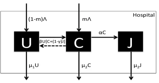
VRE is the group of bacterial species of the genus enterococcus that is resistant to the antibiotic vancomycin, and it can be found in sites such as digestive/gastrointestinal, uri-nary tracts, surgical incision, and bloodstream. The bacteria responsible for VRE can be a member of the normal, usually commensal bacterial flora that becomes pathogenic when they multiply in normally sterile sites. VRE infection is one of the most common infec-tions occurring in hospitals, and this type infection is often referred to as a nosocomial or hospital-acquired infection (these are evidence that hospitals provide not only medical care but also harbor pathogens that pose serious risks of infections).
A stochastic model was developed in [19] to describe the dynamics of VRE infection in a hospital, and it will be used to demonstrate the computational efficiency of the SSA, as well as the explicit and implicit tau-leaping methods. In this model, the patients are
clas-sified as uncolonizedU (those individuals with no VRE present in the body), colonizedC
(those individuals with VRE present in the body) or colonized in isolationJ, as depicted
in the compartmental schematic of Figure 1. From this figure, we see that patients are
admitted into the hospital at a rate ofΛper day, with some fractionmof patients already
VRE colonized (0 ≤ m ≤ 1). Uncolonized patients are discharged from the hospital at
a rate ofµ1U per day, and colonized patients and colonized patients in isolation are
dis-charged from the hospital at rates ofµ2C andµ2J per day, respectively. An uncolonized
patient becomes colonized at a rateβ U[C+ (1−γ)J ] per day, where the hand-hygiene
policy applied to health care workers on isolated VRE colonized patients reduces
infec-tivity by a factor ofγ (0< γ < 1), and the rate of contact is assumed to be proportional to
the population size (i.e., mass action incidence). In addition, a colonized patient is moved
Figure 1: Compartmental VRE Model.
3.1.1 Stochastic VRE Model
In [19], the dynamics of VRE infection are modeled as a continuous time Markov chain. In addition, a constant population is assumed for this model in which the hospital remains full all the time, that is, the overall admission rate equals the overall discharge rate. Let
N denote the total number beds available in the hospital, and{XN(t), t ≥0}be a
contin-uous time Markov chain withXN = (X1N, X2N, X3N)T, where the meaning of the random
variableXiN,i= 1,2,3are given in Table 1.
Variables Description
X1N(t) Number of uncolonized patients at timetin a hospital withN beds
X2N(t) Number of VRE colonized patients at timetin a hospital withN beds
X3N(t) Number of VRE colonized patients in isolation at timetin a hospital withN beds
Table 1: State variables for the VRE model.
In any small time interval of length∆t, we assume{XN(t), t≥0}jumps from statexN
toxN +vj with probabilityλj(xN)∆t+o(∆t), that is,
Prob
XN(t+ ∆t) = xN +vj|XN(t) =xN =λj(xN)∆t+o(∆t), j = 1,2, . . . , l, (3.3)
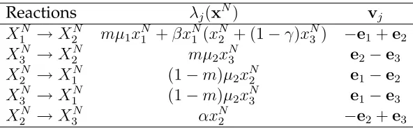
wherexN = (xN1 , xN2 , xN3 )T ∈Z3,vj ∈Z3, andλjis the transition rate for reactionj. Based
on the the assumption of constant population, the transition rates are summarized in the second column of Table 2. From this table, we see that there are five transition rates (i.e,
l = 5), and the corresponding states changesvj are listed in the third column of this table.
Reactions λj(xN) vj
X1N →X2N mµ1xN1 +βx
N
1 (x
N
2 + (1−γ)x
N
3 ) −e1+e2
X3N →X2N mµ2xN3 e2−e3
X2N →X1N (1−m)µ2xN2 e1−e2
X3N →X1N (1−m)µ2xN3 e1−e3
X2N →X3N αxN2 −e2+e3
Table 2: Transition rates λj(xN) as well as the corresponding state changes vj for the
stochastic VRE model (3.3),j = 1,2, . . . ,5.
dependent) CTMC when the sample size is sufficiently large), and this model is given by
˙
UN =−mµ1UN −βUN(CN + (1−γ)JN) + (1−m)µ2CN + (1−m)µ2JN ˙
CN =mµ1UN +βUN(CN + (1−γ)JN) +mµ2JN −(1−m)µ2CN −αCN
˙
JN =−µ2JN +αCN,
(3.4)
whereUN(t),CN(t)andJN(t)denote the number of uncolonized patients, VRE colonized
patients and VRE colonized patients in isolation at timetin a hospital withN beds.
3.1.2 Numerical Results
In this section we report on numerical results obtained by applying the SSA, explicit tau-leaping and implicit tau-tau-leaping methods to the stochastic VRE model (3.3) with transi-tion rates given in Table 2. We compare the computatransi-tional times of the SSA, explicit and
implicit tau-leaping methods with different values ofN. All the simulations were run for
the time period [0, 200] days with parameter values given in the third column of Table 3 and initial conditions (adapted from Table 3 in [19])
XN(0) =N
29 37,
4 37,
4 37
T
, (3.5)
that is, all the simulations start with the same initial density
29 37,
4 37,
4 37
T
.
To implement the tau-leaping methods, we need to find gi, i = 1,2,3. From Table 2
we see that all the reactions are first order except the first one. Let ∆λj(xN) = λj(xN +
∆xN)−λj(xN)with∆xN being the absolute changes in the state variables,j = 1,2, . . . ,5.
Note that
∆λ1(xN) = mµ1∆xN1 +β(x
N
1 + ∆x
N
1 )(x
N
2 + ∆x
N
2 + (1−γ)(x
N
3 + ∆x
N
3 ))
−βxN1 (xN2 + (1−γ)xN3 ) = mµ1∆xN1 +β
xN1 (∆xN2 + (1−γ)∆xN3 ) + ∆xN1 (xN2 + (1−γ)xN3 )
Parameters Description Value
m VRE colonized patient on admission rate 0.04
β Effective contact rate 0.001 per day
γ Hand hygiene compliance rate 0.58
α Patient isolation rate 0.29 per day
µ1 Uncolonized patients discharged rate 0.16 per day
µ2 VRE colonized patients discharge rate 0.08 per day
Table 3: Description of model parameters in the stochastic VRE model as well as the values of parameters used in the simulation.
which implies that
∆λ1(xN)
λ1(xN)
= mµ1∆x
N
1
mµ1xN1 +βxN1 (xN2 + (1−γ)xN3 )
+ βx
N
1 (∆xN2 + (1−γ)∆xN3 )
mµ1xN1 +βxN1 (xN2 + (1−γ)xN3 )
+ β∆x
N
1 (xN2 + (1−γ)xN3 )
mµ1xN1 +βxN1 (xN2 + (1−γ)xN3 )
+ β∆x N
1 (∆xN2 + (1−γ)∆xN3 )
mµ1xN1 +βxN1 (xN2 + (1−γ)xN3 )
.
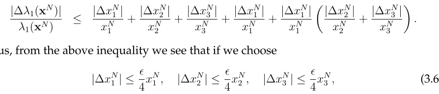
Hence, by the above equation and the positiveness of parameters and non-negativeness of the state variables we have
|∆λ1(xN)|
λ1(xN)
≤ |∆x
N
1 |
xN
1
+|∆x N
2 |
xN
2
+ |∆x N
3 |
xN
3
+ |∆x N
1 |
xN
1
+ |∆x N
1 |
xN
1
|
∆xN
2 |
xN
2
+|∆x N 3 | xN 3 .
Thus, from the above inequality we see that if we choose
|∆xN1 | ≤
4x N
1 , |∆x
N
2 | ≤
4x N
2 , |∆x
N
3 | ≤
4x N
3 , (3.6)
then the relative change in λ1 is bounded by (to the first order approximation). For all
the other first-order reactions, to ensure the relative changes in the transition rates are
bounded by, we need to set the relative changes in the state variables to be bounded by
. Thus, by (3.6) we know that to have|∆λj(xN)| ≤λj(xN)for allj = 1,2, . . . ,5, we need
to set
gi = 4, i= 1,2,3.
For the implicit tau-leaping, the value ofis taken as 0.3 (to allow a possible larger time
stepsize). This value is chosen based on the simulation results so that the computational time is comparatively short without compromising the accuracy of the solution.
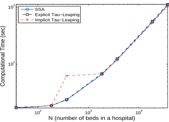
Figure 2 depicts the computational times of each algorithm for an average of five
typ-ical simulation runs with N varying from37,185,370,1850,3700,18500,37000. From this
figure, we see that the computational times for all the algorithms increase as the value
N increases. This is expected for the SSA as the mean time stepsize for the SSA is the
inverse of the sum of all transition rates, which increases as N increases (roughly
102 103 104 101
102
N (number of beds in a hospital)
Computational Time (sec)
SSA
Explicit Tau−Leaping Implicit Tau−Leaping
Figure 2: Comparison of computational times for different algorithms (SSA, Explicit Tau-Leaping and Implicit Tau-Tau-Leaping) for an average of five typical simulation runs.
explicit tau-leaping method we found, for all theN that we tried, the value ofτ1 is often
less than10/λ, which implies that the SSA is implemented most of the time as opposed to
the tau-leaping method (based on the algorithm in Section 2.2.1). This also explains why the SSA and the explicit tau-leaping perform similarly. The same thing is also observed
for the implicit tau-leaping method whenN = 37and 185. However, when N increases
to 370, we found that the implicit tau-leaping method requires significant time for imple-mentation, and we also found that its time stepsize in this case is still not significantly larger than those of the SSA. Note that systems of nonlinear equations must be solved for the implicit tau-leaping method. Hence, the computational time in this case is expected
to be larger than for the other two methods (this can be observed from this figure). AsN
continues increasing, we see that the computational times for the implicit tau-leaping is similar to those of the SSA and the explicit tau-leaping method; this is because the time stepsize becomes significantly larger than those of these two methods in which solving systems of nonlinear equations comprises the main time consuming cost. As one can see
from (2.3) and the transition rates illustrated in Table 2 that if xi/gi > 1 then the first
term inside of the minimum sign of (2.3) is roughly proportional to1/N while the second
term is roughly proportional to 1. The simulation results show that the first term inside
of the minimum sign of (2.3) is smaller than the second term when N increases to 1850
and above. Hence, the time stepsize for the implicit tau-leaping method decreases asN
increases whenN ≥1850, which implies that the computational time for the implicit
tau-leaping method increases as N increases. Based on the above discussions, we see that
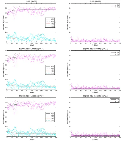
To have some idea on the dynamics of each state variable, we have plotted five typical sample paths of each state of the stochastic VRE model (3.3) obtained by each stochastic algorithm in comparison to the solution for the deterministic VRE model (3.4). Figure 3
depicts the results obtained withN = 37. From this figure, we observe that all the sample
paths for each state variable oscillate around their corresponding deterministic solution, and they exhibit very large differences.
In addition, Figure 3 reveals that the sample paths obtained by the SSA and the
tau-leaping methods exhibit similar variation. The results obtained withN = 370,3700 and
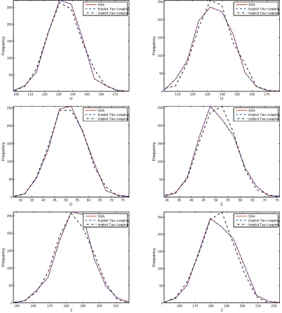
37000 are given in Appendix A. From these figures we also observed that the sample paths obtained by all three algorithms exhibit similar variation. Note that results ob-tained by the SSA are exact. Hence, the difference between histograms obob-tained by the SSA and those obtained by the tau-leaping methods provide a measure of simulation errors in tau-leaping methods when the number of simulation runs are sufficiently large. Thus, to provide further information on the accuracy of the tau-leaping methods, we plot-ted the histograms of state solutions to the stochastic VRE model (3.3) obtained by explicit and implicit tau-leaping algorithms in comparison to those obtained by the SSA. For the
purpose of demonstration, we present here the results only for the case with N = 370.
These histograms are shown in Figure 4 (where plots in the left column are for the
his-tograms of state solutions at t = 80 days, while those in the right column are for the
histograms of state solutions at t = 160days). They were obtained by simulating 1000
sample paths of solutions to the stochastic VRE model. We observe from this figure that the histograms obtained with the explicit tau-leaping algorithm approximately lie on top of those obtained with the SSA, and the histograms obtained with the implicit tau-leaping algorithm are reasonably close to those obtained with the SSA (a similar behavior is also observed for the histograms of state solutions at other time points). This is evidence that the accuracy of results obtained by the tau-leaping methods are reasonably high.
We also observe from Figure 3 as well as those figures in Appendix A that the
vari-ation between the sample paths decreases as N increases, and become quite close to the
deterministic solution whenN = 37000. This agrees with the expectations in light of the
0 20 40 60 80 100 120 140 160 180 200 0 5 10 15 20 25 30 35 40 t (days)
Number of patients
SSA (N=37)
U (D) U (S) J (D) J (S)
0 20 40 60 80 100 120 140 160 180 200 0 5 10 15 20 25 30 35 40 t (days)
Number of patients
SSA (N=37)
C (D) C (S)
0 20 40 60 80 100 120 140 160 180 200 0 5 10 15 20 25 30 35 40 t (days)
Number of patients
Explicit Tau−Leaping (N=37)
U (D) U (S) J (D) J (S)
0 20 40 60 80 100 120 140 160 180 200 0 5 10 15 20 25 30 35 40 t (days)
Number of patients
Explicit Tau−Leaping (N=37)
C (D) C (S)
0 20 40 60 80 100 120 140 160 180 200 0 5 10 15 20 25 30 35 40 t (days)
Number of patients
Implicit Tau−Leaping (N=37)
U (D) U (S) J (D) J (S)
0 20 40 60 80 100 120 140 160 180 200 0 5 10 15 20 25 30 35 40 t (days)
Number of patients
Implicit Tau−Leaping (N=37)
C (D) C (S)
Figure 3: Results in the left column are for uncolonized patients (U) and colonized
pa-tients in isolation (J), and the ones in right column are for the colonized patients (C). The
100 110 120 130 140 150 160 170 50
100 150 200 250
U
Frequency
SSA
Explicit Tau−Leaping Implicit Tau−Leaping
110 120 130 140 150 160 170 0
50 100 150 200 250
U
Frequency
SSA
Explicit Tau−Leaping Implicit Tau−Leaping
30 35 40 45 50 55 60 65 70 75 0
50 100 150 200 250
C
Frequency
SSA
Explicit Tau−Leaping Implicit Tau−Leaping
30 35 40 45 50 55 60 65 70 75 50
100 150 200 250
C
Frequency
SSA
Explicit Tau−Leaping Implicit Tau−Leaping
150 160 170 180 190 200 210 0
50 100 150 200 250
J
Frequency
SSA
Explicit Tau−Leaping Implicit Tau−Leaping
160 170 180 190 200 210 220 0
50 100 150 200 250
J
Frequency
SSA
Explicit Tau−Leaping Implicit Tau−Leaping
Figure 4: Histograms of state solutions to the stochastic VRE model (3.3) att = 80 days
(left column) andt = 160days (right column), where histograms are obtained by
3.2
An HIV Model
HIV is a retrovirus that targets the CD4+ T-cells in the immune system. Once the virus has taken control of a sufficiently large proportion of CD4+ T-cells, an individual is said to have AIDS. There are a wide variety of mathematical models that have been proposed to describe the various aspects of in-host HIV infection dynamics (e.g., [1, 2, 5, 6, 10, 21, 23]). The most basic of these models typically include two or three of the key dynamic compartments: virus, uninfected target cells, and infected cells. These compartmental depictions lead to systems of linear or nonlinear ordinary differential equations in terms of state variables representing the concentrations in each compartment and parameters describing viral production and clearance, cell infection and death rate, treatment efficacy, etc.
The stochastic model we use to demonstrate the computational efficiency of the SSA, and explicit and implicit tau-leaping methods is based on the deterministic HIV model proposed in [5]. Data fitting results validate this model and verify that it provides reason-able fits to all the 14 patients studied. Moreover it has impressive predictive capability when comparing model simulations (with parameters based on estimation procedures using only half of the longitudinal observations) to the corresponding full longitudinal data sets.
3.2.1 Deterministic HIV Model
The model in [5] includes eight compartments: uninfected activated CD4+ T-cells (T1),
uninfected resting CD4+ T cells (T2), along with their corresponding infected states (T1∗
and T2∗), infectious free virus (VI), non-infectious free virus (VN I), HIV-specific effector
CD8+ T-cells (E1), and HIV-specific memory CD8+ T-cells (E2), as depicted in the
com-partmental schematic of Figure 5. In this model, the unit for all the cell compartments is
cells/µl-blood and the unit for the virus compartments is RNA copies/ml-plasma 1. In
addition, protease inhibitor (PI, used to prevent viral replication) and reverse transcrip-tase inhibitor (RTI, used to block new infection) are the two types of drug used to treat HIV patients.
For simplicity, we only consider this model in the case without treatment, and will exclude the non-infectious free virus compartment from the model. In addition, we
con-vert the unit for the free-virus from RNA copies/ml-plasma to RNA copies/µl-blood to
be consistent with the units of cell compartments, and modify the equation based on this change. This conversion will make the derivation of the corresponding stochastic HIV model more direct. With these changes in the model of [5], the state variables and their corresponding units for the deterministic model that we use in this paper is reported in Table 4. The corresponding compartmental ordinary differential equation model is given
1This unit is adopted in [5] because the viral load in the provided clinical data is reported as RNA
Figure 5: Solid gray arrows indicate birth/input. PI and RTI denote protease inhibitors and reverse transcriptase inhibitors, respectively.
States Unit Description
T1 cells/µl-blood concentration of uninfected activated CD4+ T-cells
T1∗ cells/µl-blood concentration of infected activated CD4+ T-cells
T2 cells/µl-blood concentration of uninfected resting CD4+ T-cells
T2∗ cells/µl-blood concentration of infected resting CD4+ T-cells
VI RNA copies/µl-blood concentration of infectious free virus
E1 cells/µl-blood concentration of HIV-specific effector CD8+ T-cells
E2 cells/µl-blood concentration of HIV-specific memory CD8+ T-cells
Table 4: Model states for the deterministic HIV model.
by
˙
T1 =−dT1T1−βT1VIT1−γTT1+nT
aTVI VI+κV +aA
T2,
˙
T1∗ =βT1VIT1−δVT1∗−δEE1T1∗ −γTT1∗+nT
aTVI VI+κV +aA
T2∗,
˙
T2 =ζTVIκs+κs +γTT1−dT2T2−βT2VIT2−
aTVI VI+κV +aA
T2,
˙
T2∗ =γTT1∗ +βT2VIT2−dT2T2∗−
aTVI VI+κV +aA
T2∗,
˙
VI =nVδVT1∗−cVI−(βT1T1 +βT2T2)VI,
˙
E1 =ζE+
bE1T1∗
T∗
1+κb1E1−
dET1∗
T∗
1+κdE1−dE1E1−γE
T1+T1∗
T1+T1∗+κγE1+nE
aEVI VI+κVE2, ˙
E2 =γE
T1+T1∗
T1+T1∗+κγE1+
bE2κb2
E2+κb2E2−dE2E2−
aEVI VI+κVE2,
with an initial condition vector
(T1(0), T1∗(0), T2(0), T2∗(0), VI(0), E1(0), E2(0))T.
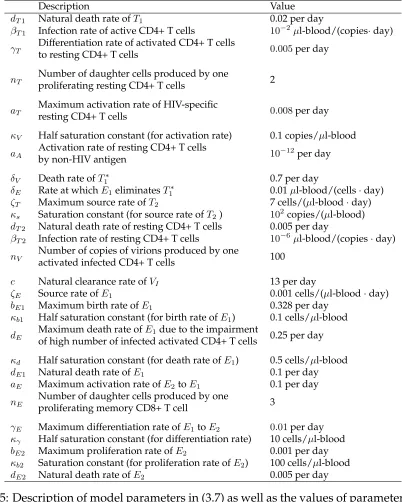
A summary of the description of all the model parameters in (3.7) is given in Table 5. Next we present a brief description of model (3.7), and focus our discussion on the
Description Value
dT1 Natural death rate ofT1 0.02 per day
βT1 Infection rate of active CD4+ T cells 10−2µl-blood/(copies·day)
γT Differentiation rate of activated CD4+ T cells 0.005per day
to resting CD4+ T cells
nT Number of daughter cells produced by one 2
proliferating resting CD4+ T cells
aT Maximum activation rate of HIV-specific 0.008per day
resting CD4+ T cells
κV Half saturation constant (for activation rate) 0.1 copies/µl-blood
aA Activation rate of resting CD4+ T cells 10−12per day
by non-HIV antigen
δV Death rate ofT1∗ 0.7 per day
δE Rate at whichE1eliminatesT1∗ 0.01µl-blood/(cells·day)
ζT Maximum source rate ofT2 7 cells/(µl-blood·day)
κs Saturation constant (for source rate ofT2) 102copies/(µl-blood)
dT2 Natural death rate of resting CD4+ T cells 0.005 per day
βT2 Infection rate of resting CD4+ T cells 10−6µl-blood/(copies·day)
nV Number of copies of virions produced by one 100
activated infected CD4+ T cells
c Natural clearance rate ofVI 13 per day
ζE Source rate ofE1 0.001 cells/(µl-blood·day)
bE1 Maximum birth rate ofE1 0.328 per day
κb1 Half saturation constant (for birth rate ofE1) 0.1 cells/µl-blood
dE Maximum death rate of
E1due to the impairment
0.25 per day of high number of infected activated CD4+ T cells
κd Half saturation constant (for death rate ofE1) 0.5 cells/µl-blood
dE1 Natural death rate ofE1 0.1 per day
aE Maximum activation rate ofE2toE1 0.1 per day
nE Number of daughter cells produced by one 3
proliferating memory CD8+ T cell
γE Maximum differentiation rate ofE1toE2 0.01per day
κγ Half saturation constant (for differentiation rate) 10 cells/µl-blood bE2 Maximum proliferation rate ofE2 0.001 per day
κb2 Saturation constant (for proliferation rate ofE2) 100 cells/µl-blood
dE2 Natural death rate ofE2 0.005 per day
interactions particularly relevant to the derivation of the corresponding stochastic HIV model. The interested readers may refer to [5] for more detailed discussion of the rational behind this model.
The terms dT1T1, dT2T2, dT2T2∗, cVI, dE1E1 +
dET∗
1
T1∗+κdE1 and dE2E2 denote the death (or
clearance) of uninfected activated CD4+ T cells, uninfected resting CD4+ T cells, infected resting CD4+ T cells, infectious free virus, specific activated CD8+ T cells and
HIV-specific memory CD8+ T cells, respectively. The term δEE1T1∗ is used to account for the
elimination of infected activated CD4+ T cells T1∗ by the HIV-specific effector CD8+ T
cells (that is, T1∗ is eliminated from the system at rateδEE1, depending on the density of
HIV-specific effector CD8+ T cells).
The terms involvingβT1VIT1represent the infection process wherein infected activated
CD4+ T cells T1∗ result from encounters between uninfected activated CD4+ T cells T1
and free virus VI (that is, the activated CD4+ T cellsT1 become infected at a rate βT1VI,
depending on the density of infectious virus), and βT2VIT2 is the resulting term for the
infection process wherein infected resting CD4+ T cellsT2∗result from encounters between
uninfected resting CD4+ T cellsT2 and free virusVI (that is, the resting CD4+ T cells T2
become infected at rateβT2VI, depending on the density of infectious virus). In addition,
for simplicity it is assumed that one copy of virion is responsible for one new infection.
Hence, the term (βT1T1+βT2T2)VI in theVI compartment is used to denote the loss of
virions due to infection.
The terms involving γTT1 (resp. γTT1∗) are included in the model to account for the
phenomenon of differentiation of uninfected (resp. infected) activated CD4+ T-cells into
uninfected (resp. infected) resting CD4+ T-cells at rateγT. Similarly, the termγE T1+T
∗
1
T1+T1∗+κγE1
is used to describe the phenomenon of differentiation of HIV-specific activated CD8+ T cells into HIV-specific resting CD8+ T cells.
The termsVIaT+VIκV +aA
T2and
aTVI VI+κV +aA
T2∗represent the activation of uninfected
and infected resting CD4+ T cells, respectively, due to both HIV and some non-HIV
anti-gen. We assume that each proliferating resting CD4+ T cells producenT daughter cells. In
addition, the term VIaEVI+κVE2 denotes the activation of HIV-specific memory CD8+ T cells,
and each proliferating HIV-specific CD8+ T cells producenE daughter cells.
The infected activated CD4+ T cell dies at a rateδV, and producenV copies of virions
during its lifespan (either continuously producing virions during its life or release all its
virions in a single burst simultaneous with its death2).
The termsζTVIκs+κs andζE+
bE1T1∗
T1∗+κb1E1 denote the source rates for the uninfected resting
CD4+ T cells and HIV-specific effector CD8+ T cells, respectively. The term bE2κb2
E2+κb2E2 is
used to account for the self proliferation ofE2(due to the homeostatic regulation).
2For HIV infection, it has not yet been established whether a continuous or burst production model is
3.2.2 The Stochastic HIV Model
In this section, we derive a corresponding stochastic HIV model based on the
determin-istic model (3.7). Letνdenote the volume of blood (in unitsµl-blood), and the parameter
vectorκ= (κV, κs, κb1, κd, κγ, κb2)T whereκV, κs, κb1, κd, κγ, κb2are the saturation constants
in model (3.7). Then we define k = νκ with k = (kV, ks, kb1, kd, kγ, kb2)T, which will be
used in the transition rates for the stochastic model.
Let{Xν(t), t≥0}be a pure jump Markov process withXν = (X1ν, X2ν, . . . , X7ν)T, where
the meanings of random variables Xiν, i = 1,2, . . . ,7are stated as follows. In any small
Variables Description
X1ν(t) number of non-infected activated CD4+ T-cells inν µl-blood at timet
X2ν(t) number of infected activated CD4+ T-cells inν µl-blood at timet
X3ν(t) number of non-infected resting CD4+ T-cells inν µl-blood at timet
X4ν(t) number of infected resting CD4+ T-cells inν µl-blood at timet
X5ν(t) number of RNA copies of infectious free virus inν µl-blood at timet
X6ν(t) number of HIV-specific effector CD8+ T-cells inν µl-blood at timet
X7ν(t) number of HIV-specific memory CD8+ T-cells inν µl-blood at timet
Table 6: State variables for the stochastic HIV model.
time interval of length∆t, we assume that there is only one event (or reaction) that occurs
(e.g., a cell dies, a cell becomes infected, an activated cell is differentiated into a resting
cell, a resting cell becomes activated), and the process{Xν(t), t ≥0}jumps from statexν
toxν +vj with probabilityλj(xν)∆t+o(∆t), that is,
Prob{Xν(t+ ∆t) =xν +vj |Xν(t) =xν}=λj(xν)∆t+o(∆t), j = 1,2, . . . , l, (3.8)
wherexν = (xν1, x2ν, . . . , xν7)T ∈Z7
,vj ∈Z7, andλjis the transition rate for thejth reaction.
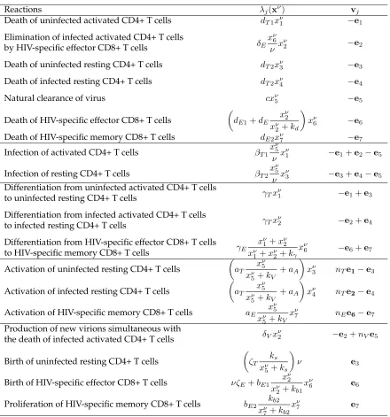
In this stochastic model, we assume a burst production for the viral load (that is, an infected activated CD4+ T cell releases all its virions in a single burst simultaneous with its death). Based on this assumption as well as the discussions in Section 3.2.1, we can obtain the transition rates, which are summarized in the second column of Table 7. From
this table, we see that there are 19 transition rates (i.e., l = 19), and the corresponding
Reactions λj(xν) vj
Death of uninfected activated CD4+ T cells dT1xν1 −e1
Elimination of infected activated CD4+ T cells
δE xν
6
ν x ν
2 −e2
by HIV-specific effector CD8+ T cells
Death of uninfected resting CD4+ T cells dT2xν3 −e3
Death of infected resting CD4+ T cells dT2xν4 −e4
Natural clearance of virus cxν5 −e5
Death of HIV-specific effector CD8+ T cells
dE1+dE xν
2
xν
2+kd
xν6 −e6
Death of HIV-specific memory CD8+ T cells dE2xν7 −e7
Infection of activated CD4+ T cells βT1
xν 5
ν x ν
1 −e1+e2−e5
Infection of resting CD4+ T cells βT2
xν 5
ν x ν
3 −e3+e4−e5
Differentiation from uninfected activated CD4+ T cells γ
Txν1 −e1+e3
to uninfected resting CD4+ T cells
Differentiation from infected activated CD4+ T cells
γTxν2 −e2+e4
to infected resting CD4+ T cells
Differentiation from HIV-specific effector CD8+ T cells γ
E xν
1+xν2
xν1+xν2+kγ
xν6 −e6+e7
to HIV-specific memory CD8+ T cells
Activation of uninfected resting CD4+ T cells
aT xν5
xν
5+kV
+aA
xν3 nTe1−e3
Activation of infected resting CD4+ T cells
aT xν
5
xν5+kV
+aA
xν4 nTe2−e4
Activation of HIV-specific memory CD8+ T cells aE xν
5
xν
5+kV
xν7 nEe6−e7
Production of new virions simultaneous with
δVxν2 −e2+nVe5
the death of infected activated CD4+ T cells
Birth of uninfected resting CD4+ T cells
ζT ks xν
5+ks
ν e3
Birth of HIV-specific effector CD8+ T cells νζE+bE1
xν 2
xν
2+kb1
xν6 e6
Proliferation of HIV-specific memory CD8+ T cells bE2
kb2
xν
7+kb2
xν7 e7
Table 7: Transition rates λj(xν) as well as the corresponding state changes vj for the
stochastic HIV model (3.8).
3.2.3 Numerical Results
In this section, numerical results were obtained by applying the SSA, explicit tau-leaping and implicit tau-leaping methods to the stochastic HIV model (3.8) with transition rates given in Table 7. We compare the computational times of the SSA, explicit and implicit
effectively scales the population counts). Each of the simulations were run for the time period [0, 100] days with parameter values given in the third column of Table 5 (adapted from Table 2 in [5]) and initial conditions
Xν(0) = ν(5,1,1400,1,10,5,1)T. (3.9)
That is, each of the simulations start with the same initial concentrations(5,1,1400,1,10,5,1)T.
To implement the tau-leaping methods, we need to findgi,i= 1,2, . . . ,7. From Table 7
we see that all the reactions are either zero order, or first order or second order. However,
a lot of them have transition rates with non-constant coefficients (λ6,λ12,λ13,λ14,λ15,λ17,
λ18, λ19). For these reactions,gi is not just one or two. Here we will take reaction six as
an example to illustrate this. Let ∆λi(xν) = λi(xν + ∆xν)−λi(xν)with ∆xν being the
absolute changes in the state variables,i= 1,2, . . . ,19. Note that
∆λ6(xν) = dE1∆xν6+dE
(xν
2 + ∆xv2)(xν6 + ∆xv6)
xν
2 + ∆xv2 +kd
− x
ν
2xν6
xν
2+kd
=dE1∆xν6
+ dE [xν
2xν6 +xν2∆xν6 +xν6∆xν2+ (∆xν2)(∆x6ν)](xν2 +kd)−xν2xν6(xν2+ ∆xv2+kd) (xν
2 + ∆xv2 +kd)(xν2 +kd) = dE1∆xν6+dE
[xν
2∆xν6 +xν6∆xν2+ (∆xν2)(∆x6ν)](xν2 +kd)−xν2xν6∆xv2 (xν
2 + ∆xv2 +kd)(xν2 +kd) = dE1∆xν6+dE
xν
2(xν2 +kd)∆xν6+kdxν6∆xν2+ (xν2 +kd)∆xν2∆xν6 (xν
2 + ∆xv2+kd)(xν2 +kd)
,
which implies that
∆λ6(xν)
λ6(xν)
= dE1∆x ν
6
dE1xν6+dE
xν
2xν6
xν
2+kd
+
dE
xν
2(xν2+kd)∆xν6+kdxν6∆xν2+(xν2+kd)∆xν2∆xν6 (xν
2+∆xv2+kd)(xν2+kd)
dE1xν6 +dE
xν
2xν6
xν
2+kd
Thus, by the above equation as well as the non-negativeness of the state variables and the positiveness of the parameters we have
|∆λ6(xν)|
λ6(xν)
< |∆x
ν 6| xν 6 + xν
2(xν2+kd)∆xν6 +kdxν6∆xν2 + (xν2 +kd)∆xν2∆xν6 (xν
2 + ∆xv2 +kd)xν2xν6
≤ |∆x
ν 6| xν 6 + x ν
2 +kd
|xν
2 + ∆xv2+kd|
|∆xν
6|
xν
6
+ kd
|xν
2+ ∆xv2+kd|
|∆xν
2|
xν
2
+ x
ν
2 +kd
|xν
2 + ∆xv2+kd|
|∆xν2|
xν
2
|∆xν6|
xν
6
.
(3.10)
If the value ofis set to be < 1
2, we find|∆x
ν
i| ≤ixνi ≤ 1 2(x
ν
i +kd), which implies that
xν2 +kd
|xν
2 + ∆xv2+kd|
≤ 1
2,
kd
|xν
2 + ∆xv2+kd|
Hence, by (3.2.3) and the above inequality we obtain
|∆λ6(xν)|
λ6(xν)
<3|∆x
ν
6|
xν
6
+|∆x ν
2|
xν
2
+ 2|∆x ν
2|
xν
2
|∆xν
6|
xν
6
.
Thus, from the above inequality we see that if we choose
|∆xν6| ≤
4x ν
6, |∆x
ν
2| ≤
4x ν
2, (3.11)
then the relative change inλ6 is bounded by(to the first order approximation). Similarly
to have the relative changes in the other transition rates with non-constant coefficient to
be bounded by(either exactly or to the first order approximation), we need to set
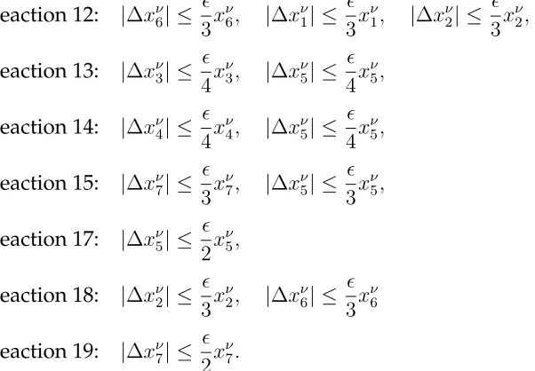
Reaction 12: |∆xν6| ≤
3x ν
6, |∆x
ν
1| ≤
3x ν
1, |∆x
ν
2| ≤
3x ν
2,
Reaction 13: |∆xν3| ≤
4x ν
3, |∆x
ν
5| ≤
4x ν
5,
Reaction 14: |∆xν4| ≤
4x ν
4, |∆x
ν
5| ≤
4x ν
5,
Reaction 15: |∆xν7| ≤
3x ν
7, |∆xν5| ≤
3x ν
5,
Reaction 17: |∆xν5| ≤
2x ν
5,
Reaction 18: |∆xν2| ≤
3x ν
2, |∆x
ν
6| ≤
3x ν
6
Reaction 19: |∆xν7| ≤
2x ν
7.
(3.12)
For those transition rates with constant coefficient, we can easily see that to have them be
bounded by(to the first order approximation) we need to set the relative changes in the
state variables to be bounded by either 1
2 (to those second order reaction) or(to those
first order reaction). Thus, by (3.11) and (3.12) we know that to have |∆λi| ≤ λi for all
i= 1,2, . . . ,19, we need to set
gi =
(
4, i= 2,3,4,5,6
3, i= 1,7.
For the implicit tau-leaping method, was taken as 0.12 (to allow a larger time
step-size). This value is chosen based on the simulation results so that the computational time is comparatively short without compromising the accuracy of the solution.
Figure 6 depicts the computational time of each algorithm for an average of five
101 102 103 104 105 106 101
102 103 104
νµl−blood
Computational Time (sec)
SSA
Explicit Tau−Leaping Implicit Tau−Leaping
Figure 6: Comparison of computational times of different algorithms (SSA, Explicit Tau-Leaping and Implicit Tau-Tau-Leaping) for an average of five typical simulation runs.
10,50,102,2×102,5×102,103,104,105,106,5×106for the explicit and implicit tau-leaping
schemes. From this figure, we see that the computational times for the SSA increase as
the valueν increases. This is again expected as the mean time stepsize for the SSA is the
inverse of the sum of all transition rates, which increases asνincreases (roughly
propor-tional to ν, as can be seen from the transition rates illustrated in Table 7). In addition,
even withν = 103, it took the SSA more than8000seconds for one sample path (which is
why we did not run any simulations for the SSA whenν is greater than103). Hence, it is
impractical to implement the SSA if we want to run this HIV model for a normal person
(generally having approximately5×106µl-blood). This is expected due to the large value
of uninfected resting CD4+ T cells (as can be seen from the initial condition (3.9)).
From Figure 6 we also see that the computational times for the explicit tau-leaping
method increase as the valueνincreases from 10 to 50, and decrease asνincreases to 100.
Then its computational times decrease dramatically as the value ofν increases from 100
to104, and stabilizes somewhat forν ≥ 104. This is due in some way to the formula for
τ1. As we can see from (2.3) and transition rates in Table 7 that ifxi/gi >1then the first
term inside the minimum sign of (2.3) is roughly in the same order for all the values of
ν while the second term is roughly proportional to the value ofν. In addition, we found
from the simulation results that the first term inside the minimum sign of (2.3) is much
larger than the corresponding second term until ν = 104, and becomes smaller than the
second term when ν ≥ 104. Hence, τ1 increases as ν increases whenν ≤ 104 and has
roughly similar values for all the cases whenν ≥ 104, which agrees with the observation
that the computational times decrease dramatically as the value of ν increases from 100
to104, and stabilizes there forν ≥104. The increase of computational times asνincreases
instead of tau-leaping.
We also observe from Figure 6 that the computational times for the implicit tau-leaping
method decrease asν increases whenν ≤ 104 and then stabilizes there forν ≥ 104. This
is for the same reason as that for the explicit tau-leaping method. In addition, we see that the computational times for the implicit tau-leaping is significantly higher than those
of the SSA and the explicit tau-leaping at ν = 10, which is because under this case the
implicit tau-leaping is implemented many times (solving systems of nonlinear equations in each implicit tau-leaping step is costly) and the time stepsize is not significantly larger than those of the other two methods.
Based on the above discussions, we know that for smaller values of ν (less than 100)
the SSA is the choice due to its simplicity, accuracy and efficiency. However, for larger values the tau-leaping methods are definitely the choice with implicit tau-leaping per-forming better than explicit tau-leaping; this is expected due to the stiffness of the system (large variations in both parameter values and state variables).
To have some idea on the dynamics of each state variable, we plotted five typical sample paths of solution to stochastic HIV model (3.8) (in terms of concentrations, i.e.,
Xν(t)/ν) obtained by each stochastic algorithm in comparison to the solution for the
de-terministic HIV model (3.7). Figures 7-8 depict the results obtained withν = 10µl-blood,
where the results in Figure 7 are for CD4+ T cells, and the ones in Figure 8 are for the infectious virus and CD8+ T cells. The right column of Figure 7 reveals that all the
sam-ple paths for the uninfected resting CD4+ T cells (T2) are similar to their corresponding
deterministic solutions, which is expected as the value of the uninfected resting CD4+ T cells is so large that its dynamics can be well approximated by the ordinary differential equation. While all the other state variables oscillate around their corresponding deter-ministic solution (as can be seen from these two figures), and the variations of the sample
paths for the infectious virus (VI) and CD8+ T cells (E1 andE2) are especially large. This
is expected asT2 has less effect on the dynamics of these three compartments (especially
onE1andE2, as observed from (3.7) and the parameter values in Table 5).
In addition, Figures 7 and 8 reveal that the sample paths obtained by the SSA and the tau-leaping methods exhibit similar variation, which suggests that tau-leaping meth-ods have reasonably high accuracy. The results obtained by all three algorithms with ν = 100,1000µl-blood are given in Appendices B.1 and B.2, and the results obtained by
the tau-leaping methods withν = 104,105 and 5×10⁶ are given in Appendices B.3-B.5.
From the figures in Appendices B.1 and B.2 we observe that the sample paths obtained by all three algorithms exhibit similar variation, and the variation between the sample paths
decreases asνincreases. The same conclusion can be obtained from the figures in
Appen-dices B.3-B.5. To gain further information on the accuracy of the tau-leaping methods, we plotted the histograms of state solutions to the stochastic HIV model (3.8) (in terms of concentration) obtained by explicit and implicit tau-leaping methods in comparison to those obtained by the SSA. Due to long computational times to obtain these histograms,
we present here the results only for the case withν = 200µl-blood (where computational
0 10 20 30 40 50 60 70 80 90 100 10−1 100 101 102 t (days)
Activated CD4+ T cells (cells/
µ
l−blood)
SSA (ν=10)
T1 (D) T
1 (S)
T1* (D) T1* (S)
0 10 20 30 40 50 60 70 80 90 100 10−1 100 101 102 103 104 t (days)
Resting CD4+ T cells (cells/
µ
l−blood)
SSA (ν=10)
T2 (D) T
2 (S)
T2* (D) T2* (S)
0 10 20 30 40 50 60 70 80 90 100 10−1
100 101 102
t (days)
Activated CD4+ T cells (cells/
µ
l−blood)
Explicit Tau−Leaping (ν=10)
T
1 (D)
T1 (S) T1* (D) T1* (S)
0 10 20 30 40 50 60 70 80 90 100 10−1 100 101 102 103 104 t (days)
Resting CD4+ T cells (cells/
µ
l−blood)
Explicit Tau−Leaping (ν=10)
T
2 (D)
T2 (S) T2* (D) T2* (S)
0 10 20 30 40 50 60 70 80 90 100 10−1
100 101 102
t (days)
Activated CD4+ T cells (cells/
µ
l−blood)
Implicit Tau−Leaping (ν=10)
T
1 (D)
T1 (S) T1* (D) T
1 * (S)
0 10 20 30 40 50 60 70 80 90 100 10−1 100 101 102 103 104 t (days)
Resting CD4+ T cells (cells/
µ
l−blood)
Implicit Tau−Leaping (ν=10)
T
2 (D)
T2 (S) T2* (D) T
2 * (S)
Figure 7: Results for uninfected and infected activated CD4+ T cells (left column), and uninfected and infected resting CD4+ T cells (right column). The (D) and (S) in the leg-end denote the solution obtained by the deterministic HIV model and the stochastic HIV model, respectively, where the stochastic results are obtained by the SSA (top two pan-els), the explicit tau-leaping (middle two panels) and the implicit tau-leaping (bottom two panels).
0 10 20 30 40 50 60 70 80 90 100 10−1
100 101
102 103
t (days)
Infectious free virus (RNA copies/
µ
l−blood)
SSA (ν=10)
VI (D) VI (S)
0 10 20 30 40 50 60 70 80 90 100 10−1
100
101 102
t (days)
HIV specific CD8+ T cells (cells/
µ
l−blood)
SSA (ν=10)
E1 (D) E1 (S) E
2 (D)
E2 (S)
0 10 20 30 40 50 60 70 80 90 100 10−1
100 101
102 103
t (days)
Infectious free virus (RNA copies/
µ
l−blood)
Explicit Tau−Leaping (ν=10)
VI (D) VI (S)
0 10 20 30 40 50 60 70 80 90 100 10−1
100 101 102
t (days)
HIV specific CD8+ T cells (cells/
µ
l−blood)
Explicit Tau−Leaping (ν=10)
E1 (D) E1 (S) E
2 (D)
E2 (S)
0 10 20 30 40 50 60 70 80 90 100 10−1
100 101
102 103
t (days)
Infectious free virus (RNA copies/
µ
l−blood)
Implicit Tau−Leaping (ν=10)
VI (D) VI (S)
0 10 20 30 40 50 60 70 80 90 100 10−1
100 101 102
t (days)
HIV specific CD8+ T cells (cells/
µ
l−blood)
Implicit Tau−Leaping (ν=10)
E1 (D) E1 (S) E
2 (D)
E2 (S)
Figure 8: Results for infectious virus (left column), and HIV-specific CD8+ T cells (right column). The (D) and (S) in the legend denote the solutions obtained by the deterministic HIV model and the stochastic HIV model, respectively, where the stochastic results are obtained by the SSA (top two panels), the explicit tau-leaping (middle two panels) and the implicit tau-leaping (bottom two panels).
model. The plots in Figure 9 are for histograms of state solutions at t = 50 days, and
those in Figure 10 are for histograms of state solutions att = 100days. We observe from
close to those obtained by the SSA (similar behavior is also observed for the histograms of state solutions at other time points). This suggests that the accuracy of results obtained by tau-leaping methods are acceptable (recall that results obtained by the SSA are exact, so the differences between histograms obtained by the SSA and the ones obtained by tau-leaping methods provide a measure of simulation errors in tau-tau-leaping methods when the number of simulation runs is sufficiently large).
We also observe from the figures in Appendix B.5 that the stochastic solutions agree
with the deterministic solutions whenν = 5×10⁶ µl-blood. This suggests that ordinary
12.5 13 13.5 14 14.5 15 15.5 0
50 100 150 200 250 300
T1
Frequency
SSA Explicit Tau−Leaping Implicit Tau−Leaping
16.5 17 17.5 18 18.5 19 19.5 0
50 100 150 200 250
T1*
Frequency
SSA Explicit Tau−Leaping Implicit Tau−Leaping
848 850 852 854 856 858 0
50 100 150 200 250
T2
Frequency
SSA Explicit Tau−Leaping Implicit Tau−Leaping
8.4 8.6 8.8 9 9.2 9.4 9.6 0
50 100 150 200 250
T2*
Frequency
SSA Explicit Tau−Leaping Implicit Tau−Leaping
80 85 90 95 100 105 110 0
50 100 150 200 250
VI
Frequency
SSA Explicit Tau−Leaping Implicit Tau−Leaping
4 4.5 5 5.5 6 6.5 7 7.5 8 8.5 9 0
50 100 150 200 250
E1
Frequency
SSA Explicit Tau−Leaping Implicit Tau−Leaping
0.25 0.3 0.35 0.4 0.45 0.5 0.55 0.6 0.65 0
50 100 150 200
E 2
Frequency
SSA Explicit Tau−Leaping Implicit Tau−Leaping
Figure 9: Histograms of state solutions to the stochastic HIV model (3.8) (in terms of
concentrations) with ν = 200 µl-blood att = 50 days, where histograms are obtained by
12.5 13 13.5 14 14.5 15 15.5 0
50 100 150 200 250
T 1
Frequency
SSA Explicit Tau−Leaping Implicit Tau−Leaping
11.5 12 12.5 13 13.5 50
100 150 200 250
T 1 *
Frequency
SSA Explicit Tau−Leaping Implicit Tau−Leaping
588 590 592 594 596 598 0
50 100 150 200 250
T2
Frequency
SSA Explicit Tau−Leaping Implicit Tau−Leaping
8.8 9 9.2 9.4 9.6 9.8 10 50
100 150 200 250
T2*
Frequency
SSA Explicit Tau−Leaping Implicit Tau−Leaping
55 60 65 70 75 80 0
50 100 150 200 250 300
V I
Frequency
SSA Explicit Tau−Leaping Implicit Tau−Leaping
3 4 5 6 7 8 9 10 50
100 150 200 250
E 1
Frequency
SSA Explicit Tau−Leaping Implicit Tau−Leaping
0.2 0.3 0.4 0.5 0.6 0.7 0.8 0
50 100 150 200 250
E 2
Frequency
SSA Explicit Tau−Leaping Implicit Tau−Leaping
Figure 10: Histograms of state solutions to the stochastic HIV model (3.8) (in terms of
concentrations) withν = 200µl-blood att= 100days, where histograms are obtained by
4
Concluding Remarks
In this paper we present a detailed discussion on how to apply the tau-leaping methods to two stochastic infection models with different levels of complexity, and compared their computational efficiency along with that of the SSA. One of these models is an existing stochastic model used for describing the dynamics of VRE infection in a hospital unit. The other model is derived in this paper based on an existing deterministic model used for describing the dynamics of HIV infection within a host.
Even though tau-leaping methods have now been widely used in biochemistry litera-ture, to our knowledge, tau-leaping methods have not been applied to complex nonlinear dynamical infectious disease models such as the HIV model that we presented in this pa-per (with transition rates being complicated nonlinear functions of state variables rather than some simple polynomial functions). We do note that the computational performance of these three methods vary from model to model (as we demonstrated in this paper), which suggests that for a given model of interest one might need to perform some initial simulation studies to select an appropriate algorithm (for example among those we pro-pose in this paper). However, the step-by-step implementation recipe demonstrated in this paper for these algorithms can be applied to a wide range of other complex biologi-cal models, specifibiologi-cally those in infectious disease progression and epidemics.
Simulation results reveal that for both models the computational times of the SSA
increase as the sample size (number of beds N in the VRE model and volume of blood
ν in the HIV model) increases. This is because the mean time stepsize for the SSA is the
inverse of the sum of transition rates, which increases as the sample size increases. In addition, the results suggest all three algorithms have comparable computational times for the VRE model because of the low number of species and small number of transitions, and the SSA is the best choice for this problem due to its simplicity and accuracy. For the HIV model both tau-leaping methods have significantly lower computational costs
than those of the SSA except when the sample size ν is very small (e.g., less than 100
µl-blood). In addition, the implicit tau-leaping method has lower computational costs than the explicit tau-leaping method when the sample size is sufficiently large (due to the stiffness of the system).
Note that the stochastic HIV model in this paper is of interest in early or acute infec-tion where the number of uninfected resting T cells is large (on the order of 1000 cells per µl-blood). This explains why the SSA requires more than 8000 seconds to run even one
sample path withν = 1000µl-blood. If one considers an average person having5×106
µl-blood, to run the SSA for even one sample path is impractical at this scale. The numerical results demonstrate the dynamics of uninfected resting CD4+ T cells can be well
approx-imated by ordinary differential equations even withν = 10 µl-blood. In addition, Table
sub-systems, one containing fast reactions and the other containing slow reactions. Then the two subsystems are simulated