Zurich Open Repository and Archive University of Zurich Main Library Strickhofstrasse 39 CH-8057 Zurich www.zora.uzh.ch Year: 2016
Determination of target detection limits in hyperspectral data using band
selection and dimensionality reduction
Gross, Wolfgang ; Böhler, Jonas ; Twizer, Kfir ; Kedem, Bar ; Lenz, Andreas ; Kneubühler, Mathias ; Wellig, Peter ; Oechslin, Roland ; Schilling, Hendrik ; Rotman, Stanley R ; Middelmann, Wolfgang
Abstract: Hyperspectral remote sensing data can be used for civil and military applications to robustly detect and classify” ”target objects. High spectral resolution of hyperspectral data can compensate for the comparatively low spatial resolution, which allows for detection and classification of small targets, even below image resolution. Hyper- spectral data sets are prone to considerable spectral redundancy, affecting and limiting data processing and algorithm performance. As a consequence, data reduction strategies become increasingly important, especially in view of near-real-time data analysis. The goal of this paper is to analyze different strategies for hyperspectral band selection algorithms and their effect on subpixel classification for different target and background mate- rials. Airborne hyperspectral data is used in combination with linear target simulation procedures to create a representative amount of target-to-background ratios for evaluation of detection limits. Data from two different airborne hyper-spectral sensors, AISA Eagle Hawk, are used to evaluate transferability of band selection when using different sensors. The same target objects were recorded to compare the calculated detection limits. To determine subpixel classification results, pure pixels from the target materials are extracted and used to simulate mixed pixels with selected background materials. Target signatures are linearly combined with different back- ground materials in varying ratios. The commonly used classification algorithms Adaptive Coherence Estimator (ACE) is used to compare the detection limit for the original data with several band selection and data reduction strategies. The evaluation of the classification results is done by assuming a fixed false alarm ratio and calcu- lating the mean target-to-background ratio of correctly detected pixels. The results allow drawing conclusions about specific band combinations for certain target and background combinations. Additionally, generally useful wavelength ranges are determined and the optimal amount of principal components is analyzed.
DOI: https://doi.org/10.1117/12.2240931
Posted at the Zurich Open Repository and Archive, University of Zurich ZORA URL: https://doi.org/10.5167/uzh-127374
Conference or Workshop Item Published Version
Originally published at:
Gross, Wolfgang; Böhler, Jonas; Twizer, Kfir; Kedem, Bar; Lenz, Andreas; Kneubühler, Mathias; Wellig, Peter; Oechslin, Roland; Schilling, Hendrik; Rotman, Stanley R; Middelmann, Wolfgang (2016). Determi-nation of target detection limits in hyperspectral data using band selection and dimensionality reduction. In: Target and Background Signatures II, Edinburgh, 26 September 2016 - 27 September 2016, 99970H. DOI: https://doi.org/10.1117/12.2240931
Determination of target detection limits in hyperspectral
data using band selection and dimensionality reduction
Gross W.
a, Boehler J.
b, Twizer, K.
c, Kedem, B.
c, Lenz, A.
a, Kneubuehler M.
b, Wellig P.
d,
Oechslin R.
d, Schilling, H.
a, Rotman, S.
c, and Middelmann W.
aa
Fraunhofer Institute of Optronics, System Technologies and Image Exploitation IOSB,
Gutleuthausstrasse 1, D-76275 Ettlingen, Germany;
b
Remote Sensing Laboratories, University of Zurich, Winterthurerstrasse 190, CH-8057 Zurich,
Switzerland;
c
Department of Electrical & Computer Engineering, Ben-Gurion University, Be’er-Sheba,
Israel;
d
Science and Technology Department, armasuisse, Feuerwerkerstasse 39, CH-3602 Thun,
Switzerland
ABSTRACT
Hyperspectral remote sensing data can be used for civil and military applications to robustly detect and classify target objects. High spectral resolution of hyperspectral data can compensate for the comparatively low spatial resolution, which allows for detection and classification of small targets, even below image resolution. Hyper-spectral data sets are prone to considerable Hyper-spectral redundancy, affecting and limiting data processing and algorithm performance. As a consequence, data reduction strategies become increasingly important, especially in view of near-real-time data analysis. The goal of this paper is to analyze different strategies for hyperspectral band selection algorithms and their effect on subpixel classification for different target and background mate-rials. Airborne hyperspectral data is used in combination with linear target simulation procedures to create a representative amount of target-to-background ratios for evaluation of detection limits. Data from two different airborne hyperspectral sensors, AISA Eagle & Hawk, are used to evaluate transferability of band selection when using different sensors. The same target objects were recorded to compare the calculated detection limits. To determine subpixel classification results, pure pixels from the target materials are extracted and used to simulate mixed pixels with selected background materials. Target signatures are linearly combined with different back-ground materials in varying ratios. The commonly used classification algorithms Adaptive Coherence Estimator (ACE) is used to compare the detection limit for the original data with several band selection and data reduction strategies. The evaluation of the classification results is done by assuming a fixed false alarm ratio and calcu-lating the mean target-to-background ratio of correctly detected pixels. The results allow drawing conclusions about specific band combinations for certain target and background combinations. Additionally, generally useful wavelength ranges are determined and the optimal amount of principal components is analyzed.
Keywords: Hyperspectral, detection limit, target-to-background ratio, band selection, subpixel, simulation, target detection, dimensionality reduction
1. INTRODUCTION
In 2015 we published an approach to approximate the subpixel target detection limits in hyperspectral data in Gross et al.1 Multiple commonly used classifiers were analyzed, e.g. Spectral Angular Mapper (SAM),2
Matched Filter (MF),3 Adaptive Coherence Estimator (ACE)3 and Orthogonal Subspace Projection (OSP).3
Real hyperspectral data from aisaEagle (VNIR) & aisaHAWK (SWIR) was used together with simulated target-to-background ratios. The target and background spectra were taken directly from the scene to prevent the introduction of different statistical properties into the data. All available bands were used, 127 bands for
Send correspondence to W. Gross E-mail: [email protected]
VNIR and 235 bands for SWIR. The results were given as the target fraction at 0.1 % false alarms. For some target/background combinations a mean target fraction of 5 % was sufficient in the original data. This leads to the question, if a clever selection of bands can improve the results as stated by Yu et al.4
The goal is to eliminate or mitigate bands that contain no useful information, e.g. due to atmospheric absorptions or redundant information. Since we are also evaluating different target and background combinations, evaluating the results for similar bands is done to check for valuable bands that can be used for more than one combination.
For this paper, two bandselection methods are evaluated. The methods areForward Selection with Internal and External Clustering and Backwards Elimination with Internal Clustering. For evaluation the same aisaEAGLE & aisaHAWK data from our previous paper is used.1
In section 2 the bandselection and evaluation procedures are explained. Section 3 describes the measurement campaign and the data simulation process. The evaluation takes place in section 4.
2. OBJECTIVE AND BANDSELECTION METHODS
The scope of this paper are the following objectives:• Perform bandselection: Forward Selection with Internal and External Clustering and Backwards Elimina-tion with Internal Clustering
• Evaluate results for detection limit of subpixel targets
• Compare results of two different sensor systems on identical target/background combinations • Compare results for ’universally’ valuable band combinations
To introduce the bandselection methods it is important to keep in mind that each selection is calculated with a specific target and background signature in mind. Real hyperspectral remote sensing data is used as input data. Linear mixtures of specific target and background spectra taken from these data sets, are appended to the data sets to generate spectra with known mixture ratios. In the next step bands are iteratively selected/eliminated or clustered by evaluating the classification results of ACE. Internal clustering refers to calculating the weighted mean of bands that were already selected. External clustering is a weighted clustering where at least one previously unused band is introduced.
We use the following notation to describe the bandselection algorithms and the ACE classifier:
LetV ∈Rn×N be the hyperspectral data set withn spectral bands and N samples. As neither bandselection nor classification requires neighborhood information we are able to reorganize the 3D data cube such that matrix operations are possible. Lets∈Rn be the n-dimensional vector of the spectral target signature andx∈Rn be a sample spectrum from the data setV. Σ∈Rn×n is the covariance matrix ofV, also referred to as background covariance matrix as we removed all target areas from the data to not disturb the statistics. Finally,µ∈Rn is the mean spectral signature ofV andes=s−µandxe=x−µare the centralized target and sample vectors. ACE classification assumes knowledge of background statistics in the form of a covariance matrix Σ. ACE has the property of constant false alarm rate (CFAR), which implies that the probability of false alarm is independent of background covariance matrix. The calculation is done by
ACE(x) = es TΣ−1 e x2 (esTΣ−1 e s) (xeTΣ−1 e x).
It is invariant to relative scaling of test and training data. ACE was chosen in this paper since it achieved the best results in a majority of cases in Gross et al.1
The output of each ACE iteration is a similarity value per sample x. A subsequent binary classification can be done by a nearest neighbor approach when more than one target is used. In our case only one target signature is used at a time and a threshold to the similarity images is applied to enforce a desired false alarm rate.
2.1 Forward Selection with Internal and External Clustering
The first among the analyzed methods is an iterative procedure. LetV ∈Rn×N be the original data set with
n bands. During each iteration either a new band is selected from the number of previously unused bands and added to the bandselection data setV ∈Rt×N,t≤p≤n, or two neighboring bands are clustered. The following steps are performed during each iteration:
1. Select a band ofV that is not yet included inV. Temporarily add this band toV and calculate classification results. Do this for all eligible bands and save index of the best result.
2. Calculate the weighted mean for each pair of already selected bands/clusters and their direct neighbor and calculate classification results. The weights are determined by the sum of bands in each cluster. Save the combination giving the best result.
3. Determine the action that gives the best result from previous steps. If step 1 was best, add that specific band to the bandselection dataVold∈Rt×N ⇒Vnew ∈Rt+1×N. If step 2 was best, cluster the best band
combination and replace these bands. For external clustering Vold∈Rt×N ⇒Vnew ∈Rt×N, for internal
clusteringVold∈Rt×N ⇒Vnew ∈Rt−1×N.
4. Repeat steps 1–3 until a termination condition is met, e.g. a fixed number of selection/clustering operations was performed or the dimension of the data set isV ∈Rp×N with predefinedp.
2.2 Backward Elimination with Internal Clustering
The second method is also an iterative procedure. This approach starts with the whole original data setV and eliminates a band or clusters neighboring bands in each step. The algorithm can be described similar toForward Selection with Internal and External Clustering by:
1. Select a band of V that is still included in V. Temporarily remove this band from V and calculate classification results. Do this for all eligible bands and save index of the best result.
2. Calculate the weighted mean for each pair of remaining bands/clusters and their direct neighbor among the remaining bands and calculate classification results. The weights are determined by the sum of bands in each cluster. Save the combination giving the best result.
3. Determine the action that gives the best result from previous steps. If step 1 was best, remove that specific band from the bandselection data Vold ∈Rt×N ⇒Vnew ∈ Rt−1×N. If step 2 was best, cluster the best
band combination and replace these bands. For internal clusteringVold∈Rt×N ⇒Vnew∈Rt−1×N.
4. Repeat steps 1-3 until a termination condition is met, e.g. a fixed number of selection/clustering operations was performed or the dimension of the data set isV ∈Rp×N with predefinedp.
By removing a band in step 1 or clustering in step 2 the result can get worse compared to the previous iteration. This is part of the procedure as the goal is to reduce the number of bands while still maintaining good results.
3. EXPERIMENTAL SETUP
Experimental setup consists of real hyperspectral data from two aisa sensor systems. The data was recorded with aisaEagle (VNIR: visible and near infrared, 128 bands, 390−990 nm) together with aisaHawk (SWIR: short wave infrared, 239 bands, 990−2500 nm) over Greding, Germany. Subsets of each flight line were selected to limit the amount of data for evaluation. The data was radiometrically, geometrically and atmospherically corrected and has a ground sampling distance of 0.5 m for aisaEagle and 1.0 m for aisaHawk. Spatial resampling during georeferencing was done with nearest neighbor interpolation to prevent changes in spectral signatures. Since automatic georeferencing was only accurate by 0.5 pixels, regions of interest (ROI) for each target and selected background areas were determined manually. No bands or wavelength intervals were removed during preprocessing since bandselection should theoretically be able to automatically filter these bands.
Figure 1. RGB color composite of aisaEagle data set with red target areas and blue background areas. The spectra inside these polygons were extracted for simulation of mixtures.
Figure 2. RGB color composite of aisaEagle data set with simulated target and background mixtures appended to the right. Molton (gray)is mixed withGravel. Black rectangles are areas that contained different target materials and were cut out to reduce confusion in the evaluation process.
For this experiment, the targets made of two differently colored fabrics, Molton (gray) andMolton (green), as well as two different types of camouflage nets, labeled Camouflage 1 and Camouflage 2, were used. Molton targets were chosen because they have a single-colored homogeneous surface and reflectance closely model that of a Lambertian surface. In contrast, used types of camouflage nets both have the characteristic pattern of green, brown and black blotches, but originate from different product series.
Background areas for mixtures were chosen among the common materials in both campaigns. Four areas, Gravel,Grass (long), Grass (short)and Tree were selected for the simulation process. The regions with target and background materials were determined manually to prevent mixtures of neighboring materials from affecting the evaluation. An RGB color composite of the selected target and background areas of the aisa data is depicted in Figure 1.
Other targets and backgrounds from Gross et al.1 were neglected due to the computational complexity and run
time of the bandselection algorithms.
Synthetic target and background mixtures are generated using linear mixtures of each with varying ratios. For each combination of target and background material a new synthetic data set is computed.
The target masks are manually selected to only contain pixels that are considered to be pure target spectra. For the background masks homogeneity is not specifically enforced. It is more important to not mix different conditions likeGrass (long)andGrass (short)that each possess different specific features. The number of pixels per target ranges from 7 to 12, depending on the spatial resolution. All target spectra are used to compute the mixtures.
The background areas are generally larger with 50−800 pixels, which makes it too expensive to use all of them at once. Instead, 20 background pixels are selected by calculating a histogram with 20 bins over the norm of all background spectra and selecting the spectral signature closest to the mean value in each bin. The mixture
Table 1. Mean detection limit for aisaEagle data. Results are given as the mean minimal fraction of a pixel covered by the target at 0.1 % false alarm rate.
background
Gravel Grass (short) Grass (long) Tree
Orig. Forw. Backw. Orig. Forw. Backw. Orig. Forw. Backw. Orig. Forw. Backw.
Camouflage 1 28.6 33.8 18.6 21.7 15.0 11.9 13.5 13.0 13.2 26.0 22.1 18.8 tar ge t Camouflage 2 21.2 27.0 14.5 21.2 13.3 13.0 18.0 19.1 16.7 23.4 19.1 15.4 Molton (green) 1.6 3.9 1.4 1.6 1.1 1.0 1.4 1.3 1.4 2.2 2.6 1.9 Molton (grey) 10.9 5.6 8.2 5.7 2.6 2.2 4.4 6.8 5.3 10.5 8.7 8.0
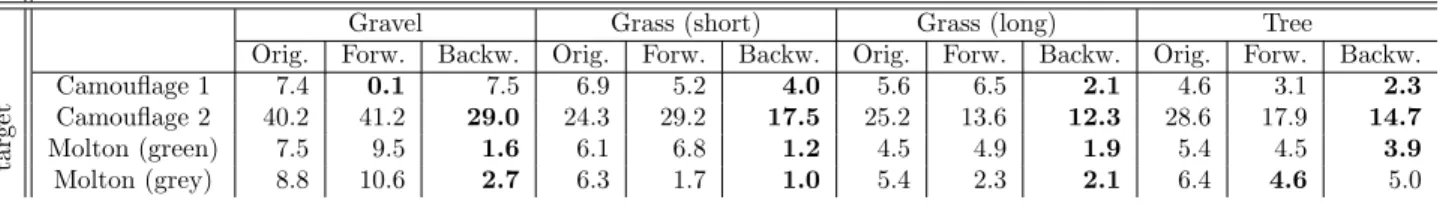
Table 2. Mean detection limit for aisaHawk data. Results are given as the mean minimal fraction of a pixel covered by the target at 0.1 % false alarm rate.
background
Gravel Grass (short) Grass (long) Tree
Orig. Forw. Backw. Orig. Forw. Backw. Orig. Forw. Backw. Orig. Forw. Backw.
Camouflage 1 7.4 0.1 7.5 6.9 5.2 4.0 5.6 6.5 2.1 4.6 3.1 2.3 tar ge t Camouflage 2 40.2 41.2 29.0 24.3 29.2 17.5 25.2 13.6 12.3 28.6 17.9 14.7 Molton (green) 7.5 9.5 1.6 6.1 6.8 1.2 4.5 4.9 1.9 5.4 4.5 3.9 Molton (grey) 8.8 10.6 2.7 6.3 1.7 1.0 5.4 2.3 2.1 6.4 4.6 5.0
ratios are chosen such that the amount of mixed spectra matches the number of lines of the data. Synthetic mixtures can then be appended to the image by continuing the data set with as many columns as the number of target pixels multiplied by the number of background pixels. Each simulated column ranges from 100 % target pixel and 0 % background at the bottom to 0 % target and 100 % background on the top. An example for the resulting synthetic VNIR data for the mixture ofMolton (gray) withGravel is depicted in Figure 2. As molton is homogeneous the mixtures look identical for higher target ratios but start to look different once the variation of the background comes into play.
Image statistics for the ACE classifier are calculated from the data without simulated mixtures and target areas. Black rectangles in Figure 2 signify former target areas. In a practical environment camouflaged targets are usually small enough to have a negligible effect on image statistics. When the statistics mirror the target spectrum, detection results are considerably lower.
To limit computational complexity spectral binning by a factor of 2 is performed on all data sets. Also, the number of spectral bandspin the final band selection data set is limited top= 20.
4. RESULTS
The results for detection limits are computed using two different band selection approaches from chapter 2. Evaluation in each iteration is performed by calculating the mean minimal target fraction in a given mixture. For this we set the acceptable false alarm rate to 0.1 % of image pixels. Together with all possible mixtures one target and background spectrum constitute one column of simulated data. During classification pixels with higher target ratios are detected before the ones with lower ratios. Thus, the mean of all minimal detected fractions for one target-background combination is a good indication of performance.
Results are computed for 4 target and 4 background materials and a desired number ofp= 20 remaining bands. Tables 1 & 2 show the results for each combination. Best results for each mixture are written in bold.
The mean spectrum of each target area is used as reference for ACE classification in each iteration of the bandselection procedure. The reference is adjusted to fit the bandselection in each step.
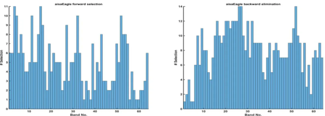
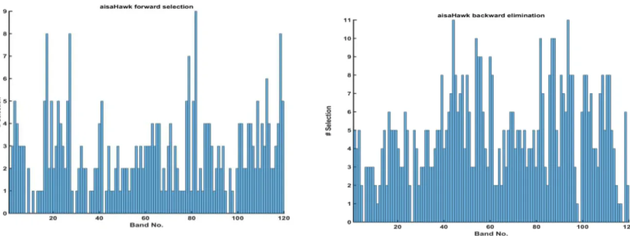
Figures 3 & 4 depict the histograms of band usage over all combinations for aisaEagle and aisaHawk data for both bandselection procedures.
5. DISCUSSION
A discussion of varying behavior of different mixtures in original data can be found in Gross et al.1
Especially the difference between Camouflage 1 and Camouflage 2 in SWIR data is prominent and can be explained by
aisaEagle forward selection
10 20 30 40 SO 60
Band No.
aisa Eag a backward elimination
10 30
Band No. different material composition.
The results from Tables 1 & 2 show that bandselection can improve the approximated detection limit when com-pared to the original results. Depending on the target and background spectra even small fractions of target can be enough for correct classification. TheBackwards Elimination with Internal Clustering is superior in almost all cases for aisa data. Forward Selection with Internal and External Clustering still has better results compared to classification on original data for most combinations of target and background spectra. A possible explanation could be different numbers of spectral bands used for the bandselection. While the remaining number of bands is alwaysp= 20, during backwards elimination many more bands are clustered and the bandselection results make use of wider wavelength ranges.
Analyzing results during iteration show steep decrease of minimal detected target size after 1–5 bands were selected. Beyond that approximated detection limit only gradually improves. DuringBackwards Elimination with Internal Clustering results gradually improve during clustering/elimination showing a maximum around 30 bands. After that, results decrease as the algorithm is forces to discard useful information eventually.
Computational complexity of both bandselection procedures can be improved by parallel implementation since classification and evaluation for each step of iteration is independent. CalculatingBackwards Elimination with Internal Clustering requires more time since each classification/evaluation step is done with a number of bands strictly greater thanp, whileForward Selection with Internal and External Clustering always operates with less thanpbands until it terminates.
Histogram plots of used bands for all combinations don’t hint at single bands but rather certain wavelength ranges that are important for robust classification. Histograms are depicted in Figure 3 for aisaEagle and Figure 4 for aisaHawk results. Values above 4 for a single band indicate it was selected for more than one target or background. Backwards Elimination with Internal Clustering exploits the clustering option much more often, usually resulting in 25–45 bands used for the resulting data set. In contrast,Forward Selection with Internal and External Clusteringusually has 20–23 bands, rarely clustering at all. Looking at Figure 4 gaps in the histogram don’t exactly match wavelengths of atmospheric absorption, indicating they still contain useful information. A discussion of specific cases where only narrow features exist could not be done with the available targets. One example would be the detection of oil spills as in Keskin et al.5
Figure 3. Histograms of commonly used bands for aisaEagle forward selection (left) and backward elimination (right) results for all combinations of target and background from Table 1.
6. OUTLOOK
The results show that a clever selection of bands or wavelength intervals can increase the chance of detection. One drawback is the computational complexity ofForward Selection with Internal and External Clustering and Backwards Elimination with Internal Clustering. Testing for all possible band combinations sequentially quickly becomes infeasible with increasing number of bands or bigger data sets. A possible approach is to calculate the
0
aisallawk forward selection
20 40 60 Band No 80 100 120 11 10 9 ] 0
aisaHawk backward elimination
20 40 60 80 100 120
Band No.
Figure 4. Histograms of commonly used bands for aisaHawk forward selection (left) and backward elimination (right) results for all combinations of target and background from Table 2.
best band combinations again for subsampled data or data with spectral binning. A comparison of the results can help to determine the ideal tradeoff between computational complexity and classification result.
Further, the computational time can be reduced by parallel implementation of each method. Since each selec-tion/elimination requires multiple independent classification and evaluation steps, this can be easily achieved. Using extracted target and background spectra the remaining analysis can be performed automatically. A trans-fer of these results to generalize statements of detection limits for other weather and illumination conditions is of interest. Suitable data is required to test if the same bands are selected for a specific target/background combination when the illumination or weather conditions change.
Since both bandselection algorithms are brute force approaches other methods should be tested to compare results. Promising approaches have been shown by Zhang et al.6
and Chang et al.7
Both methods try to deter-mine important features from the data. It remains to be seen if those procedures can actually be used for target detection, since automatic procedures usually model the data based on quantitative occurence of materials to minimize the approximation error. Specific target signatures could be truncated in the process since their impact on image statistics is negligible.
Also, other target and background combinations should be analyzed since the question about universally useful bands or wavelengths could not conclusively be answered.
Other methods to target and background simulation are proposed by Cohen8 and Guanter9 and can be tested
to determine the robustness of bandselection and approximated detection limits under other conditions.
ACKNOWLEDGMENTS
This research was supported by WTD 81 - Wehrtechnische Dienststelle f¨ur Informationstechnologie und Elek-tronik; Eidgen¨ossisches Departement f¨ur Verteidigung, Bev¨olkerungsschutz und Sport VBS armasuisse Wis-senschaft + Technologie; WTD 52 - Wehrtechnische Dienststelle f¨ur Schutz- und Sondertechnik. We thank our colleagues from Fraunhofer IOSB and University of Zurich and University of Be’er-Sheba who provided insight and expertise that greatly assisted the research.
REFERENCES
1. W. Gross, J. Boehler, H. Schilling, W. Middelmann, J. Weyermann, P. Wellig, R. Oechslin, and M. Kneubuehler, “Assessment of target detection limits in hyperspectral data,” Proc. SPIE, Target and Background Signatures, 96530J9653, 2015.
2. F. Kruse, A. Lefkoff, J. Boardman, K. Heidebrecht, A. Shapiro, P. Barloon, and A. Goetz, “The spectral image processing system (sips) - interactive visualization and analysis of imaging spectrometer data,”Remote Sensing of the Environment44, pp. 145–163, 1993.
3. X. Jin, S. Paswater, and H. Cline, “A comparative study of target detection algorithms for hyperspectral imagery,” inSPIE Algorithms and Technologies for Multispectral, Hyperspectral, and Ultraspectral Imagery XV,Proc. SPIE7334, pp. 1–12, 2009.
4. L. Yu, H. Liu, and I. Guyon, “Efficient feature selection via analysis of relevance and redundancy,”Journal of Machine Learning Research5, pp. 1205–1224, 2004.
5. G. Keskin, C. D. Teutsch, A. Lenz, and W. Middelmann, “Concept of an advanced hyperspectral remote sensing system for pipeline monitoring,” inEarth Resources and Environmental Remote Sensing/GIS Appli-cations VI, Proc. SPIE9644, pp. 96440H–96440H–9, 2015.
6. A. Zhang, G. Sun, and Z. Wang, “Optimized hyperspectral band selection using hybrid genetic algorithm and gravitational search algorithm,” inMIPPR 2015: Parallel Processing of Images and Optimization; and Medical Imaging Processing,Proc. SPIE9814, pp. 981403–981403–6, 2014.
7. Y.-L. Chang, J.-N. Liu, Y.-L. Chen, W.-Y. Chang, T.-J. Hsieh, and B. Huang, “Hyperspectral band selection based on parallel particle swarm optimization and impurity function band prioritization schemes,” Journal of Applied Remote Sensing8(1), p. 084798, 2014.
8. Y. Cohen, Y. August, D. G. Blumberg, and S. R. Rotman, “Evaluating subpixel target detection algorithms in hyperspectral imagery,”Journal of Electrical and Computer Engineering2012, p. 15, 2012.
9. L. Guanter, K. Segl, and H. Kaufmann, “Simulation of optical remote-sensing scenes with application to the enmap hyperspectral mission,”Geoscience and Remote Sensing, IEEE Transactions on 47, pp. 2340–2351, July 2009.