Novel Preprocessing Approaches for Omics
Data Types and Their Performance Evaluation
Dario Strbenac
A thesis submitted in fulfilment of the requirements for the degree of Doctor of Philosophy
School of Mathematics and Statistics
The University of Sydney
degree or for other purposes. All of the assistance received in preparing this thesis and sources have
Abstract
A diverse range of high-dimensional datasets has recently become available to help elucidate the functioning of biological systems and defects within those systems leading to disease. This improved understanding will aid our knowledge of fundamental biology as well as increasing our comprehension of the processes that are altered in complex disease. All of these new technologies come with the challenges of determining how the raw data should be efficiently processed or normalised and,
subsequently, how can the data best be summarised for more complex downstream analysis. There are many approaches to summarising and normalising omics data, with new methods frequently being developed. Different kinds of omics data may also be integrated, in order to provide more confidence in predictions. To date, there has not been a comprehensive evaluation of existing methods for many omics data types. This thesis focusses on systematically evaluating existing methods for three different types of omics data and, having identified limitations in the current methods, also proposes new approaches to improve their quality.
Firstly, CAGE-seq data are considered. This type of data has unique characteristics such that regional summarisation algorithms developed for similar experiments, such as ChIP-seq, are not directly applicable. Additionally, the raw data also contain artefactual measurements from confounding biological processes, and a comprehensive evaluation of region classification algorithms has not
previously been carried out. A two-stage method based on a novel region-finding algorithm followed by a classifier that integrates sequence patterns surrounding the identified regions is shown to possess superior performance to two existing methods. Similarly, a novel data summarisation approach to gene expression data, which integrates changes in location and scale into a unified metric, demonstrates benefits in two-class classification problems. The error rates are found to be competitive with existing methods, and the feature selection has higher stability and increased biological relevance. Finally, in the proteomics setting, there are many choices for how to summarise peptides to proteins, as well as issues relating to batch effects and whether internal controls are necessary. By developing a broad variety of performance metrics that assess bias or variance, and an accompanying web-based framework for reproducible research, novel recommendations about peptide to protein summaries and batch correction algorithms are made, and a surprising result regarding the necessity of internal standards is revealed. The development and evaluation of novel dataset preprocessing approaches and the comprehensive evaluation of existing methods for three data types demonstrates the importance of systematic
Publications and Presentations
Some of the research in this thesis has appeared in peer-reviewed journals or conferences. Publications
Dario Strbenac, Nicola Armstrong and Jean Yang. (2013) Detection and classification of peaks in 5' cap RNA sequencing data. BMC Genomics, Supplement 5, S9.
Dario Strbenac, Graham Mann, John Ormerod and Jean Y.H. Yang (2015) ClassifyR: an R package for performance assessment of classification with applications to transcriptomics. Bioinformatics,
31(11):1851-1853.
Dario Strbenac, Graham Mann, Jean Y.H. Yang and John Ormerod (2016) Differential distribution improves gene selection stability and has competitive classification performance for patient survival. Nucleic Acids Research, 44(13):e119.
Presentations
Detection and classification of peaks in 5' Cap RNA sequencing data. 12th International Conference on Bioinformatics. 21 September 2013. Taicang, China.
Detection and classification of peaks in 5' Cap RNA sequencing data. 57th Annual Meeting of the Australian Mathematical Society. 1 October 2013. Sydney, Australia.
ClassifyR: Classification Convenience with R. Sydney Bioinformatics Research Symposium. 7 November 2014. Sydney, Australia.
Gene Expression Analysis and Classification of RNA-Seq Data Using R and ClassifyR. BioInfoSummer. 9 December 2015. Sydney, Australia.
For: Summarisation and Classification for CAGE-seq Data
The research presented in Chapter 2 has previously been published in the journal BMC Genomics and I am the corresponding author for the article. The project was motivated by Dario’s previous employment at the Garvan Institute, where he briefly worked on CAGE-seq analysis. Dario developed much of the two-stage TSS region algorithm and implemented it and the associated case studies in R. Features for the classifier were suggested and agreed upon by all participants. Classifier design involved input from all three participants. All publicly used datasets for integration were obtained and processed by Dario. The first draft of the journal article was written by Dario and it subsequently had major contributions from all three participants. Some additional unpublished evaluations are presented in Sections 2.2.1.1 and 2.3.
Acknowledgements
In the academic context, I am thankful to my supervisors Professor Jean Yang and Dr. Nicola Armstrong for their inspiration and guidance on this long and challenging journey. They have always encouraged me to try more ideas when a proposed idea failed to meet expectations. Thanks also to Dr. John Ormerod for his guest supervision of the differential distribution project. His unique views of the problem helped to improve the work to a level which is of importance to a wide readership. The
motivation for the project was partially provided by Professor Graham Mann, who has contributed many biological insights to the research, which ensures its translational relevance. All supervisors also
provided detailed advice in regards to academic writing, which improved the clarity of the work and the associated results. Also, I would like to acknowledge the infrastructure provided by the Department of Mathematics and Statistics. Without the two large-memory, many-CPU servers available,
computationally-intensive tasks such as large cross-validation would not be completed in good time. Finally, thanks to Sarah-Jane Schramm and Shila Ghazanfar for each proofreading a chapter.
The collaborators at the Bioanalytical Mass Spectrometry Facility at University of New South Wales have been a crucial part of the proteomics normalisation project. To complete the experiment, they had to dispense 21 proteins into 56 different tubes at a different volume in each tube. Such a difficult experiment has not been attempted before, and their patience and diligence enabled us to have the ideal dataset for methodology performance evaluation. Thanks are also due to Professor Susan Wilson for providing top-up salary funding, enabling the research to be properly and reproducibly done.
In the social context, I would like to thank my parents Drago and Darinka for the many visits they made to Sydney and the frequent assistance with domestic duties they provided. Last, but not least, I thank Jasmine, my girlfriend, for her patience and positive thinking.
1 Introduction ... 1
1.1 Fundamentals of Molecular Biology ... 1
1.2 Overview of Measurement Technologies and Their Data Types ... 3
1.2.1 Microarrays ... 4
1.2.2 High-throughput Sequencing ... 4
1.2.3 Mass Spectrometry-based Proteomics ... 6
1.2.4 Biological Annotation of Omics Data ... 7
1.3 Omics Data Methods Evaluation Challenges ... 8
1.4 Thesis Outline ... 10
2 Summarisation and Classification for CAGE-seq Data ... 11
2.1 Background ... 12 2.1.1 ChIP-seq ... 13 2.1.2 DNAse-seq ... 14 2.1.3 RNA-seq ... 15 2.1.4 CAGE-seq ... 15 2.1.5 HTS Mapping... 19
2.2 Two-stage Preprocessing Algorithm ... 20
2.2.1 Region-Finding ... 20
2.2.2 Classification of Regions ... 22
2.3 Case Study: Prostate Cancer ... 28
2.4 Discussion and Conclusion ... 30
3 Differential Distribution for Binary Classification Problems... 33
3.1 Background ... 34
3.2 Feature Selection and Classification ... 38
3.3 Evaluation Metrics ... 44
3.4 Simulation Evaluation of DV and DD Varieties ... 45
3.5 Evaluation of DE, DV, and DD ... 51
3.6 ClassifyR Classification Evaluation Framework ... 59
3.7 Discussion and Conclusion ... 61
4 Performance of Proteomics Summarisation and Normalisation Methods... 64
4.1 Background ... 66
4.1.1 Mass Spectrometry-based Proteomics ... 66
4.2 Performance Metrics ... 76
4.3 Web-based Application ... 79
4.4 Case Studies ... 83
4.4.1 Case 1: Preprocessing with ProteinPilot ... 83
4.4.2 Case 2: Custom Relative Quantitation ... 85
4.4.3 Case 3: Absolute Quantitation ... 90
4.5 Discussion and Conclusion ... 93
5 Conclusion ... 97
A Supplementary Material For Chapter 2 ... 100
A.1 Region Finding Visual Evaluation ... 100
A.2 Feature Selection ... 101
A.3 Parameter Tuning ... 103
A.4 Classification Performance ... 104
A.5 Prostate Cancer Case Study ... 104
B Supplementary Material For Chapter 3 ... 106
B.1 ClassifyR Runtime ... 106
B.2 ClassifyR Parameters ... 107
B.3 Properties of Biological Datasets ... 109
B.4 Most Stable Feature ... 110
C Supplementary Material For Chapter 4 ... 112
C.1 Full Specification of Latin Squares Experimental Design ... 112
C.2 Exploratory Analysis of Latin Squares Dataset Characteristics ... 115
C.3 Parameter Selection For Methods Comparisons ... 118
C.4 Scaling Factor Unchanged Slope Proof ... 118
Figure 1.1 The Central Dogma of Molecular Biology. The DNA in a cell exists as a pair of strands of nucleotides that are bonded (vertical grey lines). The sequences of nucleotides contain instructions for making RNA molecules. Once the information is transcribed to RNA form, it is usually translated into a sequence of amino acids termed a protein, although it can be converted back into DNA. Adapted from Fu et al. (2014, p. 294). ... 2 Figure 1.2 The DNA double helix. Each strand has a 5’ and a 3’ end, giving the two strands
an antiparallel orientation. The two possible bonds are C to G and A to T Adapted from Becker et al. (2008, p.59). ... 2 Figure 1.3 Two Ways to Measure DNA and RNA. For RNA experiments, the molecules are
firstly converted into DNA. Amplification of DNA is necessary to create an adequate number of measurable molecules. The molecules have to be broken into shorter fragments to allow them to be measured. Microarrays use fluorescent labelling of fragmented molecules and their binding to probes arrayed on a glass surface. HTS determines the sequence of the fragmented molecules. The count of sequences originating from a genomic region is proportional to its cellular abundance. This figure is hand-drawn. ... 6 Figure 2.1 Basic steps of histone ChIP-seq. The black line is part of a chromosome. The
grey cylinders are histones. The green circle represents a histone modification of interest. Firstly, the DNA is fragmented, and then only the histones that have the modification of interest are purified. The histones are then removed so that only the DNA remains and its sequence is determined. Adapted from Park (2009, p. 671). .. 14
Figure 2.2 Basic steps of DNAse-seq. The black line is part of a chromosome. The scissors are representative of DNAse I. The enzyme cuts in location that are not bound to protein, represented by orange and grey shapes. The resulting DNA fragments are sequenced to determine regions of unbound DNA. Adapted from Zentner and
Henikoff (2014, p. 816). ... 15 Figure 2.3 Key steps in the workflow for analysing CAGE-seq data. The cDNA sequences
obtained from the sequencer (Step 1) are aligned to the reference genome (Step 2). Only the first position of each read is retained, and the retained positions are
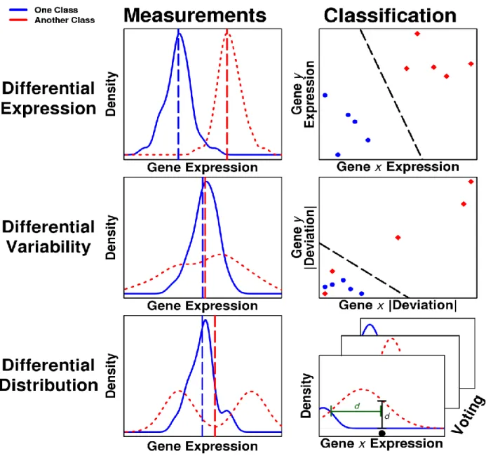
clustered into regions (Step 3). Lastly, a classification algorithm is used to label the regions as being from transcription initiation or not (Step 4). The focus of this study is on steps 3 and 4. ... 16 Figure 3.1 Summary of feature types and classifiers. For each of differential expression,
differential variability, and differential distribution, a representative gene expression distribution is shown, along with an illustration of the classification process. In the left column, the dashed vertical lines represent the means of the class distributions. In the right column, the variables 𝑥 and 𝑦 denote two different genes in a dataset. Each point indicates a sample. The bottom right panel illustrates that each gene from the selected gene set votes independently in differential distribution classification. The black circle shows the position along the x-axis of the expression measurement value. The intervals show two kinds of distance weighting evaluated in the simulation study. The green interval corresponds to crossover distance voting and the black interval to height difference voting. ... 42
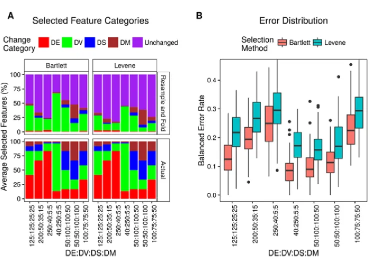
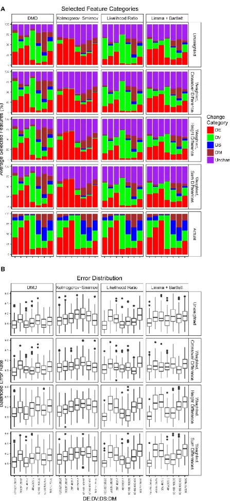
seven simulated datasets.A. Proportions of selected genes. The average
percentage of selected genes that are in the specified simulated change categories over all cross-validations is shown. The bottom row shows the proportions of
simulated changes. B. Balanced error rates of class predictions. The distributions of error rates across all cross-validation iterations are shown as boxplots. ... 48 Figure 3.3 Feature selection proportions and balanced error rates of DD classification
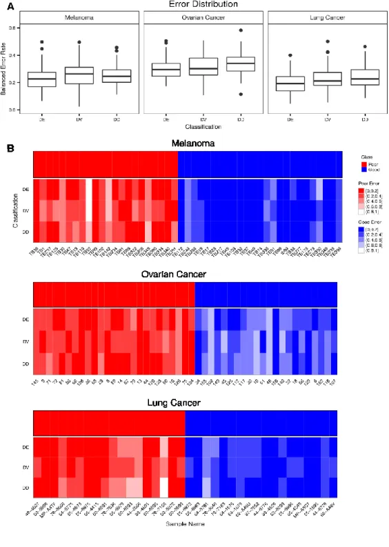
for seven simulated datasets.A. Proportions of selected genes. The average percentage of selected genes that are in the specified simulated change categories over all cross-validations is shown. The fifth row shows the proportions of simulated changes. B. Balanced error rates of class predictions. The distributions of error rates across all cross-validation iterations are shown as boxplots. ... 50 Figure 3.4 Cross-validation balanced error rates and sample-wise error rates.A.
Distribution of balanced error rates over all iterations of cross-validation. B. Sample-wise error rates. Each patient is one column of a heatmap. Each classification type is one row of a heatmap. Details of the selection and classifier algorithms are provided in the Methods section. The error rates are binned into five equally sized bins. Colour scales are shaded by class colour, with a darker colour indicating less frequent misclassification than a lighter colour. ... 54 Figure 3.5 Feature ranking and selection overlaps.A. Overlaps between three feature
selection types for three cancer datasets. The 50 highest-ranked genes of each method are used. All samples are used. B. Overlaps between three feature selection approaches for three cancer datasets. The genes selected by best resubstitution
error rate of each method are used. All samples are used. C. Cumulative MalaCards scores for the most frequently selected features in cross-validation. ... 56 Figure 3.6 Cross-validation feature ranking and selection stability. For each pair of
comparisons, the number of genes in common is divided by the number of genes in the union and converted to a percentage. A. The average pairwise overlap of the top ranked genes is calculated for all iterations of cross-validation. Shapes represent datasets and colours represent different types of classification. B. The distribution of the pairwise overlaps of the selected genes is calculated for all iterations of cross-validation. From left to right, the number of data points which are greater than 20% and are not shown as points is: 475, 16879, 5301, 305, 593, 5884, 963, 2489, and 29384. ... 58 Figure 4.1 Flowchart of proteomics data preprocessing. Steps of preprocessing are
represented by boxes and particular methods to evaluate are listed on the right side. Grey steps or option lists are not evaluated in this study. ... 69 Figure 4.2 Overview of the web-based application for evaluation.A. The New Processing
Upload page allows users to describe various aspects of their data preprocessing and to upload the protein quantities or fold changes as a text file to the server. The web-based application calculates all of the performance metrics and then
automatically switches to the Evaluation Matrix page. B. The Evaluation Matrix page displays the matrix of performance metrics and various tools to interact with it. The numbers in the table are summaries, either the mean or standard deviation of the metric, of either all experimental runs or all iTRAQ channels, where applicable. Filtering, sorting, row and column selection are used to subset the matrix to the
the column number. Numerical and graphical evaluation tools are located below the metric matrix. ... 82 Figure 4.3 Performance metrics of regression for relative quantitation using the default
processing parameters of ProteinPilot 5. Horizontal red line represents the ideal metric value. Metrics are grouped either by iTRAQ channel (first row) or run (second row). ... 85 Figure 4.4 Performance metrics for relative quantitation. Horizontal red line represents the
ideal metric value. ... 90 Figure 4.5 Performance metrics for absolute quantitation. Horizontal red line represents
the ideal metric value. A. The distribution of metric values of a linear regression of protein summaries within a sample divided by the median protein group’s median summary of the sample, grouped either by iTRAQ channel or experimental run. B.
Summaries for three variance metrics calculated using data from either one run or all runs. ... 92 Figure A-1 Raw counts and detected regions for sample GM12878. The first two rows show
the counts at each position of the first positions of CAGE reads. The Genes row shows a model of known genes in this region. The left-most edge of the blue rectangle is a known TSS. The thin blue lines are known introns. The bottom three rows show the regions determined by each of the three methods compared. The angle brackets show the strand on which the regions are. “>” represents the plus strand and “<” represents the minus strand. ……...101
Figure A-2 Principal components analysis of the scalar features surrounding the CAGE read regions. The top panel shows the TSS category of regions and the bottom panel shows those regions which are labelled as Not TSS in the truth set. Dots represent the 100 observations in the lowest density regions. ……….……102 Figure A-3 Principal components analysis of the 4-mers surrounding the CAGE read
regions. The analysis was performed on the correlation matrix of the 512 4-mers. The top panel shows the TSS category of regions and the bottom panel shows those regions which are labelled as Not TSS in the truth set. Dots represent the 100 observations in the lowest density regions. ……….103 Figure A-4. Precision and recall for three feature scenarios. Precision and recall are
calculated at each cost parameter value based on a LOOCV scheme. Blue lines are precision. Red lines are recall. Horizontal bars or dots represent the minimum and maximum value of all cell lines. Points on the line are averages across all six cell lines for the two leftmost panels and two cell lines for the rightmost panel. 104 Figure A-5. CAGE count summaries for the genes with the best differential expression
and TSS switching statistics. The top two rows of data show normalised count values per genomic position in each of the two experimental conditions. The third row of data shows the structure of known genes. The bottom row shows the regions which have been classified as TSS regions. ……….…………..……106 Figure B-1 Distribution of survival times for the three cancer datasets used for
classification evaluation. Densities are estimated with the default Gaussian kernel in R. ………111
three datasets and three feature types. The RefSeq symbol of the gene the densities are plotted for is shown above each density plot. DV selection is made by ranking of the Bartlett’s test statistic and DD selection is made by the proposed DMD statistic. ………..…………112 Figure C-1 Relationship between length of spike-in protein and number of peptides
detected in experiment. The number of peptides associated to a spike-in protein based on matching by ProteinPilot’s Paragon algorithm is shown for all seven runs. ………...……117 Figure C-2 Principal components analysis of background proteins. Seven yeast proteins
were quantified in all seven runs. For each sample, the dimensionality has been reduced to two dimensions. Each row of plots contains yeast protein
measurements summarised from peptides in one of the three summary methods used in this study. The first column has samples coloured by experimental run and the second column has samples coloured by iTRAQ channel. ……….…….118
List of Tables
Table 2.1 Number of regions detected for each cell line. The proposed sliding window, Paraclu and F-seq are evaluated. ... 21 Table 2.2 Percentage overlap between proposed method’s regions and those found by
Paraclu and F-seq. Regions must have at least one base overlap and be on the same genomic strand to be considered as overlapping. ... 22 Table 2.3 Features considered for TSS classification. For each feature, the summarisation
procedure, location of data points summarised, and the feature categorisation are shown. ... 25 Table 2.3 Precision and recall values for the internal features LOOCV classification. For
each cell line, classifier training was performed on the five other cell lines. A cost parameter of 0.1 is used for the linear SVM classifier. ... 28 Table 4.1 Experimental Design for Run 1. The values in the table are volumes of diluted
protein used, in units of microlitres. ... 75 Table 4.2 Summary of performance metrics and their characteristics. The applicability of a
metric to the quantitation type, preprocessing stage, and error characteristic is shown. (R): only affects relative quantitation. The number next to the metric name shows its column name in the web-based application. ... 79 Table A-1 Precision and recall for three dataset scenarios. Internal scenario uses selected
4-mers. Internal and Pooled External scenario uses selected 4-mers and Maximum H3K4me3, Maximum TFBS, Maximum Sensitivity, and Average Conservation
test of flanking RNA-seq counts, matched to each cell line. Grey cells indicate
evaluations for which data is not available. ...…105 Table B-1 Classification runtime using ClassifyR. DE and DV classification were evaluated
in two cross-validation modes, using between 1 and 16 processing cores. ….…..108 Table B-2 Parameter classes and their required variables. Classes that store parameters
for each stage of classification and the meanings of each parameter. Any other variables can be stored and used, as long as the function which performs the particular stage knows how to use them. In addition, all classes use a parameter
intermediate, which is a character vector of variable names generated internally by runTest that will be used in the classification stage the class
represents. ………..………109 Table C-1 The identities of purchased proteins and their associated information. Group
denotes the allocated group label of each protein, so that a variety of sizes are in each group. ……….113 Table C-2 Experimental design of all seven runs for the purchased proteins. The volumes are in units of microlitres. ………..114 Table C-3 Percentage of peptides in a particular run detected in another run. The
percentage of peptides in each run that overlap with each other run is displayed. ………116 Table C-4. Number of proteins identified in each run. The number before the slash is for
protein identification by at least one peptide. The number after the slash is the number of proteins with at least three matched peptides. ………...117
Table C-5 Performance metrics after normalisation of Top 3 peptide summaries of proteins. The best value for a parameter combination is highlighted as a white metric value with a black background, if the difference between the lowest and highest value is at least 25% of the highest value. A For Simple Scaling and Two-stage Scaling considering four representations of the yeast proteins. B For RUV. k
is the rank parameter and ν is the regularisation parameter. Number shown in a cell is the mean of metrics, where there is more than one metric calculated. …121
Abbreviations
BER Balanced Error Rate
CAGE Capped Analysis of Gene Expression ChIP Chromatin Immunoprecipitation
CV Coefficient of Variation
DNA Deoxyribonucleic Acid
KDE Kernel Density Estimate
HMM Hidden Markov Model
HTS High-throughput Sequencing
IQR Interquartile Range
iTRAQ Isobaric Tags for Relative and Absolute Quantitation LOOCV Leave-One-Out Cross-validation
MS Mass Spectrometry
µL Microlitre
PCA Principal Components Analysis
RNA Ribonucleic Acid
RUV Removing Unwanted Variation
SVM Support Vector Machine
TFBS Transcription Factor Binding Site TSS Transcription Start Site
1
Introduction
Major advancements to the understanding of living systems and complex diseases enabled by new developments in biotechnology and statistical bioinformatics are beginning to transform modern life. The developments in biotechnology often provide indirect measurements of the biological entities of interest and have particular types of noise or bias; problems which are essential to consider for
knowledge discovery. The associated development of new statistical methods and their evaluation in this and other contexts has the potential to deliver improved biological understanding and advance medicine. A basic introduction to the biology and biotechnology required for this thesis follows. Firstly, the key biological molecules that are measured and their purpose is described. Next, the technologies which are used to obtain the identities and quantities of the biological molecules are introduced. Thirdly, some challenges with evaluating statistical methods for omics data processing are highlighted. Readers familiar with molecular biology and the omics measurement technologies are recommended to skip to Section 1.3.
1.1 Fundamentals of Molecular Biology
Life is the continual flow of information from molecules to other types of molecules, to accomplish tasks such as cell growth, metabolism, and defence from disease. The major information pathway in all living cells is the encoding of information from deoxyribonucleic acid (DNA) sequences to ribonucleic acid (RNA) sequences to protein sequences and was first described over fifty years ago (Crick, 1958). The processing of DNA into RNA is termed transcription and the processing of RNA into protein is
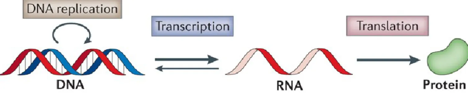
referred to as translation. The theory left room for information to flow in the reverse direction from RNA to DNA, as shown in Figure 1.1, which was experimentally confirmed twelve years later by two research groups (Baltimore, 1970; Temin & Mizutani, 1970).
Figure 1.1 The Central Dogma of Molecular Biology. The DNA in a cell exists as a pair of strands of nucleotides that are bonded (vertical grey lines). The sequences of nucleotides contain instructions for making RNA molecules. Once the information is transcribed to RNA form, it is usually translated into a sequence of amino acids termed a protein, although it can be converted back into DNA. Adapted from Fu et al. (2014, p. 294).
The three categories of biological molecules are comprised of different fundamental units and have vastly different structures, which is why the technologies used to identify and measure them are largely different.
DNA: The genome contains much of the information necessary for an organism to develop and live. The fundamental information units of DNA are the four bases: adenine (A), guanine (G), cytosine (C) and thymine (T). Two strands of DNA are bound to each other with only bonds between A and T, and G and C being possible (Figure 1.2). Each strand has a particular modification at its ends and the 3’ or 5’ notation denotes the position of the modification on the sugar
Figure 1.2 The DNA double helix.
Each strand has a 5’ and a 3’ end, giving the two strands an antiparallel orientation. The two possible bonds are C to G and A to T Adapted from Becker et al. (2008, p.59).
1.2 Overview of Measurement Technologies and Their Data Types ring. The segments of the DNA sequence which contain instructions for making RNA sequences are called genes.
RNA: Unlike DNA, which is the same in every cell of an organism, the collection of RNA sequences present, called transcripts, and their abundances are different between cells and change over time. The first base of synthesised RNA is said to be the 5’ end of the molecule and the last base is the 3’ end. The first base is also referred to as the transcription start site, or TSS. It has a particular cap structure on it. The template strand is the strand of DNA read by the RNA polymerase. Sequences towards the 3’ end of the coding strand of the DNA are said to be downstream of the TSS, whereas sequences towards the 5’ end are said to be upstream. The region upstream of the TSS which has a regulatory function is termed the promoter. Segments of the newly created RNA molecule which are excised are called introns. The contiguous genomic regions of the sequence that remains after the introns are removed are called exons. Proteins: The functional entities which perform most of the tasks in a cell. Each cell is capable of expressing thousands of different proteins. All the proteins in an organism are referred to as the
proteome (James, 1997). To translate a RNA sequence into a protein, the sequence is parsed in groups of
three bases, always starting at AUG and ending at one of three base combinations. Parsing always occurs from the 5’ end towards the 3’ end of the RNA molecule.
1.2 Overview of Measurement Technologies and Their Data Types
The three types of biological molecules considered here (DNA, RNA and proteins) are comprised of different fundamental units and have vastly different structures. Hence, a range of experimental methods have been developed to measure and characterize different aspects of this system and in turn, a variety of complex data structures have been generated. Understanding and efficient processing of such
complex and high-dimensional data sets poses a range of challenges for modern statistics, including those of normalisation and summarisation.
In this thesis, the biotechnology platforms considered are microarrays and high-throughput sequencing (Chapters 2 and 3), and mass spectrometry (Chapter 4). These platforms, and the type of data generated, are described in detail below.
1.2.1 Microarrays
Microarrays are a grid of regularly-spaced probes. Each probe has a particular sequence of nucleotides that matches to a certain genomic location; this sequence is chosen to be unique to one location in the genome. The molecules are first amplified and then labelled with a chemical that fluoresces. The abundance of each probe can be determined by the intensity of the fluorescence at a particular place in the grid. Each probe represents a genomic region that surrounds the probe, whose boundaries are determined by the lengths of the nucleic acid molecule fragments created during sample preparation. The value is a continuous measurement. Molecules which have some mismatches to the probe sequence can also bind to the probe, meaning that some probes undesirably measure a combination of different genomic locations (Koltai & Weingarten-Baror, 2008). This is termed cross-hybridisation. Another drawback is that genes which have no associated probes on the microarray, but are discovered after the manufacture of the microarray, are unable to be measured unless the experiment is repeated with a newer model of microarray. Two of the datasets used for differential distribution evaluation are microarray datasets (Chapter 3).
1.2.2 High-throughput Sequencing
In contrast to microarrays where the probes are predefined by design, high-throughput sequencing (HTS) determines the nucleotide sequence of tens of millions of DNA or RNA fragments, often simply
1.2 Overview of Measurement Technologies and Their Data Types referred to as reads. Using a predefined database of regions of interest and counting the number of reads mapped within them allows estimates of abundances to be calculated. HTS has some important
advantages over microarrays (Wang, Gerstein, & Snyder, 2009). Firstly, it can allow the discovery of new genomic features that are not yet found in genome databases. Secondly, microarrays have both background fluorescence and can reach saturation if the number of molecules of a certain sequence is greater than the number of probes of that sequence. For HTS, there is no background signal, and saturation is also not an issue. Lastly, as explained in the previous section, cross-hybridisation is a problem of probe-based technology, which HTS is not. One disadvantage of HTS is that it is based on simple random sampling of fragments, which means that some lower abundance molecules may not be sequenced, depending on the abundance of the most common molecules. Secondly, fragments must be associated with biological features of interest, such as genes or proteins. A summary of the two
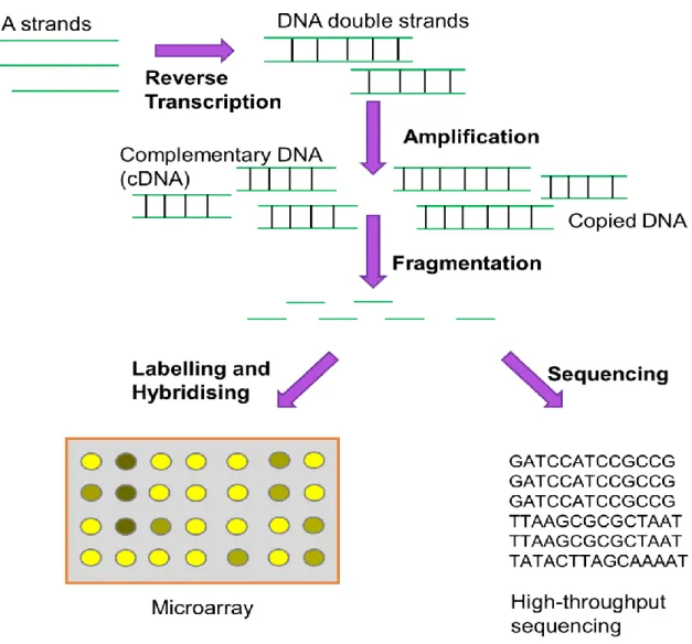
technologies is shown in Figure 1.3. HTS datasets form the basis of CAGE-seq data analysis and dataset integration (Chapter 2) and one of the datasets that is utilised for evaluation of differential distribution (Section 3.5).
Figure 1.3 Two Ways to Measure DNA and RNA. For RNA experiments, the molecules are firstly converted into DNA. Amplification of DNA is necessary to create an adequate number of measurable molecules. The molecules have to be broken into shorter fragments to allow them to be measured. Microarrays use fluorescent labelling of fragmented molecules and their binding to probes arrayed on a glass surface. HTS determines the sequence of the fragmented molecules. The count of sequences originating from a genomic region is proportional to its cellular abundance. This figure is hand-drawn.
1.2.3 Mass Spectrometry-based Proteomics
Unlike the simpler structures of DNA and RNA, proteins have more complicated 3D forms, and their identification and quantitation are more difficult. RNA and protein levels are sometimes not highly
1.2 Overview of Measurement Technologies and Their Data Types correlated (Gry et al., 2009), because of various regulatory mechanisms that affect the rates of
translation and protein degradation. Therefore, it is desirable to be able to accurately identify proteins and measure their abundances. Mass spectrometry (MS) is the most popular technique for these tasks. It is based on propelling protein fragments through a magnetic field in a vacuum, which separates
fragments based on their sizes (Weickhardt, Moritz, & Grotemeyer, 1996). The size of the signal created by protein fragments hitting the detector is proportional to the number of those fragments in the sample. A more detailed background is given in Section 4.1.1.
1.2.4 Biological Annotation of Omics Data
Microarrays, HTS, and MS interrogate a large number of molecular sequences. By design, all
microarray probes are annotated to known biological features. To give biological meaning to HTS- and MS-derived sequences, it is necessary to match the sequences to known genes or proteins. There are large databases of experimentally characterised genes and proteins for well-studied organisms, such as human or mouse. For example, RefSeq and UniProt are two such databases (NCBI
Resource Coordinators, 2015). Many of the genes and proteins in these databases have known functions, which enables biologists to suggest which cellular mechanisms might be important to their topic of study. The computational matching is largely different for HTS and MS data. A more detailed background is provided in Section 2.1.5 for HTS data and Section 4.1 for MS data.
A common challenge that is shared by various bioinformatic methods for mapping high-throughput data is that they need to be tolerant of minor differences between the experimental sequences and the
database sequences. These can occur because the instrument makes an error determining the molecule’s sequence or because the sample under study has a genuine difference to the one found in the database, potentially related to the condition under study. Another challenge is the level of flexibility in handling ambiguity. The short sequences may match multiple locations in the genome, or multiple proteins in the
protein database. The software implementations of these mapping algorithms provide user-specified options to whether such sequences are reported, which affects summarisation of the raw data and its subsequent statistical analysis. Such ambiguities may bias the measurements, if ignored.
1.3 Omics Data Methods Evaluation Challenges
The widespread availability of complex biological data has necessitated a corresponding advancement in statistical methods. There exists a plethora of algorithms and methods that address issues from pre-processing tasks, such as data summarisation and normalisation, to more complex analyses, such as finding enriched networks of genes in a particular condition. The issue of finding an unbiased and meaningful way to accurately evaluate existing and newly proposed methods remains challenging. Also, accuracy and precision in many settings are suboptimal and may be improved with new approaches. Below, three issues that are related to the challenges explored in this thesis are described.
Absence of a Truth Set for Performance Comparison
For a particular biotechnology, many choices of data summary and normalisation methods are available. Some methods have been adapted from other types of datasets, while others have been developed with the specific technology in mind. For example, the boundaries of signal regions derived from sequencing data are difficult to evaluate, because no database contains a comprehensive set of regions and, indeed, the regions may differ by biological condition. This has resulted in efforts where domain experts have been tasked with manually viewing a small subset of the data and creating a database of regions based on their expert judgement (Hocking, Rigaill, & Bourque, 2015). The regions selected were found to be highly consistent between researchers. Other region-finding evaluations have compared the DNA sequence within the regions to known binding patterns (Wilbanks & Facciotti, 2010). Unfortunately, these kinds of methods are only applicable to proteins where information on binding patterns is readily
1.3 Omics Data Methods Evaluation Challenges available and make no assessment about the suitability of the region boundaries. Thus, there is no
comprehensive method for region evaluation available; only reasonable approximations. Generalisability of Findings
For binary classification problems, cross-validation is a common technique used for performance assessment. By always using different samples to train models and to make predictions with, this identifies which of the fitted models are stable. Feature selection stability and prediction error rate distribution are two types of metrics which have previously been assessed by 10-fold cross-validation for two classes of breast cancer (Cun & Fröhlich, 2012). Apart from selection frequency, the overlap of the most frequently selected features and those in known gene pathways (Mann et al., 2013), is an alternative evaluation of feature selection. However, this approach may understate the importance of genes belonging to pathways not yet characterised in public databases. Cross-validation has been shown to have low stability for datasets with weak signals (Martinez, Carroll, Müller, Sampson, & Chatterjee, 2011), which motivates the use of dataset resampling with replacement together with cross-validation (Chapter 3). This approach gives a truer impression of classifier performance, rather than a point
estimate. A drawback of cross-validation is that it produces better performance metrics than training and predicting on independent datasets (Bernau et al., 2014), a process described as cross-study validation. In contrast, another evaluation study found a number of examples where the error rates of traditional cross-validation are equivalent or better than in cross-study validation (Schramm, Campain, Scolyer, Yang, & Mann, 2012), suggesting that cross-validation does give realistic representations of classifier performance.
Optimal Design of Experiments
Evaluation of preprocessing is simpler than the above two biologically-driven scenarios and is ideally performed with designed datasets, such as from a dilution series or spike-in design experiment. A dilution series design involves creating a complex mixture of the molecules under study, followed by manual dilution of the starting mixture to create samples with certain chosen ratios of change. The main difference between spike-in designs and dilution series is that a spike-in experiment is constructed with the same complex background mixture for every sample, but a small variety of molecules are added at particular amounts to each sample. Both types of studies allow the assessment of bias and variance. However, the absolute amounts of individual molecules cannot be controlled in dilution studies, limiting the number of possible comparisons. A spike-in study where each amount is present at every
combination of two factor levels is a Latin square design (Ryan, 2007) and is utilised in Chapter 4. A Latin square design allows two sources of unwanted variation to be accounted for with the minimum number of samples.
1.4 Thesis Outline
The remainder of this thesis is organised as follows. Chapter 2 presents a novel two-stage approach for CAGE-seq region-finding and classification, followed by a case study showing its ability to find existing and unknown changes of potential medical importance in a prostate cancer dataset. Chapter 3 proposes a new summarisation approach for gene expression data with performance improvements to existing methods and introduces a publicly available software implementation, ClassifyR. Then, in Chapter 4, a set of performance metrics to characterise bias and variance are created and a range of summarisation and normalisation approaches are evaluated by a newly developed web-based application which allows users to reproduce the research findings presented and also evaluate their own methods. Finally, the key contributions of this research are summarised in Chapter 5.
2
Summarisation and
Classification for CAGE-seq
Data
The introduction of HTS technologies provides new opportunities to characterise the mechanisms of disease. A broad range of applications have been developed, such sequencing of DNA to find mutations and copy number changes, enrichment of modified DNA and its sequencing to identify epigenetic deregulation, and sequencing of RNA to determine the functional regions of the genome. Capped Analysis of Gene Expression by sequencing (CAGE-seq) shows the diversity of transcription initiation across entire genomes. The identification of new transcription start sites will enable the discovery of new genes without any prior information and additionally may allow potential mechanisms of disease and development to be proposed. Two main challenges must be addressed to permit these discoveries. Firstly, transcripts do not precisely start in a single genomic position, but are distributed across a region. This creates the need for a fast and simple method of identifying transcription start regions. Secondly, due to biological processes other than transcription which also add 5’ caps to RNA molecules, many of the regions observed are not actually transcription initiation events. Classification of the
bioinformatically identified regions is an essential filtering step in the discovery of genuine
transcriptional initiation. The first independent evaluation of the only existing method designed for this task is presented, as well as another method based on integration of complementary datasets. Finally, a new method is developed that results in an improvement of classification performance.
In this chapter, a two-stage approach is described to identify the regions of true transcription initiation. Firstly, regions of enriched signal are identified by a fast and simple algorithm using a sliding window for counting read start positions and comparing to an empirical null distribution for declaring enriched regions. Secondly, a linear support vector machine classifier (Cortes & Vapnik, 1995), herein
abbreviated as SVM, is utilised to distinguish between regions that represent the initiation of transcription and regions that do not. Evaluation of classification performance shows significantly improved recall and similar precision to the two existing methods. Integration of external features derived from different cell lines to those with CAGE-seq data had similar precision and recall rates to using only features derived from CAGE-seq data. The addition of matched RNA sequencing data resulted in minor gains in recall while maintaining a similar level of precision.
The remainder of this chapter is organised as follows. Section 2.1 introduces CAGE-seq data and highlights the value of its analysis. Section 2.2 describes the new region-finding algorithm and makes comparisons to F-seq and Paraclu. It also explores the performance of the proposed region classifier and two competing methods. Having established the superior performance of the proposed region classifier, Section 2.3 demonstrates its use on a biological dataset of interest to determine changes in TSS regions between normal cells and prostate cancer cells.
2.1 Background
The locations of transcription start sites (TSSs) in the genome are of biological importance. There is rarely only a single TSS for a particular transcript (Frith et al., 2008), motivating their exhaustive enumeration. Clusters of TSS positions for a single transcript are referred to as TSS regions and
frequently occur in close proximity to transcription factor binding sites (TFBS). For example, the Prkd2 promoter contains a Gabp binding site (Yang et al., 2013). TFBS are known to regulate the packing of nucleosomes (Cairns, 2009), which determines the accessibility of the TSS region to the process of
2.1 Background transcription. When there is a loss of Gabp, Prkd2 expression is much reduced, and can lead to the development of chronic myelogenous leukaemia. Knowing the locations of the TSS regions reduces the genomic regions in which to search for regulatory motifs and generate hypotheses about the cause of changes in gene expression. Correct usage of alternative TSSs is also important for healthy development of the nervous system (Pruunsild, Kazantseva1, Aid, Palm, & Timmusk, 2007). This highlights the importance of transcription start detection to health and development.
Biological features which have been previously associated with TSS regions provide motivation for their genome-wide measurement by techniques such as ChIP-seq and DNAse-seq. Also, RNA levels
measured by RNA-seq can be informative for transcription initiation. First, a brief introduction to each experimental data type is given. Next, some important features of HTS mapping algorithms are
discussed. Finally, a detailed introduction to the focus of this chapter - CAGE-seq - is provided.
2.1.1 ChIP-seq
For gene transcription to be initiated or paused, certain proteins - called transcription factors - can bind to DNA and be detached from it. Also, histones, which are proteins that are attached to DNA, can be modified by other enzymes attaching or removing small molecules to them. The presence or absence of these proteins or their modifications can allow genes to be transcribed or prevent transcription from occurring (Park, 2009). For instance, a modification that is commonly known as H3K4me3 has been associated with transcription start sites undergoing transcription (Barski et al., 2007).
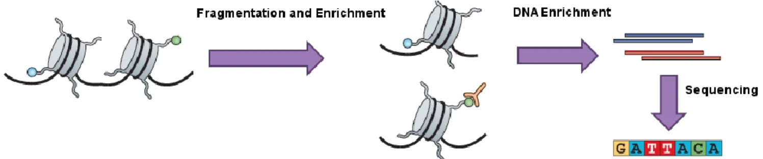
A ChIP-seq experiment designed for detecting a histone modification of interest is used for illustration. The experiment begins by fragmenting the chromosomes into smaller segments, followed by enrichment for the modification of interest (Figure 2.1). The complexes that have been enriched for are then
separated to keep only the DNA. Finally, the DNA is sequenced, which allows the characterisation of the regulatory functions of the modification.
Figure 2.1 Basic steps of histone ChIP-seq. The black line is part of a chromosome. The grey cylinders are histones. The green circle represents a histone modification of interest. Firstly, the DNA is fragmented, and then only the histones that have the modification of interest are purified. The histones are then removed so that only the DNA remains and its sequence is determined. Adapted from Park (2009, p. 671).
2.1.2 DNAse-seq
Like histone modifications and transcription factors, unwound DNA has also been associated with TSSs that are being transcribed (Sabo et al., 2006) and can be measured using DNAse-seq. Firstly, the DNA is exposed to the DNAse I enzyme. The enzyme cuts the locations of unbound DNA sequence into small fragments, while being unable to cut sections of DNA sequence obscured by proteins (Figure 2.2). Only the 5’ end of the sequenced fragment is used to build up a picture of where the cutting of DNA is taking place.
2.1 Background
Figure 2.2 Basic steps of DNAse-seq. The black line is part of a chromosome. The scissors are representative of DNAse I. The enzyme cuts in location that are not bound to protein, represented by orange and grey shapes. The resulting DNA fragments are sequenced to determine regions of unbound DNA. Adapted from Zentner and Henikoff (2014, p. 816).
2.1.3 RNA-seq
RNA-seq data can also provide supporting evidence for TSS regions, because transcription of a
particular gene only occurs in one direction along a chromosome. Therefore, it is expected that there are significantly more sequenced fragments on one side of the TSS region than the other. RNA-seq typically does not directly sequence RNA molecules, but their experimentally converted DNA representations, termed cDNA.
2.1.4 CAGE-seq
CAGE-seq can answer a number of biological questions of interest. Firstly, the analysis of its data allows the identification of the locations in the genome where the transcription of RNA molecules is initiated. This enables the discovery of new genes. Secondly, when samples from different biological conditions are available, tests for differential expression can be done. Genes may also undergo TSS switching. TSS switching describes the process where the starting location of a transcribed gene changes, irrespective of any changes in the transcript’s abundance. Changing the locations of the TSS usually alters which exons are present in the transcript, which results in a different protein product being made (Boley et al., 2014). The first nucleotide of a transcribed RNA molecule has a five-prime cap (5’ cap) attached to it. RNA molecules with a 5’ cap are extracted from cells and converted into DNA for
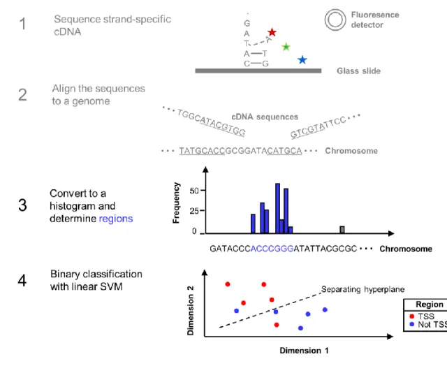
sequencing, which is the first step of the experiment. Once the reads are aligned to a genome, in the second analysis step, only the location of the first base is considered in further analysis. The third step involves finding regions of signal enrichment. Finally, in the fourth step, these regions must be classified as TSS regions or otherwise. The entire experimental process is summarised by Figure 2.3. CAGE-seq is inapplicable to some biological investigations, such as mitochondrial genes, which lack the 5’ cap (Grohmann, Amalric, Crews, & Attardi, 1978), and bacterial genes, which have a different cap modification to animals (Cahová, Winz, Höfer, Nübel, & Jäschke, 2015).
Figure 2.3 Key steps in the workflow for analysing CAGE-seq data. The cDNA sequences obtained from the sequencer (Step 1) are aligned to the reference genome (Step 2). Only the first position of each read is retained, and the retained positions are clustered into regions (Step 3). Lastly, a classification algorithm is used to label the regions as being from
2.1 Background CAGE-seq signal regions may be broad or narrow and they only appear on one strand, unlike ChIP-seq, so the development of specific region-finding methods to this datatype is necessary. Also, a caveat of CAGE-seq is that it detects all 5’ RNA caps, even those not related to the transcription process (Otsuka, Kedersha, & Schoenberg, 2009; Mercer et al., 2010). Despite this major problem being known for many years, research publications using CAGE-seq data continue to overlook this issue (Kratz et al., 2014; Hashimoto et al., 2015).
Challenges for Region-finding
Various existing methods are available for the task of finding regions. The earliest method groups reads into regions if they overlap by at least one base (Carninci et al., 2006). This is likely to join positions that are thousands of bases away for highly expressed transcripts, which causes signals from different genes to be incorrectly merged into single regions. It also lacks any statistical basis. A later approach, using the Maximal Scoring Subsequences algorithm (Frith et al., 2008), is implemented in the software package Paraclu and relies on exhaustively using all possible values of a penalty parameter for the width of a candidate region. This alters the breakpoints of regions to obtain all regions possibly supported by the data. The sheer number of results it returns, many of which overlap multiple known genes, means that it requires manual post-processing to arrive at a sensible number of regions. A minor modification of Paraclu, called RECLU, has recently been published (Ohmiya et al., 2014). It reports the widest and narrowest regions, instead of all regions, but still requires time-consuming user intervention to arrive at a final set of regions. The other difference to Paraclu is that the number of reads per million reads for each genomic position is used, to allow the method to produce comparable results between samples which have a different number of total sequences. These minor modifications mean that RECLU retains most of the drawbacks of Paraclu. One major limitation is that the algorithm does not work without replicates, which is a common scenario for CAGE-seq datasets. A third approach is based on looking for
adjoining positions with CAGE reads that have constant relative expression across multiple samples (Balwierz et al., 2009). Unlike the previously mentioned methods, this approach uses rigorous statistical methods for parameter estimation and hypothesis testing. However, this method also requires sample replicates. In contrast, F-seq is an approach that doesn’t require replicates and involves fitting a kernel density estimates (KDE) around each genomic location with non-zero read count (Boyle, Guinney, Crawford, & Furey, 2008). It has been applied to numerous DNAse I datasets, but never for CAGE-seq data, motivating its evaluation in the present study. The method chooses regions of signal based on a threshold found by calculation of KDEs on a randomisation of the genomic positions of the reads. Challenges for Region Classification
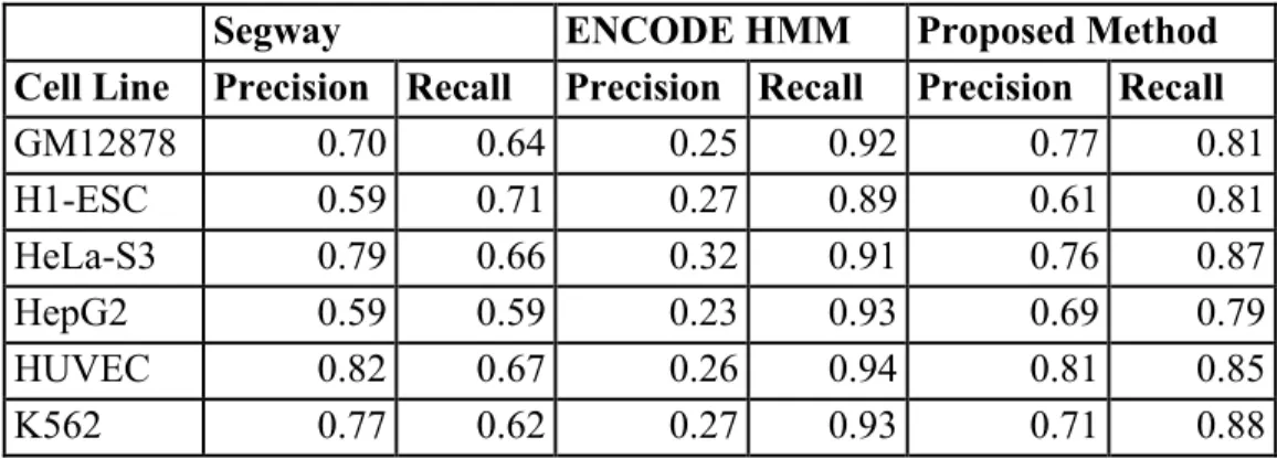
The results of the aforementioned region-finding algorithms depend on read density, and do not classify regions as originating from transcription initiation or confounding biological processes, despite the importance of this. The only algorithm specifically designed to classify CAGE regions is based on modelling nucleotide k-mer frequencies surrounding the regions using an unsupervised hidden Markov model (Djebali et al., 2012), herein called the ENCODE HMM method. Two models are trained. In the first, the k-mers used in training are weighted proportionally to the number of reads in a region. In the second model, all k-mers are weighted equally. The posterior probability of each cluster fitting to the main model is calculated using Bayes’ rule and regions are classified using a threshold on the
probability. In other words, the algorithm biases towards learning the features of CAGE regions with high read counts, and against regions derived from lowly expressed genes. No validation of results from the classifier was performed in the original article. The authors also did not consider integrating external data in their model, which could potentially improve the classifier’s performance. Segway is another method that classifies regions into categories, such as TSS, Enhancer, and Gene End, but does not take CAGE-seq data as input (Hoffman et al., 2012). It is based on dynamicBayesian networks. The simplest
2.1 Background approach that avoids region classification (and region calling) altogether is to make small counting windows around annotated TSS (Plessy et al., 2012), before performing an analysis of the amount of signal, such as differential expression. The drawback is that novel transcription starts, and even novel genes, are ignored.
In summary, the CAGE-seq algorithms proposed previously do not sufficiently model features of the dataset to enable accurate region determination and their classification. The region-finding algorithms either overestimate the size of regions by not properly taking into account the noise distribution or provide millions of mostly overlapping and redundant regions. Also, the region classification algorithms have not been independently evaluated, which may identify possibilities for improvement.
2.1.5 HTS Mapping
Millions of short sequences obtained from the sequencing technologies introduced above must be accurately mapped to a large reference genome in a reasonable amount of time. The large number of reads generated and the size of genomes has motivated the development of fast and accurate algorithms for short sequence mapping. Unlike the classic Needleman-Wunsch algorithm for aligning pairs of sequences, the algorithms developed for HTS data use heuristics to find good matches, but don’t guarantee finding the best match of a sequence to a reference. The earliest of these is Bowtie (Langmead, Trapnell, Pop, & Salzberg, 2009), which uses a Burrows-Wheeler transform and a
Ferragina-Manzini index to align about 25 million sequences per hour. Bowtie is sufficient for mapping CAGE-seq, ChIP-seq, and DNAse-seq data. Most RNA-seq data has special requirements for its
accurate mapping. RNA-seq mapping software needs to be able to map sequences across large gaps, because of introns. Specialised applications for mapping RNA sequences to the genome include TopHat (Trapnell, Pachter, & Salzberg, 2009) and STAR (Dobin et al., 2013), which use similarly efficient data structures and heuristics to Bowtie to map millions of reads in a short amount of time.
2.2 Two-stage Preprocessing Algorithm
To enable biologically valid insights to be derived from CAGE-seq data, a two-stage approach is proposed. In the first stage, a sliding widow is applied across the genome and regions are identified based on comparison to a large number of randomly chosen regions. In the second stage, a linear SVM is applied to predict if the found regions are caused by transcription initiation or biological artefacts.
2.2.1 Region-Finding
In the first stage, a sliding window approach is used to detect regions of significant signal enrichment using a cut-off based on randomly sampled windows. The algorithm starts with background estimation, followed by window joining and region trimming. Assuming that genuine TSS signals are rare in the genome, 1000 candidate windows of width w are generated at random locations in the genome. The CAGE reads within each window are counted and the 95th percentile of the counts is taken as the cut-off
value, below which a window is deemed to have insufficient signal to form a region. Next, a candidate window of width w is moved along each strand of each chromosome in increments of 𝑤/2. Here, 𝑤 = 50 is used, which is typical of regions found previously (Carninci et al., 2006). For each candidate window, the count of CAGE read starts is made. If the count is above the background cut-off value, the window is added to a list of regional windows. The ends of regional windows are trimmed for
outermost, contiguous positions that contain counts less than the cut-off value, divided by the window width. Finally, any adjacent regional windows separated by less than 30 base pairs are merged into a single region.
2.2.1.1 Comparison of Regions
Evaluation is based on publicly available CAGE-seq data of six cell lines (GM12878, H1-hESC, K562, HeLa-S3, HepG2, and HUVEC – the CAGE cell lines). Mapped BAM files were downloaded from the ENCODE data repository (ENCODE Project at UCSC, n.d.) on the UCSC Genome Browser website.
2.2 Two-stage Preprocessing Algorithm Preprocessing details are found elsewhere (Djebali et al., 2012). The unique Submission IDs are 3946, 2380, 2359, 2363, 2381, and 2376 and the number of mapped reads are 19677397, 24604761, 24319886, 24394908, 24604043, and 18717719, respectively.
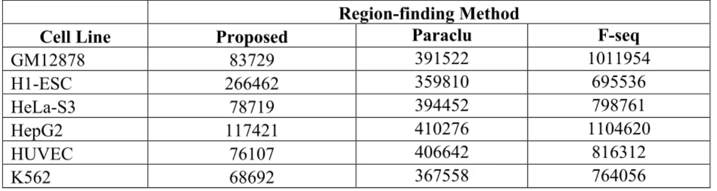
All three algorithms discover tens or hundreds of thousands of regions in each sample (Table 2). The proposed method finds the least number of regions for each cell line. The greatest number of regions are found for the hESC cell line by the proposed method, but HepG2 for the other two methods. H1-hESC is the only stem cell sample in the study; the other five are differentiated cells. F-seq finds over one million regions for GM12878 and HepG2 cells.
Table 2.1 Number of regions detected for each cell line. The proposed sliding window, Paraclu and F-seq are evaluated.
Tabulation of the overlaps of regions between the proposed method with the regions found by Paraclu and F-seq demonstrates that there is a lot of similarity between the regions found by the methods evaluated (Table 2.2). Indeed, every region found by the proposed method is also found by Paraclu. However, a visual exploration of the regions shows that Paraclu and F-seq are detecting many other regions which have minimum support – as little as one CAGE-seq read (Figure A-1) – or they span large regions of the genome, which contain multiple known genes.
Region-finding Method
Cell Line Proposed Paraclu F-seq
GM12878 83729 391522 1011954 H1-ESC 266462 359810 695536 HeLa-S3 78719 394452 798761 HepG2 117421 410276 1104620 HUVEC 76107 406642 816312 K562 68692 367558 764056
Table 2.2 Percentage overlap between proposed method’s regions and those found by Paraclu and F-seq. Regions must have at least one base overlap and be on the same genomic strand to be considered as overlapping.
2.2.2 Classification of Regions
A linear support vector machine (SVM) classifier is developed to classify regions found by the proposed method as TSS or otherwise with high precision and recall. Two kinds of features are calculated for each region; internal features and external features. Internal features are those that may be computed from the CAGE-seq data directly or the genome it is mapped to. External features are derived from associated datasets, such as ChIP-seq or RNA-seq. External features may be further divided into matched and pooled features. Matched features are those that are calculated on the same sample the CAGE-seq is
performed on, whereas pooled features are those calculated from an aggregation of other samples distinct from the sample under consideration. Many features are computed in windows that are a certain distance upstream and downstream of the region’s summit. Definitions of these terms are provided in Section 1.1.
2.2.2.1 Features and Classes
Three internal features are considered:
Kurtosis: Pearson’s kurtosis of the CAGE read histogram of an identified region, based on the fourth standardised moment, is calculated. This feature is analysed to examine if any differences in shape would be discriminatory.
Region-finding Method
Cell Line Paraclu F-seq
GM12878 99.7% 100% H1-ESC 99.8% 100% HeLa-S3 99.7% 100% HepG2 99.8% 100% HUVEC 99.7% 100% K562 99.7% 100%
2.2 Two-stage Preprocessing Algorithm Read density: The number of CAGE reads inside the boundaries of an identified region, divided by the width of the region. This feature is a combination of the shape and height of a region.
4-mer counts: Patterns of DNA bases surrounding the TSSs are also known to be different to other regions in the genome (Sonnenburg, Zien, & Rätsch, 2006). A 500 base pair window was created upstream and another downstream of the summit of each CAGE region. Frequencies of all 4-mers were calculated independently for the two windows. In the upstream window, there are 44 = 256 distinct 4-mers, and similarly downstream, making a total of 512 4-mer features.
Furthermore, five external features are considered. All datasets were downloaded from the ENCODE Project Repository (ENCODE Project at UCSC, n.d.).
Mammalian conservation: Considered for its known association with regulatory regions, such as
promoters, scores within the regions are used. For each region, the conservation values of each base are averaged. A small fraction of regions may not overlap with any bases with conservation scores, because the genomic sequence is not able to be multiply aligned to the other genomes. For these regions, an imputed value, equal to the minimum value of regions that had available conservation scores, is used. TFBS: For each region, the maximum score in a window extending 100 base pairs from the region boundaries is assigned to the region. Rather than exclude cell type-specific signals, the measured maximum is used. Pooled measurements of transcription factor binding from 95 cell types of an unspecified number of transcription factors stored in the table wgEncodeRegTfbsClusteredV2.
DNAse I hypersensitivity: This feature is considered because TSSs typically occur in open chromatin. Similar to TFBS, the maximum count within 100 base pairs from region boundaries is determined. Pooled DNAse I hypersensitivity data using 74 cell lines was obtained from the table named wgEncodeRegDnaseClustered.
H3K4me3: This histone modification is known to be found on the nucleosomes surrounding active TSSs. Again, the maximum score within 100 base pairs of the region boundaries is calculated. Seven files were downloaded with Submission IDs of 2806, 2815, 2846, 2878, 2890, 2909, and 2921.
RNA-seq difference: The number of RNA-seq reads on either side of the region is counted. One count is a 100 base wide flanking window immediately upstream of the 5’ edge of the region. The other is the same size, but downstream of the 3’ edge of the region. The feature calculated is 𝑃(𝑌 ≤ 𝑦) of the Poisson distribution where 𝜆 is equal to the downstream flank count and y is the count in the upstream flank. Unmapped, total RNA-seq data for two of the six CAGE cell lines (GM12878 and K562) was downloaded. Total RNA-seq data is not available for the other four cell lines. The unique Submission IDs are 1502 and 1503. Raw reads were mapped to the human genome assembly hg19 with STAR (Dobin et al., 2013). Only uniquely mapping reads and no more than 3 mismatches to the reference sequence were allowed. 40 bases from the ends of each pair of reads were ignored, as these correspond to stretches of low-quality sequencing data. No splice junctions spanning more than 100000 bases were allowed.
All features are standardised to be between 0 and 1 by dividing by the maximum score for all regions, per feature type and per cell line. A concise overview of all features is provided by Table 2.3.
2.2 Two-stage Preprocessing Algorithm
Table 2.3 Features considered for TSS classification. For each feature, the summarisation procedure, location of data points summarised, and the feature categorisation are shown.
Name Summarisation Location Type
Kurtosis Directly used Region Internal
Read Density Directly used Region Internal
4-mers Counts Count 500 bases upstream
and downstream of region summit
Internal
TFBS Maximum Region and 100 base extension of
boundaries
External Pooled DNAse I
Hypersensitivity Maximum Region and 100 base extension of boundaries External Pooled H3K4me3
Hypersensitivity
Maximum Region and 100 base extension of boundaries
External Pooled Mammalian
Conservation Average Region External Pooled
RNA-seq Difference Distribution function probability
100 bases flanks adjacent to region boundaries
External Matched
The class labels of regions determined by ENCODE HMM were also obtained from the repository, with Submission IDs 5610 and 5147. Five of the cell lines erroneously have the same submission identifier in the database, although manual inspection confirmed that all files do contain sample-specific results. Segway’s labels were downloaded from the supplementary materials website accompanying ENCODE’s analysis of the same six cell lines (Hoffman et al., 2013).
2.2.2.2 Classifier Construction
Unlike typical classification datasets, where the true class membership is known in advance, TSS datasets require the assignment of inferred class labels to regions. Class labelling of regions was made by the same method used for Segway’s evaluation (Hoffman et al., 2012); Segway is, to date, the most comprehensive study of TSS region determination. It involves the use of dynamic Bayesian networks to create a segmentation of the genome, followed by manual assignment of biological categories to the segments by a domain expert. Briefly, 500 bases wide windows were made upstream and downstream of