Intralayer Synchronization in Evolving Multiplex Hypernetworks: Analytical Approach \ast

Intralayer Synchronization in Evolving Multiplex Hypernetworks: Analytical Approach\ast

Sarbendu Rakshit\dagger , Bidesh K. Bera\ddagger , Erik M. Bollt\S , and Dibakar Ghosh\dagger

Abstract. In this paper, we study intralayer synchronization of multiplex networks where nodes in each layer

interact through diverse types of coupling functions associated with different time-varying network topologies, referred to as multiplex hypernetworks. Here, the intralayer connections are evolving with respect to time, and the interlayer connections are stagnant. In this context, an interesting and important problem is to analyze the stability of the intralayer synchronization in such temporal networks. We prove that if the dynamical multiplex hypernetwork for the time-average topology possesses intralayer synchronization, then each layer of the time-varying multiplex hypernetwork will also be synchronized for sufficiently fast switching. Then through master stability function formalism, we analytically derive necessary and sufficient stability conditions of intralayer synchronous states for such temporal architecture in terms of a time-average network. In this regard, we are able to decouple the transverse error component of the intralayer synchronization states for some special cases. Also, we extend our study for nonlinear intralayer coupling functions as well as multilayer hypernetwork architectures. Finally, the theoretical findings are verified numerically by taking the network of paradigmatic chaotic R\"ossler oscillators.

Key words. time-varying network, hypernetwork, multilayer network, synchronization, master stability

func-tion approach

AMS subject classifications. 37A60, 93D05, 93D20, 37D45, 37N20

DOI. 10.1137/18M1224441

1. Introduction. In recent years, the research on complex networks has become an im-mensely active area with the emergence of scientific application over numerous disciplines

[11, 3]. Single complex network architecture can capture the diverse class of subnetworks

in which each subnetwork effects the other networks, and such network structures are called multilayer networks. The intralayer coupling mechanism for each layer may differ from the other layers and also from layer-layer interactions. When each layer has the same number of

\ast

Received by the editors November 2, 2018; accepted for publication (in revised form) by I. Belykh February 5, 2020; published electronically April 23, 2020.

https://doi.org/10.1137/18M1224441

Funding: The third author's research was supported by the Army Research Office (USARO) (N68164-EG),

the Office of Naval Research (ONR) (N00014-15-1-2093), and the Defense Advanced Research Projects Agency (DARPA). The fourth author's research was supported by SERB-DST (Department of Science and Technology), Government of India (project EMR/2016/001039).

\dagger

Physics and Applied Mathematics Unit, Indian Statistical Institute, Kolkata, West Bengal, 700108, India

([email protected],[email protected]).

\ddagger

Department of Mathematics, Indian Institute of Technology Ropar, Punjab - 140001, India, and Physics and

Applied Mathematics Unit, Indian Statistical Institute, Kolkata, West Bengal, 700108, India (bideshbera18@gmail.

com).

\S

Department of Mathematics, Department of Electrical and Computer Engineering, and Department of Physics,

Clarkson University, Potsdam, NY 13699 ([email protected]).

nodes and interlayer connections have one-one correspondence, that is, connecting only the replica nodes of each layer, then the network structure is called a multiplex network.

Re-cently, such networks [10,29] have become a rapidly growing research topic, since it elegantly

furnishes a representation of many realistic systems, such as social networks [54], mobility net-works [14], neural netnet-works [2], subway netnet-works [16], air transportation netnet-works [15], etc., that are appropriately described by this multiplex framework. At the same time, multiplex networks are also supported to describe the several spontaneous processes, such as spreading

of epidemics [47, 21, 13, 46], diffusion processes [20], percolation [12, 8], evolutionary game

dynamics [55], etc. Various type of interactions can be systematically organized into a differ-ent class of network structures. When a set of nodes interacts with the other classes of nodes within the same network through various types of interactions, such network architecture is

calledhypernetworks[50]. Such structural network formation gives us a framework to analyze

the various complex phenomena, which include transportation networks [30], power grids and computer communication networks [12], social interaction networks [31], neuronal networks

[4,27], and coordinated motion of schools of fish [33,1].

The study of synchronization in large-scale complex networks has become an extremely active area across numerous theoretical and applied scientific fields. Different types of

syn-chronization phenomena [44,42], such as interlayer synchronization [48], intralayer

synchro-nization [17] in multiplex networks, and cluster synchrosynchro-nization [9] in multilayer networks, are studied. To analyze the stability of the synchronization state in static multilayer networks, a

general method has recently been proposed in [5]. A few studies [50,43,26] have been

per-formed on the hypernetwork (i.e., networks with multiple kinds of couplings between nodes of the same type) in the monolayer situation. Instead, the case of networks formed by nodes of different types (where all the nodes of the same type form a ``group"") has been studied in [51]. In both of the mentioned cases of different couplings types and different nodes types, a dimen-sionality reduction was obtained, which led to a master stability function (MSF) solution of the stability problem, similar to the original approach in [36]. With the help of this approach, Sorrentino [50] analytically and numerically investigated the stability of the global synchro-nization state in a static monolayer hypernetwork consisting of different types of network Laplacians. In the case of [26], the dimensionality reduction was obtained by using simultane-ous block diagonalization of matrices. By this dimensional reduction, necessary and sufficient conditions for the stability of the synchronous solution can be easily obtained. However, all of these synchronization phenomena were usually studied in completely time-static networks, which means the underlying interaction topology is time-invariant. The time-varying features

are ubiquitous in many natural and real-life networks [56, 32, 34, 49, 45], where the links

between the nodes are created, destroyed, or rewired over various time-scales [25].

Reference [52] provides a new fast switching stability criterion, which gives sufficient con-ditions for a temporal network to behave in unison and thus contributes a new insight about the stability analysis of a time-varying network. Let there be a new description of connectivity, the time-average graph Laplacian; then its spectral property employed with master stability

formalism accurately predicts synchronization. The connection graph stability method [6, 7]

also analyzes the stability of synchronization for time-varying networks. This method is rooted explicitly in graph theory, based on the total length of all paths through edges on the

fast switching, the time-varying system exhibits a stable synchronous solution whenever it is stable in the corresponding time-average system. In those previous works, the analytical studies were restricted to only the simple scalar diffusive types of interaction functions, but the coexistence of the different types of coupling functions was not discussed.

The stability of synchronization was analyzed stochastically for a group of dynamic agents that communicate via a moving neighborhood network [41] by introducing the concept of a ``long-time expected communication network."" It was shown that if the long-time expected net-work supports synchronization, the stochastic netnet-work will also synchronize when the agents communicate sufficiently fast within the network. Porfiri, Stilwell, and Bollt [40] studied the synchronization in a stochastic time-varying network, and it could be possible even if the network is not always connected but the expected network is connected for sufficiently fast switching. Global synchronization was also studied in coupled chaotic systems with randomly intermittent coupling [39] using partial averaging techniques and stochastic Lyapunov stability theory for sufficiently small switching periods. The theoretical findings of the fast switching stability criterion are also experimentally verified in coupled Chua's circuits with master-slave configuration [38]. If the blinking system switches fast enough, then a solution of the blinking system closely follows the solution of the average system for a finite time interval. Afterward, they drift apart [22]. The explicit bounds of that time interval that relate the probability, the switching frequency, the precision, and the length of the time interval to each other can also be found. In a follow-up paper, the asymptotical properties of general blinking systems with identically distributed independent random switching variables were also studied [23]. The un-expected windows of synchronization for moderate switching frequencies were noticed in [28], in which synchronization in the switching network becomes stable even though it is unstable in the average network for fast switching. Later, the stability of the global synchronization

for nonfast switching networks was studied in [37,18].

Inspired by the above facts, we study the intralayer synchronization in time-varying mul-tiplex hypernetworks. Here each link corresponding to the intralayer interaction function is allowed to switch stochastically with respect to time with a certain rewiring frequency, while the layer-layer connectivity is stagnant over time. Through the fast switching stabil-ity criterion, we first prove the stabilstabil-ity of the intralayer synchronization for time-average multiplex hypernetworks, implying the stability of the corresponding time-varying network. Through the master stability function theory, we derive necessary and sufficient conditions for the intralayer synchronization state, and correspondingly we enunciate the validity of the time-average system. Moreover, the master stability equations can be decoupled if only one of the time-average Laplacian matrices commutes with all other matrices. We show that the spectrum of the time-average intralayer graph Laplacian precisely predicts the stability of the intralayer synchronization. We also extend the stability theory for intralayer synchronization for multilayer hypernetworks and also for nonlinear intralayer coupling functions. To verify

our analytical findings, we use a paradigmatic chaotic system, namely the R\"ossler

oscilla-tor as the node dynamics in each layer, and we explore the parameter regions for intralayer synchronization.

2. Background materials. In this section, we give some preliminaries that are essential for this work, especially on basic graph theory on hypernetworks, the master stability function

approach for a static network, and the notion of the fast switching stability criterion of a time-varying system.

We denote the set \{ k, k+ 1, . . . , N\} by Nk, where k, N \in \BbbN . For a square matrixA, Atr

and A\ast respectively denote the transpose and Hermitian of that matrix.

Here\otimes denotes the matrix Kronecker product. A few standard properties of the Kronecker product for square matrices are utilized here, stated as follows [19]:

1. (A\otimes B)(C\otimes D) = (AC)\otimes (BD), 2. (A\otimes B)tr _=Atr_{\otimes B}tr_,

3. (A\otimes B) - 1 =A - 1\otimes B - 1.

Throughout our manuscript, Op\times q denotesp\times q zero matrix, andIp is thep\times pidentity

matrix.

2.1. Graph theoretical characterization. Various types of interactions can be systemat-ically organized into classes of network structures. Mathematsystemat-ically, a complex network is a

pairG = (X, E), whereX is the set of vertices and E denotes the set of edges connecting the

vertices, using classical graph theory.

A multilayer network is a pairM = (G,C), whereG =\bigl\{

G\beta = (X\beta , E\beta ) :\beta \in \{ 1,2, . . . , L\}

\bigr\}

is a family of graphs each representing a layer and C = \bigl\{

E\beta 1\beta 1 \subseteq X\beta 1 \times X\beta 2 : \beta 1, \beta 2 \in \{ 1,2, . . . , L\} , \beta 1 \not =\beta 2

\bigr\}

is the set of interconnections between nodes of nonidentical layersG\beta 1

and G\beta ₂. The elements ofE\beta are intralayer connections, and elements of C are called crossed

layers, where all elements of E\beta 1\beta 2 are the interlayer connections. A multiplex network is a

special type of multilayer network, in which each layer has the same number of nodes and interlayer connections of a given node that connect only to its counterpart nodes in the rest

of the layers. In other words, for a multiplex network | X₁| = | X₂| = \cdot \cdot \cdot = | X_L| = N and

E\beta 1\beta 2 = \bigl\{ \bigl( v[\beta 1] i , v [\beta 2] i \bigr) , i\in N1 :v[\beta 1] i \in X\beta 1, v [\beta 2] i \in X\beta 2 \bigr\}

,| \cdot | denotes the cardinality of a set.

Consider a family of networksG[\alpha ]=\bigl( X, E[\alpha ]\bigr) ,\alpha = 1,2, . . . , M, whereXis the fixed set of

nodes for each\alpha , andE[\alpha ]\subseteq X\times Xis a nonempty set of edges. IfE=\bigl\{ E[\alpha ]:\alpha = 1,2, . . . , M\bigr\}

is the family of links, then a hypernetwork is a pairH = (X, E). Here eachE[\alpha ]corresponds

to the various modes of interaction. We call each of these atier.

Definition 2.1. A multilayer hypernetwork is an ordered pair M_H = (G,C), where G =

\bigl\{

G\beta = (X\beta , E\beta ) : \beta \in \{ 1,2, . . . , L\}

\bigr\}

are the family of graphs, each representing a layer, in which E\beta =

\bigl\{

E_\beta [\alpha ] : \alpha \in \{ 1,2, . . . , M\} \bigr\}

are the family of hyperlinks for each tier \alpha .

C =\bigl\{ E\beta 1\beta 2 \subseteq X\beta 1\times X\beta 2 :\beta 1, \beta 2 \in \{ 1,2, . . . , L\} , \beta 1 \not =\beta 2 \bigr\}

is the set of interlayer connections between nodes of nonidentical layers G\beta ₁ and G\beta ₂.

A complex networkG = (X, E) is described as time-varying ifG =G(t) depends explicitly

on timet, i.e., both X =X(t) and E =E(t) are functions of time. This includes the case in

which the switching between the edgesE(t) varies as the graph evolves, where the set of nodes,

X, is time-invariant. The time-varying networks are therefore characterized by the adjacency

matrices that undergo such abrupt changes. Such a time-varying network G(t) =\bigl( X, E(t)\bigr)

will be described as jointly connected if the union of its frozen time networks\bigl( X,\cup _tE(t)\bigr)

con-stitutes a connected graph. For complete synchronization to occur, the underlying temporal network should be jointly connected.

the network is a function of time, but the interlayer connectionC is time-invariant.

Definition 2.2. The time-stamped multilayer hypernetwork M_H(t) is jointly connected if

the union of its frozen-time projected network\bigl( \cup L

\beta =1X\beta , \cup t\cup M\alpha =1\cup L\beta =1E [\alpha ] \beta (t)\cup C

\bigr)

constitutes a connected graph.

To achieve complete intralayer synchronization, it should be jointly connected. In a frozen

time, any tier\bigl( X, E[\alpha ]\bigr) may have one or more disconnected components, but the frozen-time

projected network should be connected.

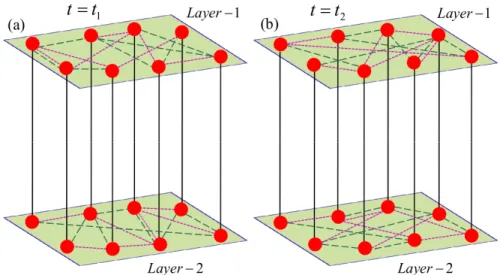
Figure 1. Schematic of time-varying interactions in a hypernetwork with a multiplex formation at two

different time instants: (a) t1 and (b) t2. Each node is represented by a red solid circle. The green dashed and magenta dotted lines denote the different types of interactions of the hypernetwork, while the interlayer connections between the layer are denoted by solid black lines.

The schematic diagram (Figure 1) represents the time-varying interaction in a

hyper-network with the multiplex structure of two layers consisting of N = 8 nodes and M = 2

interaction types in each layer. Two different types of interacting tiers are shown for two

particular instances of times t = t1 and t = t2 in Figures 1(a) and 1(b), respectively. Here

the links of one tier are denoted by the green dashed lines and the other one by magenta dotted lines, whereas the interlayer connections between the layers are represented by black solid lines.

2.2. Review of master stability function approach. From the dynamical system's per-spective, an important question arises on when a synchronization state of a network of coupled oscillators is stable, regarding the coupling strength. The MSF approach [36] analyzes the stability of the synchronization state of primarily identically coupled oscillators. Also, the stability condition for synchronization using the MSF approach in the coupled nearly identi-cal systems has been extended [53]. This approach assumes that all the coupled oscillators are identical and the synchronization manifold is invariant, to guarantee the existence of a synchronous solution. Here the coupling function for each link is same and should vanish after achieving the synchronization, to make the specific stability diagram.

Consider a network consisting of N identical oscillators, where xi is the d-dimensional

state vector of the ith node, with its autonomous evolution \.xi =F(xi). We assume that the

dynamics of the entire network can be written as

(2.1) x\.i=F(xi) - \epsilon

N

\sum

j=1

LijBxj,

where \epsilon is the coupling strength, B \in _\BbbR d\times d _{determines through which variables the N}

oscil-lators are coupled, andL is the network Laplacian.

When complete synchronization occurs, all the oscillators evolve synchronously withxi =

x0. Perturbation to the ith oscillator from its synchronization manifold is by \delta xi. Letting

\delta x= [\delta xtr₁, \delta xtr₂, . . . , \delta xtr_N]tr, the variational equation of (2.1) near its synchronization manifold

x0(t) can be written as

(2.2) \delta x\. =\bigl[ IN \otimes J F(x0) - \epsilon L \otimes B

\bigr] \delta x.

The synchronous state is said to be locally stable if for any small perturbation \delta xi each

oscillator asymptotically converges to the synchronization manifold, i.e., xi \rightarrow x0 as t\rightarrow \infty ,

which implies that\delta xi\rightarrow 0 ast\rightarrow \infty fori\in N1. In other words, the trivial equilibrium point

of (2.2) is asymptotically stable. However, (2.2) contains information regarding the parallel component of the synchronization error vector, as well as the transverse components, while the synchronization solution will be asymptotically stable only if the latter components are damp-out, and conversely. Therefore, to analyze the stability of the synchronous solution, we should

concentrate on the stability of the variations\delta xi which are transverse to the synchronization

manifold. So we have to separate out the parallel component from (2.2).

The Laplacian matrixL is a real valued square matrix; furthermore, for the bidirectional

coupling, it is symmetric. As we know, every square matrix is unitarily triangularizable by

its basis of eigenvectors. So there exists a matrix P \in MN(\BbbC ) such that U = P - 1LP

is a triangular matrix, where the columns of P are the orthonormal eigenvectors of L and

P\ast P =P P\ast =IN. The principal diagonal elements\{ \gamma 1, \gamma 2, . . . , \gamma N\} ofU are the eigenvalues

ofL. In the context of synchronization, it is assumed that the underlying network is connected

as a minimal condition of synchronizability. Hence, exactly one eigenvalue of L is zero (say,

\gamma 1 = 0) and the other eigenvalues \gamma i \in \BbbC for alli\in N2. Now consider the Schur transformation

(2.3) \xi (t) = (P\otimes Id) - 1\delta x(t).

Applying (2.2), we have

(2.4) \xi \.(t) =\bigl[

IN \otimes J F(x0) - \epsilon U\otimes B)

\bigr] \xi (t).

For the block diagonal structure ofIN\otimes J F(x0) and the block triangular form ofU \otimes B, the

stability of (2.4) is equivalent to the stability of the followingN uncoupled systems:

(2.5) \xi \.i(t) =

\bigl[

J F(x0) - \epsilon \gamma iB)

\bigr]

Fori= 1, the variational equation becomes \.\xi 1(t) =J F(x0) \xi 1(t). But it is the linearized

equation of the synchronization dynamics \.x0 = F(x0). Thus it evolves along the parallel

to the synchronization solution, which we want to eliminate. For i \in N2, the variational

equation (2.5) evolves transversally to the synchronization manifold. This dimensionality reduction allows us to easily calculate the Lyapunov exponents of the decoupled transverse error systems for the stability of the synchronization state.

The synchronization state will be stable if all the eigenmodes are stable for the given

coupling strength. Then the maximum Lyapunov exponent \Lambda maxof the transverse variational

equations reveals the stability of the synchronization state. If \Lambda max(\epsilon )>0 for some coupling

strength \epsilon , then the system (2.5) diverges, which indicates that the system (2.4) is

asynchro-nous. By increasing \epsilon , if \Lambda max becomes negative, then we will get stable synchronization.

Now we can associate a function \Lambda max(\epsilon ) :\BbbR \rightarrow \BbbR with transverse eigendirections (2.5) as a

function of the coupling strength \epsilon , which returns the maximum Lyapunov exponent among

all transverse directions. That is why this stability analysis was coined as themaster stability

function approach [36]. Hence, by the MSF approach, the coupling strengths for which the

dynamical network evolves synchronously can be computed for astatic network.

2.3. Review of the fast switching stability criterion. For a temporal network, the un-derlying Laplacian matrix changes with respect to time. Therefore, its eigenvalues and corre-sponding eigenvectors are functions of time. So the span of the basis of eigenvectors changes whenever the Laplacian matrix changes. However, to eliminate the parallel error component from the entire error dynamics, we should project the error components to a unique space. So the Schur transformation (2.3) and the MSF cannot be applied directly in the case of a time-varying network. To compromise with this difficulty, Stilwell, Bollt, and Roberson [52] introduced the fast switching stability criterion for time-varying networks. To get an overview of the stability of temporal graphs, we briefly review some of these details.

Fast switching indicates that the time-scale of the network evolution is faster than the time-scale of the coupled oscillators. The stability analysis of this paper is based on the fast switching stability technique. It provides new insights about the stability of dynamical systems when the underlying network is time-varying. Before describing this technique, we need the following preliminary lemma, which was proved in [52].

Lemma 2.3. If there exists a time-average matrix E\= of the matrix valued function E(t)

such that

1

T

\int t+T

t

E(\tau ) d\tau = \=E \forall t\in \BbbR + and for some constant T,

then for sufficiently fast switching, the system

(2.6) z\.(t) =\bigl[

A(t) +E(t)\bigr]

z(t), z(t0) =z0, t\geq t0,

will be uniformly asymptotically stable whenever the time-average system

(2.7) x\.(t) =\bigl[

A(t) + \=E\bigr]

x(t), x(t0) =x0, t\geq t0,

Herez0andx0are two independent different initial conditions from the basin of attraction

of the asymptotically stable state of systems (2.6) and (2.7), respectively. However, this

lemma works for any constant time t, but for sufficiently large time T, it depends on A(t)

and how fast E(t) is switching. The stability of the frozen time system does not guarantee

the stability of the switched system, but this lemma shows that the switched time-varying system can be asymptotically stable if for sufficiently fast switching, the time-average system is asymptotically stable.

Now consider a temporal network ofN identical coupled oscillators

(2.8) x\.i(t) =F(xi(t)) - \epsilon

N

\sum

j=1

Lij(t) B xj(t),

wherei\in N1 and L(t) is the time-varying graph Laplacian.

For sufficiently fast switching, the time-average Laplacian matrix L\= satisfies

\= L = 1 T \int t+T t L(\tau ) d\tau

for some constant T. The matrix L\=has the same inherent zero-row sum property from the

parent Laplacian L(t). But L\=may not necessarily describe any particular network; rather

it is just the term by term time-average of the time-varying graph Laplacian L(t).

The real square matrix L\= can be unitarily triangularizable. Then we can construct a

unitary matrix P with each column representing the orthonormal eigenvectors of L\=, such

that P - 1L\=P = \=U = \biggl[ 0 U\=1 ON - 1\times 1 U\=2 \biggr]

is the Schur transformation of L\=.

Here \=U2\in MN - 1(\BbbC ) is an upper triangular matrix with principal diagonal elements asN - 1

eigenvalues of \=L excluding 0. The equation of motion of the coupled system incorporating the

above average Laplacian will be obtained from (2.8) just by replacingL(t) by \=L. Considering

the Schur transformation and using the unitary matrix P, the equation of the error system

transverse to the synchronization manifold can be written as

(2.9) \eta \.(t) =\bigl[

IN - 1\otimes F(x\bfzero (t)) - \epsilon U\=2\otimes B

\bigr] \eta (t).

By considering the same Schur transformation applied to (2.8), the equation of motion of the transverse error system becomes

(2.10) \xi \.(t) =\bigl[ IN - 1\otimes F(x\bfzero (t)) - \epsilon U2(t)\otimes B

\bigr] \xi (t), where P - 1L(t)P = \biggl[ 0 U1(t) ON - 1\times 1 U2(t) \biggr]

is the Schur transformation ofL(t).

Now it is easy to produce \= U1 = 1 T \int t+T t U1(\tau ) d\tau .

Thus, by applying Lemma2.3, we can conclude that if the time-average system has an asymp-totically stable synchronization manifold, then the time-varying network also possesses an asymptotically stale synchronous solution for sufficiently fast switching. This fast switching stability criterion will be used to assess the local stability of the intralayer synchronization state.

3. Mathematical model. We now consider a coupled multiplex dynamical network, where different types of interactions are simultaneously present in each layer. With this network architecture, here for the first time, we rigorously analyze the stability of the intralayer syn-chronization state. In each layer, individual dynamical systems are coupled through more than one distinct connection, each of which corresponds to different types of interactions.

We start by considering two layers, each composed of N nodes of d-dimensional identical

dynamical systems. In each layer, N nodes are interacting through M different tiers of

con-nections, which represent different kinds of couplings among themselves. The states of the

layers are represented by the vectors x = \{ x1,x2, . . . ,xN\} and y = \{ y1,y2, . . . ,yN\} with

xi,yi \in \BbbR d. Then the mathematical form of the general time-varying multiplex hypernetwork can be represented as (3.1) \. xi=F1(xi) - M \sum \alpha =1 \epsilon \alpha N \sum j=1 L[1,\alpha ] ij (t)G [1] \alpha (xj) +\lambda H1(xi,yi), \. yi=F2(yi) - M \sum \alpha =1 \epsilon \alpha N \sum j=1 L[2,\alpha ] ij (t)G [2] \alpha (yj) +\lambda H2(yi,xi),

wherei\in N1. HereF1,2 :\BbbR d\rightarrow \BbbR dandH1,2 :\BbbR d\times \BbbR d\rightarrow \BbbR dare the continuously differentiable

functions which respectively represent the autonomous evolution of the uncoupled oscillator and the output vectorial function between the layers. The individual dynamics within the

same layer are identical but are different for nodes in different layers. Here Hl(x,y) is

dif-ferent from Hl(y,x) for l = 1,2. G

[l]

\alpha : \BbbR d \rightarrow \BbbR d is the vector field of the output vectorial

function within the layers for tier\alpha in layer-l. It is clear that the intralayer coupling functions

corresponding to tier\alpha differ for the two different layers. \epsilon \alpha is the intralayer coupling strength

for tier \alpha , which determines how the information is distributed between nodes through

dif-ferent coupling configurations. The parameter \lambda , interlayer coupling strength, controls the

interaction between the two layers.

The time-varying intralayer network configuration corresponding to the graph\bigl( Xl, E

[\alpha ]

l (t)

\bigr)

is encoded by the N\times N adjacency matrixA[l,\alpha ](t) which describes the interconnections

be-tween individual oscillators for tier\alpha in thelth layer. Here A_ij[l,\alpha ](t) = 1 if (vi, vj)\in El[\alpha ](t),

i.e., theith node and thejth node of the layer-lare connected in tier\alpha at timetand zero

other-wise. L[l,\alpha ](t) is the corresponding zero-row sum graph Laplacian, obtained from the adjacent

matrices A[l,\alpha ](t). The diagonal elementL_ii[l,\alpha ](t) is the sum of the nondiagonal elements in

theith row ofA[l,\alpha ](t), and the off-diagonal elements are the negatives of the corresponding

elements inA[l,\alpha ]_{(t), i.e.,L}[l,\alpha ]

ij (t) = - A [l,\alpha ] ij (t) if i\not =j and L [l,\alpha ] ii (t) = \sum N j=1A [l,\alpha ] ij (t).

Now the intralayer links of the network\bigl( Xl, E[_l\alpha ](t)

\bigr)

vary over time by rewiring the entire

time t and integration time step dt, we rewire each tier in the two layers independently, by

constructing a new network with probability f dt. Large f indicates very fast switching of

links, implying that the networks change rapidly, whereas small f implies that the two layers

are almost static, as the links have a very low probability of change. Each of these successively created networks will be structurally equivalent due to the choice of fixed parameter values throughout the procedure. We are assuming that the intralayer network topologies

corre-sponding to tier \alpha for both of the two layers are exactly identical. However, at a particular

time instant, their adjacency matrices will not generally be equal due to the time-varying connectivity nature of the edges for each tier. On the other side, the interlayer connections are complete multiplex structured and static over time. We assert this as a sufficiently gener-alized model as a multiplex hypernetwork, which allows enough connectionism for intralayer synchronization, and also admit a complete rigorous analysis.

In this paper, our principal contribution is to show, for temporal (sufficiently fast) in-tralayer network topologies, that each layer can synchronize if in the time-average network, each layer possesses stable complete synchronization.

4. Main results. In complete intralayer synchronization, each individual layer converges on the same time evolution, which occurs when individual oscillator in each layer of a multiplex networks is appropriately coupled. At the intralayer synchronization state, let layer-1 evolve

synchronously with xi = x0 and layer-2 with yi = y0 for all i \in N1. The dynamics of the

synchronization solution\bigl(

x0(t),y0(t) \bigr) can be written as (4.1) x0\. =F1(x0) +\lambda H1(x0,y0), \. y0=F2(y0) +\lambda H2(y0,x0).

Definition 4.1. The multiplex network (3.1) is said to achieve the complete intralayer

syn-chronization state if the two solutions x0(t),y0(t) \in _\BbbR d _{satisfy the equation of motion (4.1)}

such that for all i\in N1,

\| xi(t) - x0(t)\| \rightarrow 0 and \| yi(t) - y0(t)\| \rightarrow 0 as t\rightarrow \infty .

Consequently, the intralayer synchronization manifold can be defined as

\scrS =\bigl\{

(x0(t),y0(t))\subset \BbbR 2d : xi(t) =x0(t), yi(t) =y0(t), i= 1,2, . . . , N and t\in \BbbR +\bigr\} . Its evolution equation is dominated by (4.1). The intralayer synchronization can be observed physically if this manifold is stable with respect to the perturbations in the transverse

sub-space. Now we delve into the stability of\scrS for the temporal multiplex hypernetwork (3.1).

Perturb the ith node in layer-1 from its synchronization manifold x0 with an amount

\delta xi(t) and theith node in the layer-2 with an amount\delta yi(t). So the current state of the ith

node in each layer isxi(t) =x0(t) +\delta xi(t),yi(t) =y0(t) +\delta yi(t) fori\in N1. Linearizing each

in vectorial form yield

(4.2)

\delta x\. =IN\otimes J F1(x0)\delta x - M

\sum

\alpha =1

\epsilon \alpha L[1,\alpha ](t)\otimes J G[1]_\alpha (x0)\delta x

+\lambda \Bigl[ IN\otimes J H1(x0,y0)\delta x+IN \otimes DH1(x0,y0)\delta y

\Bigr] , \delta y\. =IN \otimes J F2(y0)\delta y -

M

\sum

\alpha =1

\epsilon \alpha L[2,\alpha ](t)\otimes J G[2]_\alpha (y0)\delta y

+\lambda \Bigl[

IN\otimes J H2(y0,x0)\delta y+IN \otimes DH2(y0,x0)\delta x

\Bigr] ,

where\delta x(t) =\bigl[ \delta x1(t)tr, \delta x2(t)tr, . . . , \delta xN(t)tr

\bigr] tr

and\delta y(t) =\bigl[ \delta y1(t)tr, \delta y2(t)tr, . . . , \delta yN(t)tr

\bigr] tr

.

Here J and D are the Jacobian operators with respect to the first and second variables,

re-spectively, i.e., J H(x0,y0) = \partial H_\partial (\bfx _\bfx ,\bfy )| (\bfx ,\bfy )=(\bfx 0,\bfy 0) andDH(x0,y0) = \partial H_\partial (_\bfy \bfx ,\bfy )| (\bfx ,\bfy )=(\bfx 0,\bfy 0).

Now consider that each varying intralayer network topology possesses a static

time-average network for sufficiently fast rewiring. Since the network topologies of tier\alpha in both of

the layers are the same, their time-averaged Laplacian matrices will match. Then there exists

a constant T such that

1

T

\int t+T

t

L[l,\alpha ]_{(\tau ) d\tau = \=L}[\alpha ] _{for l= 1,2 and\alpha = 1,2, . . . , M.}

These time-average Laplacian matrices are the indicator of the intralayer synchronization

state. All of them are zero-row sum real square matrices. Their spectrum will be used

to analyze the stability of the error system (4.2). By assuming these average matrices are

connected, exactly one eigenvalue \gamma ₁[\alpha ] is zero, and the other eigenvalues \gamma _i[\alpha ] \in \BbbC , i \in N2.

Also, L\=[\alpha ] can be unitarily triangularized by V[\alpha ], where V[\alpha ] is a unitary matrix. Its ith

column is the eigenvector ofL\=[\alpha ] corresponding to the eigenvalue \gamma _i[\alpha ], and all columns form

orthogonal bases of \BbbC N. Without loss of any generality, consider the first column of V[\alpha ]

to be \bigl( \surd 1 N, 1 \surd N, . . . , 1 \surd N \bigr) tr

corresponding to the eigenvalue zero. Then there exists an upper

triangular matrix \=U[\alpha ] over the field \BbbC such that \=U[\alpha ] = V[\alpha ]

- 1 _\=

L[\alpha ]_V[\alpha ] _{with its principal}

diagonal elements being the eigenvalues of L\=[\alpha ].

Theorem 4.2. The time-varying hypernetwork with multiplex formation whose dynamics

are described by (3.1) possesses intralayer synchronization whenever the corresponding time-average static multiplex hypernetwork

(4.3) \. wi =F1(wi) - M \sum \alpha =1 \epsilon \alpha N \sum j=1 \= L[\alpha ] ij G [1] \alpha (wj) +\lambda H1(wi,zi), \. zi=F2(zi) - M \sum \alpha =1 \epsilon \alpha N \sum j=1 \= L[\alpha ] ij G[2]\alpha (zj) +\lambda H2(zi,wi)

Proof. We first derive the equation of motion of the error system transverse to the in-tralayer synchronization manifold, for both the time-varying and the time-average systems (3.1) and (4.3), respectively.

Taking the time-average intralayer networks, (4.3) is the dynamics of the time-average

multiplex hypernetwork, wherewi (zi) is the state variable of the ith node in layer-1

(layer-2). This time-average system seems to be a notion of average information propagation in a network. Now it is clear that the equation of motion of the intralayer synchronization manifold for the time-varying and time-averaged networks is the same. So, without loss of generality, we can assume that when intralayer synchronization occurs, layer-1 evolves synchronously with

wi=x0and layer-2 withzi =y0for alli\in N1. If\delta w(t) =

\bigl[

\delta w1(t)tr, \delta w2(t)tr, . . . , \delta wN(t)tr

\bigr] tr

and\delta z(t) =\bigl[ \delta z1(t)tr, \delta z2(t)tr, . . . , \delta zN(t)tr

\bigr] tr

are the corresponding perturbations for both of the layers, then the vectorial forms of the error dynamics for intralayer synchronization states of the time-averaged system (4.3) are as follows:

(4.4)

\delta w\.(t) =IN \otimes J F1(x0)\delta w - M

\sum

\alpha =1

\epsilon \alpha L\=[\alpha ]\otimes J G[1]\alpha (x0)\delta w

+\lambda \Bigl[ IN\otimes J H1(x0,y0)\delta w+IN \otimes DH1(x0,y0)\delta z

\Bigr] , \delta z\.(t) =IN \otimes J F2(y0)\delta z -

M

\sum

\alpha =1

\epsilon \alpha L\=[\alpha ]\otimes J G[2]\alpha (y0)\delta z

+\lambda \Bigl[

IN\otimes J H2(y0,x0)\delta z+IN\otimes DH2(y0,x0)\delta w

\Bigr] .

The linearized set of (4.4) can be decomposed into two components: one evolves along the synchronization manifold, and the other transverses to it. If the latter components are asymptotically stable, then the set of oscillators (4.3) will exhibit the stable intralayer

syn-chronization state [35]. To find the transverse error system, we spectrally decompose \delta w(t)

and\delta z(t) of the above equation and project it onto the basis of eigenvectorV[1] corresponding to the first tier. However, the choice of the matrix of eigenvectors is arbitrary, since all of

them form M equivalent bases of\BbbC N.

Under this Schur transformation onto the space spanned by the basis of eigenvectors

of L\=[1]_{, let \delta w(t) and \delta z(t) transform to \eta} (\bfw )_{(t) =} \bigl[

\eta ₁(\bfw )tr(t), \eta ₂(\bfw )tr(t), . . . , \eta _N(\bfw )tr(t)\bigr] tr

and

\eta (\bfz )(t) = \bigl[ \eta ₁(\bfz )tr(t), \eta (₂\bfz )tr(t), . . . , \eta _N(\bfz )tr(t)\bigr] tr, respectively, where \eta (\bfw ) = \bigl( V[1] \otimes Id

\bigr) - 1

\delta w and

\eta (\bfz ) =\bigl( V[1]\otimes Id

\bigr) - 1

\delta z. Using this Schur transformation, the linearized equation (4.4) corre-sponding to the time-average network becomes

(4.5)

\.

\eta (\bfw )(t) =IN\otimes J F1(x0)\eta (\bfw ) - M

\sum

\alpha =1

\epsilon \alpha

\Bigl(

V[1] - 1L\=[\alpha ]V[1]\Bigr) \otimes J G[1]_\alpha (x0)\eta (\bfw )

+\lambda \Bigl[ IN \otimes J H1(x0,y0)\eta (\bfw )+IN \otimes DH1(x0,y0)\eta (\bfz )

\Bigr] ,

\.

\eta (\bfz )(t) =IN \otimes J F2(y0)\eta (\bfz ) - M

\sum

\alpha =1

\epsilon \alpha

\Bigl(

V[1] - 1L\=[\alpha ]V[1]\Bigr) \otimes J G[2]_\alpha (y0)\eta (\bfz )

+\lambda \Bigl[

IN \otimes J H2(y0,x0)\eta (\bfz )+IN \otimes DH2(y0,x0)\eta (\bfw )

\Bigr] .

Since L\=[\alpha ] is unitarily triangularizable andV[\alpha ] - 1L\=[\alpha ]V[\alpha ]= \=U[\alpha ], therefore we have

(4.6) V[1] - 1L\=[\alpha ]V[1] =V[1] - 1V[\alpha ] U\=[\alpha ]V[\alpha ] - 1V[1].

Consider V[\alpha ]= \left[ ₁ \surd N v [\alpha ] 12 v [\alpha ] 13 . . . v [\alpha ] 1N 1 \surd N v [\alpha ] 22 v [\alpha ] 23 . . . v [\alpha ] 2N . . . . 1 \surd N v [\alpha ] N2 v [\alpha ] N3 . . . v [\alpha ] N N \right] .

NowV[\alpha ] is the unitary matrix of orthogonal eigenvectors ofL\=[\alpha ], soV[\alpha ] - 1=V[\alpha ]\ast . Hence,

we can write

V[1] - 1V[\alpha ]=

\left[

1 0 0 . . . 0

0 v₂₂[1,\alpha ] v₂₃[1,\alpha ] . . . v[1_2N,\alpha ] . . . .

0 v_N[1,\alpha ₂] v_N[1,\alpha ₃] . . . v[1_{N N},\alpha ] \right]

and V[\alpha ] - 1V[1] =

\left[

1 0 0 . . . 0

0 v₂₂[\alpha ,1] v₂₃[\alpha ,1] . . . v[₂\alpha ,_N1] . . . .

0 v_N[\alpha ,₂1] v_N[\alpha ,₃1] . . . v[_{N N}\alpha ,1] \right]

.

Making the above substitutions in (4.6), we get

(4.7) V[1] - 1L\=[\alpha ]V[1]= \left[ 0 U\=₁[\alpha ] ON - 1\times 1 U\=₂[\alpha ] \right] ,

where \=U₂[\alpha ]\in \BbbC N - 1\times N - 1 and \=U1[\alpha ]\in \BbbC 1\times N - 1.

The transform variables \eta (\bfw )(t) and \eta (\bfz )(t) yield the decomposition \eta (\bfw ) = \bigl[

\eta _P(\bfw ), \eta _T(\bfw )\bigr]

and \eta (\bfz ) =\bigl[

\eta _P(\bfz ), \eta _T(\bfz )\bigr]

, where\eta _P(\bfw ), \eta _P(\bfz ) \in _\BbbC d _{and \eta} (\bfw )

T , \eta (\bfz )

T \in \BbbC d(N - 1). Making these decom-positions in (4.5) and with the help of (4.7), we get

\.

\eta (_P\bfw )=J F1(x0)\eta (_P\bfw ) - M

\sum

\alpha =1

\epsilon \alpha U\=1[\alpha ]\otimes J G[1]\alpha (x0)\eta (\bfw ) T +\lambda \Bigl[ J H1(x0,y0)\eta (_P\bfw )+DH1(x0,y0)\eta (_P\bfz ) \Bigr] , (4.8a) \.

\eta (_T\bfw )=IN - 1\otimes J F1(x0)\eta _T(\bfw ) - M

\sum

\alpha =1

\epsilon \alpha U\=2[\alpha ]\otimes J G[1]\alpha (x0)\eta (\bfw ) T (4.8b)

+\lambda \Bigl[

IN - 1\otimes J H1(x0,y0)\eta _T(\bfw )+IN - 1\otimes DH1(x0,y0)\eta (_T\bfz )

\Bigr] , \. \eta _P(\bfz )=J F2(y0)\eta (P\bfz ) - M \sum \alpha =1

\epsilon \alpha U\=1[\alpha ]\otimes J G\alpha [2](y0)\eta (T\bfz )+\lambda

\Bigl[ J H2(y0,x0)\eta P(\bfz )+DH2(y0,x0)\eta (P\bfw ) \Bigr] , (4.8c) \.

\eta _T(\bfz )=IN - 1\otimes J F2(y0)\eta _T(\bfz ) - M

\sum

\alpha =1

\epsilon \alpha U\=2[\alpha ]\otimes J G[2]\alpha (y0)\eta _T(\bfz )

(4.8d)

+\lambda \Bigl[ IN - 1\otimes J H2(y0,x0)\eta T(\bfz )+IN - 1\otimes DH2(y0,x0)\eta T(\bfw )

\Bigr] .

Note that (4.8b, d) are independent of (4.8a, c). So the former subequations are the derive

subsystems, while the latter two are the response subsystems. Here \eta _P(\bfw ) and \eta _P(\bfz ) correspond

to the projected perturbations within the synchronous manifold, and \eta (_T\bfw ) and \eta (_T\bfz ) are the

perturbations transverse to that manifold. Thus, the synchronization stability governed by (4.8b, d) do not depend on the parallel component. However, when transverse components become stabilized, (4.8a, c) become the linearized equations for the equation of motion of the synchronous solution (4.1). So, for the stable synchronous state, (4.8a, c) asymptotically behave as the linearized equation for the synchronized dynamics. So it evolves parallel to the synchronize manifold, and those are not topical in determining the stability of the concern solution, whereas (4.8b, d) are the transverse error dynamics.

Considering \zeta a(t) =

\bigl[

\eta _T(\bfw )tr \eta _T(\bfz )tr\bigr] tr \in _\BbbC 2(N - 1)d_{, the dynamics of the transverse error}

system (4.8b, d) can be rewritten in terms of\zeta a(t) as

(4.9) \zeta \.a(t) = \Biggl[ A(t) - M \sum \alpha =1 \epsilon \alpha \Bigl( \=

E₁[\alpha ]\otimes J G[1]_\alpha (x0) + \=E₂[\alpha ]\otimes J G[2]_\alpha (y0)

\Bigr) \Biggr] \zeta a(t), where A(t) = \Biggl[

IN - 1\otimes J F1(x0) +\lambda IN - 1\otimes J H1(x0,y0) \lambda IN - 1\otimes DH1(x0,y0)

\lambda IN - 1\otimes DH2(y0,x0) IN - 1\otimes J F2(y0) +\lambda IN - 1\otimes J H2(y0,x0)

\Biggr] , \= E₁[\alpha ]= \Biggl[ \= U₂[\alpha ] ON - 1\times N - 1 ON - 1\times N - 1 ON - 1\times N - 1 \Biggr] and E\=₂[\alpha ]= \Biggl[ ON - 1\times N - 1 ON - 1\times N - 1 ON - 1\times N - 1 U\=₂[\alpha ] \Biggr] .

We now envisage the same change of variables applied to the error dynamics (4.2)

corre-sponding to the temporal network. Here L[l,\alpha ](t) is the instantaneous Laplacian matrix of

tier \alpha in layer-l. So, at each time instant, they are zero-row sum real square matrices. If

\bigl\{

0 =\gamma ₁[l,\alpha ](t), \gamma [₂l,\alpha ](t), . . . , \gamma _N[l,\alpha ](t)\bigr\} is the set of instantaneous eigenvalues andV[l,\alpha ](t) is the corresponding unitary matrix of orthogonal eigenvectors, then there exists a complex upper

triangular matrix U[l,\alpha ]_{(t), such that L}[l,\alpha ]_{(t) = V}[l,\alpha ]_{(t) U}[l,\alpha ]_{(t) V}[l,\alpha ]_(t) - 1_{. This}

immedi-ately implies

(4.10) V[1] - 1L[l,\alpha ](t)V[1] =V[1] - 1V[l,\alpha ](t) U[l,\alpha ](t)V[l,\alpha ](t) - 1V[1].

At each time instant, the columns of V[l,\alpha ](t) form an equivalent orthogonal basis of \BbbC N. So

if V[l,\alpha ](t) = \left[ 1 \surd N v [l,\alpha ] 12 (t) v [l,\alpha ] 13 (t) . . . v [l,\alpha ] 1N (t) 1 \surd N v [l,\alpha ] 22 (t) v [l,\alpha ] 23 (t) . . . v [l,\alpha ] 2N (t) . . . . 1 \surd N v [l,\alpha ] N2 (t) v [l,\alpha ] N3 (t) . . . v [l,\alpha ] N N(t) \right] , then

V[1] - 1V[l,\alpha ](t) =

\left[

1 0 0 . . . 0

0 v₂₂[l,\alpha ](t) v₂₃[l,\alpha ](t) . . . v₂[l,\alpha _N](t)

. . . .

0 v_N[l,\alpha ₂](t) v_N[l,\alpha ₃](t) . . . v_{N N}[l,\alpha ](t)

\right]

and V[l,\alpha ](t) - 1V[1] =

\left[

1 0 0 . . . 0

0 v₂₂[l,\alpha ](t) v₂₃[l,\alpha ](t) . . . v₂[l,\alpha _N](t)

. . . .

0 v_N[l,\alpha ₂](t) v_N[l,\alpha ₃](t) . . . v_{N N}[l,\alpha ](t)

\right]

.

Using the above expressions, (4.10) yields

(4.11) V[1] - 1L[l,\alpha ](t)V[1]= \left[ 0 U₁[l,\alpha ](t) ON - 1\times 1 U₂[l,\alpha ](t) \right] ,

whereU₂[l,\alpha ](t) is a complex matrix of order N - 1 andU₁[l,\alpha ](t)\in _\BbbC 1\times N - 1_.

Now the change of variables \eta (\bfx )=\bigl(

V[1]\otimes Id

\bigr) - 1

\delta xand \eta (\bfy ) =\bigl(

V[1]\otimes Id

\bigr) - 1

\delta y yields the linearized equation (4.2) corresponding to the time-average network as

(4.12)

\.

\eta (\bfx )(t) =IN \otimes J F1(x0)\eta (\bfx ) - M \sum \alpha =1 \epsilon \alpha \Bigl( V[1] - 1L[1,\alpha ](t)V[1] \Bigr)

\otimes J G[1]_\alpha (x0)\eta (\bfx )

+\lambda \Bigl[ IN \otimes J H1(x0,y0)\eta (\bfx )+IN \otimes DH1(x0,y0)\eta (\bfy )

\Bigr] ,

\.

\eta (\bfy )(t) =IN\otimes J F2(y0)\eta (\bfy ) - M

\sum

\alpha =1

\epsilon \alpha

\Bigl(

V[1] - 1L[2,\alpha ](t)V[1]\Bigr) \otimes J G[2]_\alpha (y0)\eta (\bfy )

+\lambda \Bigl[ IN \otimes J H2(y0,x0)\eta (\bfy )+IN \otimes DH2(y0,x0)\eta (\bfx )

\Bigr] .

To analyze the dynamics of the error system transverse to the intralayer synchronization

manifold, decompose the state variable as \eta (\bfx )(t) = \bigl[

\eta (_P\bfx ), \eta _T(\bfx )\bigr]

and \eta (\bfy )(t) = \bigl[

\eta _P(\bfy ), \eta (_T\bfy )\bigr]

,

where \eta _P(\bfx ), \eta _P(\bfy ) \in _\BbbC d _{and \eta} (\bfx )

T , \eta (\bfy )

T \in \BbbC d(N

- 1)_{. Then we get the dynamics of the transverse}

system as

(4.13)

\.

\eta (_T\bfx )=IN - 1\otimes J F1(x0)\eta T(\bfx ) - M

\sum

\alpha =1

\epsilon \alpha U2[1,\alpha ](t)\otimes J G[1]\alpha (x0)\eta (T\bfx )

+\lambda \Bigl[ IN - 1\otimes J H1(x0,y0)\eta T(\bfx )+IN - 1\otimes DH1(x0,y0)\eta T(\bfy )

\Bigr] ,

\.

\eta (_T\bfy )=IN - 1\otimes J F2(y0)\eta (\bfy ) T - M \sum \alpha =1 \epsilon \alpha U [2,\alpha ] 2 (t)\otimes J G [2] \alpha (y0)\eta (\bfy ) T +\lambda \Bigl[

IN - 1\otimes J H2(y0,x0)\eta _T(\bfy )+IN - 1\otimes DH2(y0,x0)\eta (_T\bfx )

\Bigr] .

Considering \zeta d(t) =

\bigl[

\eta (_T\bfx )tr \eta _T(\bfy )tr\bigr] tr \in \BbbC 2(N - 1)d, the dynamics of the transverse error

system equation (4.13) can be rewritten in terms of\zeta d(t) as

(4.14) \zeta \.d(t) = \Biggl[ A(t) - M \sum \alpha =1 \epsilon \alpha \Bigl(

E[₁\alpha ](t)\otimes J G[1]_\alpha (x0) +E₂[\alpha ](t)\otimes J G[2]_\alpha (y0)

\Bigr) \Biggr] \zeta d(t), whereA(t) = \Biggl[ IN - 1\otimes \bigl( J F1(x0) +\lambda J H1(x0,y0) \bigr) \lambda IN - 1\otimes DH1(x0,y0)

\lambda IN - 1\otimes DH1(y0,x0) IN - 1\otimes

\bigl( J F1(y0) +\lambda J H1(y0,x0) \bigr) \Biggr] and E₁[\alpha ](t) = \Biggl[ U₂[1,\alpha ](t) ON - 1\times N - 1 ON - 1\times N - 1 ON - 1\times N - 1 \Biggr] , E₂[\alpha ](t) = \Biggl[ ON - 1\times N - 1 ON - 1\times N - 1 ON - 1\times N - 1 U [2,\alpha ] 2 (t) \Biggr] .

NowL\=[\alpha ]= _T1 \int _tt+T L[l,\alpha ](\tau ) d\tau yields

V[1] - 1L\=[\alpha ]V[1] = 1

T

\int t+T

t

V[1] - 1L[l,\alpha ](\tau )V[1] d\tau .

Using (4.7) and (4.11), the above equation becomes

(4.15) \left[ 0 U\=₁[\alpha ] ON - 1\times 1 U\=2[\alpha ] \right] = 1 T \int t+T t \left[ 0 U₁[l,\alpha ](\tau )

ON - 1\times 1 U2[l,\alpha ](\tau )

\right] d\tau .

From the above expression, we can write \=U₂[\alpha ] = _T1 \int _tt+TU₂[l,\alpha ](\tau ) d\tau , which implies that

\int t+T

t E

[\alpha ]

m (\tau ) d\tau = \=Em[\alpha ] form= 1,2.

Thus, by Lemma2.3, we conclude that systems (4.2) and (4.4) stabilize together. Hence,

the time-varying network (3.1) possesses intralayer synchronization whenever the correspond-ing time-average static network (4.3) has an asymptotically stable intralayer synchronization manifold.

Here the time constant T is assumed to be sufficiently large, which depends on the

in-dividual node dynamics F1(x) andF2(y) of both of the layers, intralayer coupling functions

G[1]\alpha (x) and G[2]\alpha (y), interlayer coupling functions H1,2(x,y),and how fast the intralayer tiers

in both of the layers are switching.

4.1. Local stability of the intralayer synchronization. Theorem 4.2 tells us that the stability of the intralayer synchronization for both the time-varying and the time-average systems is equivalent. In this subsection, our main emphasis is to identify the necessary and sufficient conditions for the intralayer synchronization state. For this, we reduce the linear stability problem in the form of the MSF approach. We can investigate the stability of our original system (3.1) in terms of the time-average system (4.3). Equation (4.9) is the transverse error dynamics of the intralayer synchronous state for the averaged system. The alternative form of the error dynamics is (4.8b, d), where all the terms are block diagonal

except \=U[\alpha ]\otimes J G\alpha [l](y0). However, this is generally a very high dimensional 2d(N - 1) equation,

Due to the upper triangular form ofV[1] - 1L\=[1]V[1], \=U₂[1]is also an upper triangular complex

matrix. Then the transverse error dynamics 4.8(b, d) become

(4.16) \. \eta _T(\bfw ) i =J F1(x0)\eta (\bfw ) Ti - \epsilon 1 N - 1 \sum j=i \= U_ij[1]J G[1]₁ (x0)\eta (_T\bfw ) j - M \sum \alpha =2 \epsilon \alpha N - 1 \sum j=1 \=

U_ij[\alpha ]J G[1]_\alpha (x0)\eta _T(\bfw ) j

+\lambda \Bigl[ J H1(x0,y0)\eta _T(\bfw _i)+DH1(x0,y0)\eta _T(\bfz _i)

\Bigr] and \. \eta _T(\bfz ) i =J F2(y0)\eta (z) Ti - \epsilon 1 N - 1 \sum j=i \= U_ij[1]J G[2]₁ (y0)\eta _T(\bfz _j) - M \sum \alpha =2 \epsilon \alpha N - 1 \sum j=1 \=

U_ij[\alpha ]J G[2]_\alpha (y0)\eta _T(\bfz _j)

+\lambda \Bigl[

J H2(y0,x0)\eta _T(\bfz _i)+DH2(y0,x0)\eta (_T\bfw _i)

\Bigr] .

This is therefore our required transverse master stability equation (MSE) of the intralayer synchronization manifold. In general, this transverse error system (4.16) cannot be further

reduced to a low-dimensional form. Unfortunately, we are unable to reduce these 2d(N -

1)-dimensional transverse error dynamics for the general case. If the matrices \=U[\alpha ]were diagonal,

then it could be decoupled to N - 1 independent components, but in general, there is no

guarantee of this property. Such reduction is possible only if the static time-average Laplacian matrix commutes with all other time-average Laplacians. For this case, we will now try to

reduce the \BbbC 2(N - 1)d-dimensional transverse error dynamics to the low-dimensional system.

The next corollary presents this analysis in detail.

Corollary 4.3. If all the time-average LaplaciansL\=[\alpha ]are symmetric, and among them one

commutes with all the other time-average Laplacians, then the dynamics of the projected error system can be decoupled as

(4.17) \. \eta (_T\bfw ) i =J F1(x0)\eta (\bfw ) Ti - M \sum \alpha =1

\epsilon \alpha \gamma i[\alpha ]J G [1]

\alpha (x0)\eta T(\bfw i)+\lambda \Bigl[ J H1(x0,y0)\eta T(\bfw i)+DH1(x0,y0)\eta (\bfz ) Ti \Bigr] and \. \eta (_T\bfz ) i =J F2(y0)\eta (\bfz ) Ti - M \sum \alpha =1

\epsilon \alpha \gamma _i[\alpha ]J G[2]\alpha (y0)\eta (\bfz ) Ti +\lambda \Bigl[ J H2(y0,x0)\eta _T(\bfz _i)+DH2(y0,x0)\eta _T(\bfw _i) \Bigr] , where i\in N2.

Proof of Corollary 4.3. See Appendix A.

By this dimensionality reduction, the entire 2d(N - 1)-dimensional transverse error system

is reduced to 2d-dimensional N - 1 linear systems.

Corollary 4.4. Let the number of tiers in each layer of the multiplex hypernetwork be two,

i.e., M = 2. Among these two tiers, the eigenvalues of the Laplacian matrix of one tier are 0 with algebraic multiplicity 1 and a\= with algebraic multiplicity N - 1. Then the transverse error dynamics can be decoupled asN - 1 numbers of 2d-dimensional systems.

An interesting point about the above corollary is that we can obtain the low-dimensional

reduction of the transverse error system, where the two matricesL\=[1] _{and L}\=[2] _{do not}

neces-sarily commute.

Remark 4.5. Consider the case where all of the off-diagonal elements of the time-average

Laplacian matrix \=L[1]are equal to - p(say), and diagonal elements are such that it is zero-row

sum, i.e., (N - 1)p. Then the eigenvalues ofL\=[1] _{are 0 with algebraic multiplicity 1 and N p}

with algebraic multiplicityN - 1, and furthermore the matrix is diagonalizable. This type of

time-average Laplacian matrix occurs if the network architecture of the tier-1 is Erd\"os--R\'enyi

(ER) random with edge joining probability p.

According to Corollary 4.4, for this type of Laplacian matrix, other ones can be chosen

arbitrarily to decouple the transverse error systems.

Remark 4.6. Again consider the case of a weighted network where the weight from node

j to nodeiis only a function of the source nodej, but not of the destination nodei, in other

words,A\=_ij[1] = \=aj for all i, j\in N1. Its Laplacian matrix is therefore

(4.18) \= L[1] ij = - \=aj fori\not =j, = N \sum k=1 \= ak - \=aj fori=j. \=

L[1] _{has the property that it has one eigenvalue 0 with associated eigenvector [1,1, . . . ,1]}tr_and

the remainingN - 1 eigenvalues are all equal to\sum N

k=1\=ak. Moreover, \=L[1]can be diagonalizable

by its basis of eigenvectors. Again we note that for this type of time-average Laplacian matrix, other Laplacian matrices can be chosen arbitrarily. Still we can obtain the block diagonal transverse error system.

More precisely, for the synchronous state (4.1) to be stable, it is sufficient to check the

stability of the 2d-dimensionalN - 1 decoupled transverse error dynamics (4.17), instead of the

2d(N - 1)-dimensional coupled transverse error system. Hence, the intralayer synchronization

manifold will be locally asymptotically stable if the maximum Lyapunov exponent of the system (4.17) becomes negative. So, sufficiently, we need only to calculate the Lyapunov

exponents only for these 2d-dimensional N - 1 uncoupled systems.

Now we can associate an MSF with (4.17) as \Lambda max(\epsilon 1, \epsilon 2, . . . , \epsilon M) from \BbbR M to\BbbR , which

returns the maximum Lyapunov exponent of (4.17) as a function of the interaction strengths of each tier. Then, given any temporal multiplex hypernetwork, the intralayer synchronization

solution will be stable if \Lambda max(\epsilon 1, \epsilon 2, . . . , \epsilon M)<0. Through the maximum Lyapunov exponent

of the MSE, we can predict the diversity of the special mode of stability of the intralayer synchronization manifold.

5. Stability of intralayer synchronization with multilayer hypernetwork architecture. Now we extend our results on intralayer synchronization in multilayer hypernetwork

architec-ture. The evolution equation of the generic ith node \bigl( i\in N1 \bigr) can be delineated as (5.1) \. xi=F1(xi) - M \sum \alpha =1 \epsilon \alpha N \sum j=1 L[1,\alpha ] ij (t)G[1]\alpha (xj) +\lambda N \sum j=1 B[1] ij H1(xi,yj), \. yi=F2(yi) - M \sum \alpha =1 \epsilon \alpha N \sum j=1 L[2,\alpha ] ij (t)G[2]\alpha (yj) +\lambda N \sum j=1 B[2] ij H2(yi,xj).

Here B[l] is the interlayer adjacency matrix of layer-l (l = 1,2). B[_ijl]= 1 if the ith node

in layer-l is connected to the jth node in the other layer, and zero otherwise. The interlayer

degree of the ith node is denoted by e[_il], which is defined as e[_il] = \sum N

j=1B

[l]

ij. Actually, e

[l] i

gives how many interlayer edges are associated with theith node in layer-l.

For this type of network architecture, intralayer synchronization may not be achieved by only tuning the coupling strengths (intra- or interlayer). A suitable network architecture is required for the existence of this type of solution. First, we derive the invariance condition, and then we will look for its stability condition.

Lemma 5.1. For the dynamical multilayer hypernetwork (5.1), the intralayer

synchroniza-tion state is an invariant solusynchroniza-tion if the interlayer degree of all the nodes is equal for each layer.

Proof of Lemma 5.1. See Appendix A.

Remark 5.2. For the invariance of the intralayer synchronization state, the interlayer

de-gree of each node in each individual layer should be equal, while they may be different for two

nodes from different layers, i.e., may bee[1] \not =e[2].

Remark 5.3. Due to the fact \sum N

j=1B

[l]

ij = e[l], B[l] becomes a constant row-sum matrix

for l = 1,2. Therefore, e[l] is an eigenvalue of B[l] with associate normalized eigenvector

\Bigl[ 1 \surd N, 1 \surd N, . . . , 1 \surd N \Bigr] tr .

With the above invariance condition, the intralayer synchronization manifold dominates the equation of motion as

(5.2) x0\. =F1(x0) +\lambda e

[1]_H

1(x0,y0),

\.

y0=F2(y0) +\lambda e[2]H2(y0,x0).

Considering small perturbations (\delta xi(t), \delta yi(t)), the linearized equation in vectorial form can

be written as

(5.3)

\delta x\. =IN\otimes J F1(x0)\delta x - M

\sum

\alpha =1

\epsilon \alpha L[1,\alpha ](t)\otimes J G[1]_\alpha (x0)\delta x

+\lambda \Bigl[ e[1]IN \otimes J H1(x0,y0)\delta x+B[1]\otimes DH1(x0,y0)\delta y

\Bigr] , \delta y\. =IN \otimes J F2(y0)\delta y -

M

\sum

\alpha =1

\epsilon \alpha L[2,\alpha ](t)\otimes J G[2]_\alpha (y0)\delta y

+\lambda \Bigl[

e[2]IN \otimes J H2(y0,x0)\delta y+B[2]\otimes DH2(y0,x0)\delta x

\Bigr] .

Due to the change of variables using Schur transformations \eta (\bfx ) = \bigl(

V[1] \otimes Id

\bigr) - 1

\delta x and

\eta (\bfy )=\bigl(

V[1]\otimes Id

\bigr) - 1

\delta y, the dynamics of the error systems in terms of the change of variables yield

(5.4)

\.

\eta (\bfx )=IN \otimes J F1(x0)\eta (\bfx ) - M

\sum

\alpha =1

\epsilon \alpha

\Bigl(

V[1] - 1L[1,\alpha ](t)V[1]\Bigr) \otimes J G[1]_\alpha (x0)\eta (\bfx )

+\lambda \Bigl[ e[1]IN \otimes J H1(x0,y0)\eta (\bfx )+

\Bigl(

V[1] - 1B[1]V[1]\Bigr) \otimes DH1(x0,y0)\eta (\bfy )

\Bigr] ,

\.

\eta (\bfy )=IN\otimes J F2(y0)\eta (\bfy ) - M

\sum

\alpha =1

\epsilon \alpha

\Bigl(

V[1] - 1L[2,\alpha ](t)V[1]\Bigr) \otimes J G[2]_\alpha (y0)\eta (\bfy )

+\lambda \Bigl[ e[2]IN \otimes J H2(y0,x0)\eta (\bfy )+

\Bigl(

V[1] - 1B[2]V[1]\Bigr) \otimes DH2(y0,x0)\eta (\bfx )

\Bigr] .

HereB[l]is a real square matrix; therefore, it is unitarily triangularizable. Then there exist a

unitary matrixV_[l]of orthogonal eigenvectors ofB[l]and an upper triangular matrixU_[l]such

thatU[l]=V_[l - _]1B[l]V[l]. ThenV[1] - 1 B[l]_V[1] _=V[1] - 1 V[l]U[l]V_[ - _l]1V[1], which yields V[1] - 1B[l]V[1]= \Biggl[ e[l] O1\times N - 1 ON - 1\times 1 U3[l] \Biggr] .

Now decomposing the projected error components into parallel and transverse directions of the synchronization manifold, we get the respective dynamics as

\.

\eta _P(\bfx )=J F1(x0)\eta (_P\bfx ) -

M

\sum

\alpha =1

\epsilon \alpha U₁[1,\alpha ](t)\otimes J G[1]\alpha (x0)\eta (\bfx ) T +\lambda e [1]\Bigl[ _{J H1(x0,y0)\eta} (\bfx ) P +DH1(x0,y0)\eta (\bfy ) P \Bigr] , (5.5a) \.

\eta _T(\bfx )=IN - 1\otimes J F1(x0)\eta

(\bfx ) T - M \sum \alpha =1 \epsilon \alpha U [1,\alpha ] 2 (t)\otimes J G [1] \alpha (x0)\eta (\bfx ) T (5.5b)

+\lambda \Bigl[ e[1]IN - 1\otimes J H1(x0,y0)\eta

(\bfx ) T +U [1] 3 \otimes DH1(x0,y0)\eta (\bfy ) T \Bigr] , \.

\eta _P(\bfy )=J F2(y0)\eta (_P\bfy ) -

M

\sum

\alpha =1

\epsilon \alpha U₁[2,\alpha ](t)\otimes J G[2]_\alpha (y0)\eta (_T\bfy )+\lambda e[2]\Bigl[ J H2(y0,x0)\eta _P(\bfy )+DH2(y0,x0)\eta (_P\bfx )\Bigr] , (5.5c)

\.

\eta _T(\bfy )=IN - 1\otimes J F2(y0)\eta

(\bfy ) T -

M

\sum

\alpha =1

\epsilon \alpha U₂[2,\alpha ](t)\otimes J G[2]\alpha (y0)\eta (\bfy ) T (5.5d)

+\lambda \Bigl[ e[2]IN - 1\otimes J H2(y0,x0)\eta

(\bfy ) T +U [2] 3 \otimes DH2(y0,x0)\eta (\bfx ) T \Bigr] .

Remark 5.4. Equations (5.5a, c) evolve parallel to the intralayer synchronization

mani-fold, while (5.5b, d) are transverse to it. Interestingly, (5.5b, d) are independent of (5.5a, c), but (5.5a, c) depend on (5.5b, d). The stability of the transverse error components does not depend on the parallel components. So the parallel components do not play any role for

determining the stability of the synchronization solutions. However, when all the transverse

error components\eta (_T\bfx ), \eta _T(\bfy )die out, (5.5a, c) will become linearized equations of the intralayer

synchronization manifold (5.2).

In terms of \zeta d(t) =

\bigl[

\eta _T(\bfx )tr \eta (_T\bfy )tr\bigr] tr, the dynamics of the transverse error systems can be written as (5.6) \zeta \.d(t) = \Biggl[ A(t) - M \sum \alpha =1 \epsilon \alpha \Bigl(

E₁[\alpha ](t)\otimes J G[1]_\alpha (x0) +E2[\alpha ](t)\otimes J G[2]\alpha (y0)

\Bigr) \Biggr] \zeta d(t), where A(t) = \left[ IN - 1\otimes \Bigl\{ J F1(x0) +\lambda e[1]J H1(x0,y0) \Bigr\} \lambda U₃[1]\otimes DH1(x0,y0)

\lambda U₃[2]\otimes DH2(y0,x0) IN - 1\otimes

\Bigl\{ J F2(y0) +\lambda e[2]J H2(y0,x0) \Bigr\} \right] and E₁[\alpha ](t) = \Biggl[ U₂[1,\alpha ](t) ON - 1\times N - 1 ON - 1\times N - 1 ON - 1\times N - 1 \Biggr] , E₂[\alpha ](t) = \Biggl[ ON - 1\times N - 1 ON - 1\times N - 1 ON - 1\times N - 1 U2[2,\alpha ](t) \Biggr] .

Incorporating the average intralayer Laplacian matrices, the dynamics of the time-average multilayer hypernetwork can be written as

(5.7) \. wi =F1(wi) - M \sum \alpha =1 \epsilon \alpha N \sum j=1 \= L[\alpha ] ij G [1] \alpha (wj) +\lambda N \sum j=1 B[1] ij H1(wi,zj), \. zi=F2(zi) - M \sum \alpha =1 \epsilon \alpha N \sum j=1 \= L[\alpha ] ij G [2] \alpha (zj) +\lambda N \sum j=1 B[2] ijH2(zi,wi).

For this time-average multilayer hypernetwork, the system (5.2) is also the dynamics of the

intralayer synchronization manifold. Considering\delta w(t) and\delta z(t) as the perturbation

compo-nents, the error dynamics for the time-average system read as

(5.8)

\delta w\. =IN\otimes J F1(x0)\delta w - M

\sum

\alpha =1

\epsilon \alpha L\=[\alpha ]\otimes J G[1]\alpha (x0)\delta w

+\lambda \Bigl[

e[1]IN \otimes J H1(x0,y0)\delta w+B[1]\otimes DH1(x0,y0)\delta z

\Bigr] , \delta z\. =IN \otimes J F2(y0)\delta z -

M

\sum

\alpha =1

\epsilon \alpha L\=[\alpha ]\otimes J G[2]\alpha (y0)\delta z +\lambda

\Bigl[

e[2]IN \otimes J H2(y0,x0)\delta z+B[2]\otimes DH2(y0,x0)\delta w

\Bigr] .

By considering the Schur transformation on these perturbed variables, we have the

trans-formed variables as \eta (\bfw ) =\bigl(

V[1]\otimes Id

\bigr) - 1

\delta w and \eta (\bfz ) =\bigl(

V[1]\otimes Id

\bigr) - 1

of the projected system become

(5.9)

\.

\eta (\bfw )=IN\otimes J F1(x0)\eta (\bfw ) - M

\sum

\alpha =1

\epsilon \alpha

\Bigl(

V[1] - 1L\=[\alpha ]V[1]\Bigr) \otimes J G[1]_\alpha (x0)\eta (\bfw )

+\lambda \Bigl[ e[1]IN \otimes J H1(x0,y0)\eta (\bfw )+

\Bigl(

V[1] - 1B[1]V[1]\Bigr) \otimes DH1(x0,y0)\eta (\bfz )

\Bigr] ,

\.

\eta (\bfz )=IN \otimes J F2(y0)\eta (\bfz ) - M \sum \alpha =1 \epsilon \alpha \Bigl( V[1] - 1L\=[\alpha ]V[1] \Bigr)

\otimes J G[2]_\alpha (y0)\eta (\bfz )

+\lambda \Bigl[ e[2]IN \otimes J H2(y0,x0)\eta (\bfz )+ \Bigl( V[1] - 1B[2]V[1] \Bigr) \otimes DH2(y0,x0)\eta (\bfw ) \Bigr] .

Splitting the projected error component into parallel and transverse directions, we get the dynamics of the transverse components as

(5.10)

\.

\eta _T(\bfw )=IN - 1\otimes J F1(x0)\eta (_T\bfw ) - M

\sum

\alpha =1

\epsilon \alpha U\=₂[\alpha ]\otimes J G[1]\alpha (x0)\eta (\bfw ) T +\lambda

\Bigl[

e[1]IN - 1\otimes J H1(x0,y0)\eta _T(\bfw )+U₃[1]\otimes DH1(x0,y0)\eta _T(\bfz )

\Bigr] ,

\.

\eta _T(\bfz ) =IN - 1\otimes J F2(y0)\eta (_T\bfz ) - M

\sum

\alpha =1

\epsilon \alpha U\=2[\alpha ]\otimes J G[2]\alpha (y0)\eta (\bfz ) T +\lambda

\Bigl[

e[2]IN - 1\otimes J H2(y0,x0)\eta _T(\bfz )+U3[2]\otimes DH2(y0,x0)\eta (_T\bfw )

\Bigr] .

In terms of \zeta a(t) =

\bigl[

\eta _T(\bfw )tr \eta _T(\bfz )tr\bigr] tr

, the dynamics of the transverse error components of the time-average system can be written as

(5.11) \zeta \.a(t) = \Biggl[ A(t) - M \sum \alpha =1 \epsilon \alpha \Bigl( \=

E₁[\alpha ]\otimes J G[1]_\alpha (x0) + \=E₂[\alpha ](t)\otimes J G[2]_\alpha (y0)

\Bigr) \Biggr] \zeta a(t), where A(t) = \left[ IN - 1\otimes \Bigl\{ J F1(x0) +\lambda e[1]J H1(x0,y0) \Bigr\} \lambda U₃[1]\otimes DH1(x0,y0)

\lambda U₃[2]\otimes DH2(y0,x0) IN - 1\otimes

\Bigl\{ J F2(y0) +\lambda e[2]J H2(y0,x0) \Bigr\} \right] and E\=₁[\alpha ]= \Biggl[ _\= U₂[\alpha ] ON - 1\times N - 1 ON - 1\times N - 1 ON - 1\times N - 1 \Biggr] , E\=₂[\alpha ]= \Biggl[ ON - 1\times N - 1 ON - 1\times N - 1 ON - 1\times N - 1 U\=2[\alpha ] \Biggr] .

Due to the fact that \int t+T

t E

[\alpha ]

m (\tau ) d\tau = \=Em[\alpha ] for m = 1,2, we can reach the conclusion that the asymptotic stability of the traverse error system (5.11) implies the traverse error system

(5.6). Therefore, the asymptotic stability of the intralayer synchronization solution (x0,y0)

for the time-average system (5.7) implies the asymptotic stability of the intralayer

synchro-nization solution (x0,y0) for the time-varying system (5.1) for sufficiently fast switching. The

equivalence of the stability of the intralayer synchronization manifold for time-varying and time-average systems is thus obtained.