Multidimensional Scaling with an
emphasis on the development of an
R based Graphical User Interface
for performing Multidimensional
Scaling procedures
Author: Andrew Timm
Supervisor: Associate Professor SugnetLubbe
Dissertation presented for the degree
of Master of Science
In the department of Statistical Sciences
University of Cape Town
October 12, 2012
University
of
Cape
The copyright of this thesis vests in the author. No
quotation from it or information derived from it is to be
published without full acknowledgement of the source.
The thesis is to be used for private study or
non-commercial research purposes only.
Published by the University of Cape Town (UCT) in terms
of the non-exclusive license granted to UCT by the author.
University
of
Cape
PUBLICATION
I hereby grant the University free license to publish this dissertation in whole or part in any format the University deems fit.
PLAGIARISM DECLARATION
1. I know that plagiarism is wrong. Plagiarism is to use anothers work and pretend that it is my own.
2. I have used the APA referencing guide for citation and referencing. Each contribution to, and quotation in this dissertation from the work(s) of other people has been contributed, and has been cited and refer-enced.
3. I know the meaning of plagiarism and declare that all of the work in the dissertation, save for that which is properly acknowledged, is my own.
Signature:
The author would like to thank Associate Professor Sugnet Lubbe of the University of Cape Town for constant input and supervision throughout all extents of this research. Professor Niel le Roux of Stellenbosch University for contribution of original R code and Professor Patrick Groenen of the Erasmus University of Rotterdam who kindly provided suggestions and nec-essary constructive criticism over the development of the MDS-GUI from a Multidimensional Scaling perspective.
I would also like to thank my parents, Jill and Tony, for their support. And finally Catherine Stephenson, for her caring and daily encouragement.
This dissertation is centered around the development of a graphical user in-terface, using theRstatistical programing language, for performing Multidi-mensional Scaling. This program is called the MDS-GUI. MultidiMultidi-mensional Scaling (MDS) is one of the groups of multivariate analysis techniques that is used for dimension reduction. In general, these methods of MDS can be viewed as the problem of constructing a map when given a set of interpoint distances. The graphical configuration is produced, usually in two or three dimensions, in such a way that objects of the data are represented by points, where the Euclidean distances between them optimally represents the given set of observed distances.
The MDS-GUI was developed using a combination ofRand the scripting language tcltk. The primary objective of its design was to provide a com-prehensive range of MDS methods and analytical tools that are accessed in a point and click manner. The target user group of the software is therefore widely spread as no coding and only a little expertise on MDS is required for its use.
The capabilities of the MDS-GUI are demonstrated with the use of three data sets. The first is the well known and well used Morse-Code data; the second is a synthetic microarray based data set; and the third concerns the nutritional contents of a group of the cereals from the Kellog’s company.
The program will be the first complete MDS based GUI for the R-Environment, and will also be the package that provides access to the widest range of MDS methods inR.
1 Introduction 1
1.1 Introduction . . . 1
1.2 Background Information . . . 2
1.3 Objectives . . . 3
1.4 Scope and Limitations . . . 3
1.5 Layout of Document . . . 4
1.6 Notation . . . 5
2 The Theory of Multidimensional Scaling 7 2.1 An Introduction to Ordination . . . 7
2.2 Multidimensional Scaling . . . 8
2.2.1 Metric Multidimensional Scaling . . . 11
2.2.2 Non-Metric Multidimensional Scaling . . . 11
2.3 The General MDS Algorithm . . . 12
2.4 Stress & Strain . . . 16
2.4.1 General Form of Stress . . . 16
2.4.2 STRESS-1 . . . 17
2.4.3 STRESS-2 . . . 18
2.4.4 Normalised Raw Stress . . . 18
2.4.5 Strain . . . 19
2.4.6 Interpretation of Stress . . . 19
2.5 Dimensionality . . . 21
2.5.1 Euclidean Embedding and Dimensions . . . 23
2.6 Diagnostic Tools . . . 23
2.6.1 Scree Plot . . . 24
2.6.2 Shepard Plot . . . 26 2.7 Data . . . 30 2.7.1 Types of Data . . . 30 2.7.1.1 Nominal Scale . . . 31 2.7.1.2 Ordinal Scale . . . 31 2.7.1.3 Interval Scale . . . 31 2.7.1.4 Ratio Scale . . . 31
2.7.2 Modes and Ways . . . 31
2.7.3 Transformations of Data . . . 32
2.8 Measures of Proximity . . . 32
2.8.1 Measuring Dissimilarities . . . 33
2.8.1.1 Euclidean Distance . . . 33
2.8.1.2 Weighted Euclidean Distance . . . 34
2.8.1.3 Mahalanobis Distance . . . 34
2.8.1.4 City Block Metric . . . 34
2.8.1.5 Minkowski Metric . . . 35 2.8.1.6 Canberra Metric . . . 36 2.8.1.7 Bray-Curtis Distance . . . 36 2.8.1.8 Soergel Distance . . . 36 2.8.1.9 Bhattacharyya Distance . . . 37 2.8.1.10 Wave-Hedges Distance . . . 37 2.8.1.11 Angular Separation . . . 37 2.8.1.12 Divergence . . . 38 2.8.2 Measuring Similarities . . . 38 2.8.2.1 Jaccard Coefficient . . . 40
2.8.2.2 Simple Matching Coefficient . . . 40
2.8.2.3 Correlation . . . 41
2.9 Setting up of MDS Procedure . . . 42
2.10 Interpretation of MDS Results . . . 45
2.10.1 Interpreting Configuration . . . 45
2.10.2 Interpreting Axes and Dimension . . . 51
2.10.3 Comparing Configurations . . . 52
2.11 Applications for MDS . . . 55
2.12.1 Principal Component Analysis . . . 56
2.12.2 Correspondence Analysis . . . 57
2.12.3 Cluster Analysis . . . 57
2.13 Drawbacks of MDS . . . 58
3 Mathematics of Multidimensional Scaling 60 3.1 General Mathematical Results . . . 60
3.1.1 Differentiation of Euclidean Distances . . . 60
3.2 Metric MDS . . . 61
3.2.1 Classical Scaling . . . 62
3.2.1.1 Classical Scaling using Optimisation . . . 64
3.2.2 Least Squares Scaling . . . 65
3.3 Non-Metric MDS . . . 68
3.3.1 Kruskals MDS . . . 70
3.3.2 Sammon Mapping . . . 72
3.4 SMACOF . . . 73
3.4.1 The Majorisation Algorithm . . . 73
3.4.2 Metric SMACOF . . . 75 3.4.3 Non-Metric SMACOF . . . 77 3.5 Unidimensional Scaling . . . 77 3.6 INDSCAL . . . 78 4 Technical Components 84 4.1 Tcl & tcltk . . . 84 4.1.1 Integrating Languages . . . 85 4.1.2 tcltk . . . 85
4.1.3 Features and Benefits of tcltk . . . 86
4.2 R . . . 87 4.2.1 The R-Environment . . . 87 4.2.2 R-Packages . . . 88 4.2.2.1 stats package . . . 89 4.2.2.2 MASS package . . . 89 4.2.2.3 tcltk package . . . 91 4.2.2.4 tkrplot package . . . 92
4.2.2.5 rpanel package . . . 93 4.2.2.6 tcltk2 package . . . 93 4.2.2.7 RColorBrewer package . . . 93 4.2.2.8 boot package . . . 94 4.2.2.9 RGL package . . . 95 4.2.2.10 scatterplot3d package . . . 95
4.2.3 Other R-Packages of Interest . . . 95
4.2.3.1 smacof package . . . 96 4.2.3.2 homals package . . . 96 4.2.3.3 SensoMineR package . . . 97 4.2.3.4 Limma package . . . 97 4.2.3.5 Labdsv package . . . 98 4.2.3.6 vegan package . . . 98 5 The MDS-GUI 99 5.1 An Introduction to the MDS-GUI . . . 99
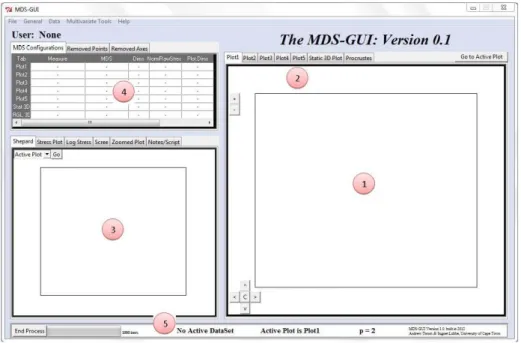
5.1.1 A Tour . . . 100
5.2 Multidimensional Scaling Capabilities . . . 102
5.3 Menu Structures of the Software . . . 102
5.3.1 Top Menu . . . 102
5.3.1.1 File Menu . . . 103
5.3.1.2 General Menu . . . 103
5.3.1.3 Data Menu . . . 104
5.3.1.4 Multivariate Tools Menu . . . 106
5.3.1.5 Help Menu . . . 108
5.3.2 Main Plot Menu . . . 110
5.3.3 Secondary Plot Menus . . . 111
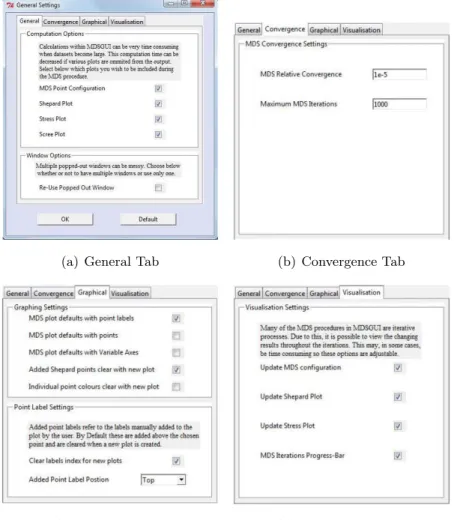
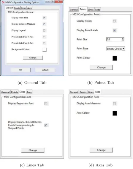
5.3.4 General Settings Menu . . . 111
5.3.4.1 General Tab (a) . . . 111
5.3.4.2 Convergence Tab (b) . . . 112
5.3.4.3 Graphical Tab (c) . . . 113
5.3.4.4 Visualisaiton Tab (d) . . . 113
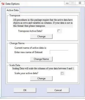
5.3.5 Data Options Menu . . . 113
5.3.6.1 Dimensions Tab . . . 114
5.3.6.2 Starting Configurations Tab . . . 115
5.3.6.3 Stress Tab . . . 116
5.3.7 Plot Option Menus . . . 116
5.3.7.1 General Tab . . . 116
5.3.7.2 Points Tab . . . 118
5.3.7.3 Lines Tab . . . 118
5.3.7.4 Axes Tab . . . 118
5.4 Overview of Features . . . 118
5.4.1 Plotting Tab Features . . . 119
5.4.2 p ≥2 . . . 120
5.4.2.1 Three Dimensions . . . 120
5.4.2.2 More Than Three Dimensions . . . 122
5.4.3 Shepard Plot . . . 123
5.4.3.1 Shepard Point Labeling . . . 124
5.4.3.2 Brushing the Shepard Plot . . . 125
5.4.4 Scree Plot . . . 128
5.4.5 Iterations Observable . . . 130
5.4.5.1 Stress Plots . . . 130
5.4.5.2 Progress Bar and End Process . . . 131
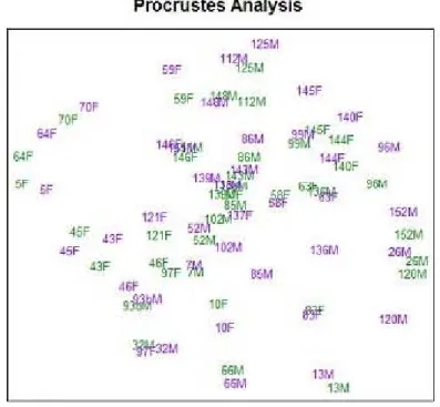
5.4.6 Procrustes Analysis . . . 132
5.4.7 Point Labeling . . . 133
5.4.8 Manual Alterations of Configurations . . . 135
5.4.9 Zoom . . . 137
5.4.10 Configuration Orientation . . . 138
5.4.11 Colour Options . . . 140
5.4.12 Variable Axes . . . 144
5.4.13 Removed Points and Axes . . . 145
5.4.14 Notes/Script . . . 147
5.4.15 Save and Load Workspace . . . 148
5.4.16 Export to PDF . . . 149
5.4.17 Print . . . 151
5.4.18 Supporting Plotting Features . . . 152
5.5.1 MDS-GUI Development . . . 153
5.5.2 Challenges . . . 154
5.6 The MDS-GUI: Version 2 . . . 154
5.7 Similar Software . . . 155
5.7.1 iMDS . . . 156
5.7.2 XGVis and GGVis . . . 156
5.8 The MDSGUI Package and Supporting Documentation . . . . 157
5.8.1 User Manual . . . 157
5.8.2 MDSGUI Package Reference Manual . . . 158
5.8.3 Vignette . . . 158
6 Application of the MDS-GUI 159 6.1 Morse-Code Data . . . 159
6.1.1 Morse-Code: General Analysis . . . 160
6.1.2 Morse-Code: Configuration Analysis . . . 163
6.2 SynTReN Microarray Data . . . 168
6.2.1 SynTReN Microarray: General Analysis . . . 170
6.2.2 SynTReN Microarray: Configuration Analysis . . . 173
6.3 Breakfast Cereal Data . . . 177
6.3.1 Cereal Data: General Analysis . . . 179
6.3.2 Cereal Data: Configuration Analysis . . . 183
7 Conclusions & Recommendations 188 7.1 Significance of Research and Development . . . 188
7.2 Concluding Remarks About Objectives . . . 189
7.3 Data Study Conclusions . . . 191
7.4 Recommendations . . . 192
A Data Sets A.1-1
A.1 Skulls Data . . . A.1-1 A.2 Morse-Code Data . . . A.2-1 A.3 Breakfast Cereal Data . . . A.3-1 A.4 SynTReN EColi Microarray Data . . . A.4-1
B Supporting Documentation B.1-1 B.1 Reference Manual . . . B.1-1 B.2 Users Manual . . . B.2-1 B.3 Vignette . . . B.3-1
2.1 Example of MDS Ordination Configuration . . . 10
2.2 Accuracy of Distance . . . 21
2.3 Scree Plot Example . . . 24
2.4 Scree Slope . . . 25
2.5 Shepard Diagram Examples . . . 28
2.6 Example of Shepard Plots With One Distorted Point . . . 29
2.7 Skull Data Example . . . 47
2.8 Skull Data With Coloured Categories . . . 49
2.9 Skull Data: Cluster . . . 50
2.10 Skull Data: Axes of Variation . . . 53
2.11 Skull Data: Procrustes Analysis Example . . . 55
3.1 Non-Metric MDS: Transformation of Distances . . . 69
3.2 Majorising Algorithm Example . . . 74
5.1 The MDS-GUI . . . 101
5.2 The File Top-Menu . . . 103
5.3 The General Top-Menus . . . 104
5.4 Appearance Settings . . . 104
5.5 The Data Top-Menus . . . 105
5.6 Uploaded Data Menu . . . 106
5.7 The Multivariate Tools Top-Menus . . . 107
5.8 The Help Top-Menu . . . 108
5.9 Function Help . . . 109
5.10 About: Text Box . . . 110
5.11 Main Plot Options Menu . . . 110
5.12 Secondary Plot Options Menu . . . 111
5.13 General Settings Menu . . . 112
5.14 Data Options Menu . . . 114
5.15 MDS Options Menu . . . 115
5.16 p=1 Warning . . . 116
5.17 Plot Options Menu . . . 117
5.18 Configuration Table . . . 119
5.19 Three Dimensions Options . . . 120
5.20 3D Plotting . . . 121
5.21 Large Dimensions Options . . . 123
5.22 Matrix Editor . . . 124
5.23 MDS-GUI: Displaying Shepard Plot . . . 125
5.24 Labeled Shepard Points . . . 126
5.25 MDS-GUI: Specific Shepard Point Label . . . 127
5.26 Shepard Point Brushing . . . 127
5.27 Scree Plot . . . 129
5.28 Stress Plots . . . 132
5.29 Progress Bar and End Process Button . . . 133
5.30 Procrustes Analysis Example . . . 134
5.31 Label Point with Cursor . . . 135
5.32 Label Specific Point . . . 135
5.33 Moving Configuration Points . . . 137
5.34 Manual Zoom Controls . . . 138
5.35 Zoom Options . . . 139
5.36 Configuration Orientation Controls . . . 140
5.37 Configuration Orientation Changes . . . 141
5.38 Colour Categories . . . 142
5.39 Colour Tools . . . 143
5.40 Change Point Colour . . . 144
5.41 Display Variable Axes . . . 146
5.42 Variable Axes Removal . . . 146
5.43 Removed Item Tables . . . 147
5.44 Notes-Script Tab . . . 148
5.46 PDF Output: Plot1-Page1 . . . 150
5.47 PDF Output: Plot1-Page2 . . . 151
5.48 Popped-Out Plot . . . 152
6.1 Morse-Code Data: Best Results . . . 162
6.2 Morse Code: Procrustes Analysis . . . 163
6.3 Morse-Code Data: Diagnostic Plots . . . 164
6.4 Morse Code: Symbol Categories . . . 165
6.5 Morse Code: Length Categories . . . 166
6.6 Morse-Code Data: Labeled Points . . . 167
6.7 True Gene Association Network . . . 170
6.8 MicArray: Procrustes Analysis . . . 172
6.9 MicArray: Metric SMACOF (City-Block Metric) . . . 173
6.10 MicArray: Diagnostic Plots . . . 174
6.11 MicArray: Metric SMACOF with Coloured Groups . . . 175
6.12 MicArray: Deviating Pairs . . . 177
6.13 MicArray: p=3 Configuration . . . 178
6.14 MicArray: p=3 Shepard Plot . . . 179
6.15 Cereal Data: Shepard Plot Comparison . . . 181
6.16 Cereal Data: Kruskal’s Analysis Scree Plot . . . 182
6.17 Cereal Data: Kruskal’s Analysis Configuration . . . 183
6.18 Cereal Data: Kruskal’s Analysis Configuration (Axes) . . . . 184
6.19 Cereal Data: Kruskal’s Analysis Configuration (Shelf Axes) . 186 6.20 Cereal Data: Furthest Points . . . 187
2.1 Distance Matrix Example . . . 9
2.2 Coordinate Vectors: p = 2 . . . 9
2.3 Interpretation of STRESS-1 . . . 19
2.4 Binary Data Similarity Coefficient Key . . . 39
6.1 MDS Stress Values on Morse Code Data . . . 160
6.2 NRS Values on Microarray Data . . . 170
6.3 Stress-2 Values on Cereal Data . . . 180
A.1 Skull Variables . . . A.1-2 A.2 Skulls Data . . . A.1-2 A.3 Morse Code Symbols . . . A.2-1 A.4 Asymmetric Morse-Code Data . . . A.2-2 A.5 Symmetric Morse-Code Data . . . A.2-4 A.6 Kellogg’s Breakfast Cereal . . . A.3-1 A.7 Breakfast Cereal Variables . . . A.3-2 A.8 Kellog’s Cereal Data . . . A.3-2 A.9 Microarray Ecoli Genes . . . A.4-1
Introduction
1.1
Introduction
The use of statistical methods in the field of data analysis has expanded beyond being strictly performed by statisticians. Areas of research, in-cluding Biology, Sociology, Psychology, Marketing, Genealogy and Ecology, among others, are making increasing use of advanced statistical computa-tional methods in their research. With this ever growing demand for these procedures comes the necessity for statisticians to produce means of provid-ing these researchers with the ability to undertake such endeavors. Statis-tical programming languages, such asR and Stata, and more commercially, theSAS software and STATISTICA, are available to statisticians and non-statisticians alike. These programs however require a certain amount of prior statistical knowledge and have a steep learning curve. This is something that many non-statisticians may find intimidating.
An emerging niche among statistical programmers has become prevalent over recent years, and this is in the development of Graphical User Interfaces (GUIs) that allow for easy implementation of specific complicated statistical functions. The subject of this dissertation is based on Multidimensional Scaling (MDS) and the development of the MDS-GUI, which stands for the Multidimensional Scaling Graphical User Interface. This piece of software is designed for theR programming language and supplies the user with an interface that is easily navigable and is capable of performing and analysing
multiple methods of MDS.
1.2
Background Information
These statistical GUIs are developed with the primary intention of ease of use and interactability. As such, the programs are usually designed such that they are navigated and utilised in a point and click manner. The key benefit of such programs is that the coding aspect is removed from the process and they are therefore accessible by those who are either incapable of such com-puter programming, or not knowledgeable enough about the statistics of the functions to perform the task themselves. This trend of GUI development is particularly prevalent within the R programming community, with such examples as the BiplotGUI (la Grange et al., 2009) and the caGUI (Markos, 2010) which were designed to simply and efficiently perform biplot and cor-respondence analysis functions respectively. R is a convenient environment in which to create these types of software as it is free to all users and driven by user contribution of packages. A number of these packages are geared to aid with GUI development, such as the tcltk package (R Development Core Team, 2012) which providesR functionality of the tcltk development language. A notable gap in theRdatabase was found to be that there was a lack of GUI for performing Multidimensional Scaling techniques, which are highly useful in multivariate data analysis. This provided the opportunity to develop a suitable and interactive piece of software that provided all R users with the ability to perform MDS operations easily and without having to undertake the coding themselves.
The ordination methods of Multidimensional Scaling have been studied and used for decades and numerous works have been written on the sub-ject. The two primary sources of information for the MDS topics covered in this dissertation were Multidimensional Scaling: Second Edition (Cox and Cox, 2001) andModern Multidimensional Scaling Theory and Applications: Second Edition (Borg and Groenen, 2005).
1.3
Objectives
The objectives of the dissertation are related to both investigating MDS techniques and development of the MDS software. These objectives are summarised by the following:
1. Provide suitable information regarding Multidimensional Scaling and its methods in the context of the MDS-GUI. This includes full theoret-ical and mathemattheoret-ical explanations of the MDS algorithms, diagnostic tools and interpretation of its results.
2. Provide Information regarding the programming languages and pack-ages used in the development of the MDS-GUI.
3. Develop a fully functional version of the MDS-GUI. The software, upon completion, will become available for download from the relevant R websites.
4. Describe the MDS-GUI in full, including all components of the inter-face and complete discussion of its functionality.
5. Simultaneously demonstrate the results of the MDS-GUI and provide examples of interpretation of MDS based results.
1.4
Scope and Limitations
Multidimensional Scaling contains a broad number of topics and procedural aspects. The concepts behind many of these components of MDS theory are themselves vast and have been considered as research topics alone. As a result, most of these will not be investigated and will be taken as given during the presentation of theoretical concepts. An example of one such aspect which will not be investigated is the optimisation methods used in finding optimal results. Another feature of MDS is the vast number of methods that fall under the MDS category. The MDS-GUI only incorporates a subset of these, meaning that some MDS methods will not be featured in either the software or the documentation. The MDS-GUI will provide means of performing Classical Scaling, Least Squares Scaling, Metric and Non-Metric
SMACOF, Kruskal’s Analysis and Sammon Mapping. The statistical scope of the dissertation includes these six methods.
The scope, from a coding point of view, specifically involves the devel-opment of an interface for performing MDS procedures. The backing code however made use of preexisting code written to retrieve MDS results. This code was supplied by associated contributors and existingR packages.
This document, although addressing the development of the MDS-GUI to great extent, will not provide anyR ortcltk code during the discussions. Accompanying the document will be a disk containing all pieces of code related to the MDS-GUI (and the GUI itself). Interested readers are invited to look at this code for a better idea of the coding processes involved in the GUI functions.
1.5
Layout of Document
The layout of the remainder of this dissertation aims to first provide suffi-cient information regarding Multidimensional Scaling and then discuss the MDS-GUI itself. The remaining six chapters will cover the following.
Chapter 2 provides information regarding the theoretical concepts of Multidimensional Scaling. The Chapter discusses MDS and its results in general terms and without making too much distinction between the var-ious methods of MDS. This discussion includes an analysis of the MDS algorithm, stress and what a researcher is required to do to perform MDS when analysing their data.
Chapter 3 is focused on the mathematics of MDS. This includes descrip-tions of Metric and Non-Metric methods, isotonic regression, the SMACOF algorithm and the six MDS methods incorporated into the MDS-GUI.
Chapter 4 discusses the technical computer related aspects of the project. It provides information on all coding languages and packages that are utilised throughout the development of the MDS-GUI software.
Chapter 5 introduces the MDS-GUI and describes it in detail. The Chapter firstly gives a tour of the interface by describing each of the areas of the front-end of the software and the menus that control it. Following this, detailed descriptions and demonstrations of all the major functions of
the MDS-GUI are given. The Chapter ends off with short sections on the challenges of development, similar software and theMDSGUIR package.
The MDS-GUI is then put to use in Chapter 6, where its features and output are demonstrated with the use of three different sets of data. These data sets were selected to highlight the varying features that are applicable to different types of data. Interpretations of the results from a statistical point of view are also provided.
The document ends with Chapter 7, giving the conclusions and recom-mendations that were accumulated throughout the study and development process.
1.6
Notation
For convenience of the reader, the notation used throughout the document will be summarised here. Each example will be introduced in detail in the text. This Section simply provides a means of reference. In general, all matrices are referenced by an upper case boldface letter and elements of the matrix by the appropriate lower case letter.
• n: Number of objects/subjects in the data. • m: Number of variables of the data. • p: number of MDS plotting dimensions.
• Z: Data matrix in the form objects×variables, i.e. with dimensions
n×m.
• ∆: Symmetric dissimilarity matrix of objects. Dimensions are n×n. • δij: Observed dissimilarity between theith andjth objects.
• S: Similarity matrix of objects. Dimensions aren×n. • sij: Observed similarity been the ith and jth objects.
• X: MDS Coordinate matrix. Dimensions aren×p.
• D: Symmetric Matrix of Euclidean distances between points in X. • dij: Euclidean distance between the ith and jth objects inX.
• D: Matrix of disparities. Derived from admissible transformation ofˆ proximities.
• dˆij: Disparity between the ith and jth object.
The following convention will be followed with respect to programming languages,R packages and functions.
• Programming languages will be italisised, e.g. R. • R packages will be in boldface, e.g. MASS.
The Theory of
Multidimensional Scaling
This Chapter serves to inform the reader on the theoretical concepts of Mul-tidimensional Scaling with a focus more on the procedural aspects of the topic rather than the in-depth Matrix Algebra. This Mathematical theory will be covered in the following Chapter The Mathematics of Multidimen-sional Scaling.
The content of the Chapter will include the theory of MDS as a process. It will also describe the diagnostic tools used to analyze the performance of the methods, as well as the place that Multidimensional Scaling holds in practical data analysis.
2.1
An Introduction to Ordination
Ordination is a general term for techniques in multivariate analysis which adapts sizable matrices of data in such a way that when projected onto a space of fewer dimensions, intrinsic patterns within the data may be vi-sually inspected (Clark, 2005). There are a number of ordination methods that have been developed, including: Factor Analysis, Correspondence Anal-ysis, and Principle Component Analysis. The subject of this dissertation, however, is the group of ordination methods collectively known as Multidi-mensional Scaling. Some texts refer to MultidiMultidi-mensional Scaling as
pal Coordinate Analysis, however a more accurate description would be that Principal Coordinate Analysis is an alternative name to what is called “Clas-sical Scaling”, which is only one of the many forms of MDS. Each of these methods of ordination, while conceptually producing similar visual outputs, are vastly different and have their own specific uses. A more detailed view on the primary similarities and differences between Multidimensional Scal-ing and the other methods of ordination can be found in Section 2.12 of this Chapter under the headingMultivariate Methods Related to MDS.
2.2
Multidimensional Scaling
Like all ordination methods, the purpose of all the types of MDS is to provide a visual representation of a large data matrix in a low dimensional space. From a simplified point of view, MDS is used to provide a mapped, usually two or three dimensional, approximation of the patten of proximities found in a given set of data. This set of proximities is either in the form of dissimilarities or similarities between objects in the data.
More technically, what Multidimensional Scaling does is find a set of vectors inp dimensional space (wherep has been predefined) such that the matrix of Euclidean distances among them corresponds as closely as possible to some function of the input matrix according to a certain criterion, most commonly Stress. Stress and the other criterion measures for goodness-of-fit will be analysed later in this Chapter in Section 2.4 under the heading Stress & Strain. Each vector is then treated as the set of coordinates of the corresponding dimension, thus allowing a visualisation inp dimensional space such that each object in the data is represented by a point on the plot. The distances between these plotted points represents, as accurately as possible, the original similarities (or dissimilarities) of the data. This im-plies that similar pairs of objects are represented by points that have been positioned closer to one another and dissimilar objects are represented by points that have been positioned further apart from each other. It is for this reason that Mair and de Leeuw (2008) describe MDS as a set of methods for discovering “hidden structures in multidimensional data”. As the procedure only tries to match the mapped, Euclidean distances, as closely as possible
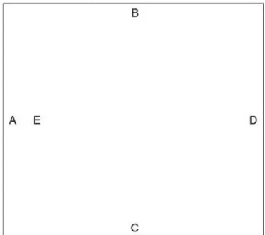
to the matrix of proximities, it is not so much an exact procedure as rather a way to rearrange the points (objects) in an efficient manner so as to arrive at the configuration that best approximates the observed distances. The fol-lowing example is trivial, and merely serves to demonstrate the relationship between proximity data and visual mapping. Table 2.1 demonstrates the distances, measured with an Euclidean metric, between five points. These points have been labeled fromA, B, C, D, E. Since the proximities in this case are specifically distance based, the proximity type is clearly dissimilar-ity. A Classical Scaling procedure withp equal to two, when performed with this data as an input, produces the graphical results shown in Figure 2.1 with corresponding vectors in Table 2.2.
Table 2.1: Distance Matrix Example
A B C D E A 0 3 3 4.24 0.5 B 3 0 4.24 3 2.77 C 3 4.24 0 3 2.77 D 4.24 3 3 0 3.74 E 0.5 2.77 2.77 3.74 0
Table 2.2: Coordinate Vectors: p = 2
V1 V2 A -1.802 0.000 B 0.346 2.120 C 0.346 -2.120 D 2.429 0.000 E -1.285 0.011
Figure 2.1: Example of MDS Ordination Configuration
points A, B, C, D. The fifth object E, is shown to be a point within the square with a strong relationship to objectA. This example is unfortunately unrealistic in that the MDS representation of the proximities is just about perfect. Real applications are expected to have a certain amount of distor-tion in their results. It should be noted that the plot itself has an aspect ratio of one. A square grid is very important when producing MDS results as it preserves equality in the ratio of distances over the plotting dimensions. It is the norm that thep-dimensional space onto which these points are mapped is Euclidean. While this is not theoretically a requirement, it is the only logical way of portraying the solutions as MDS aims to take compli-cated information and portray it in a format accessible to a human observer. The proximity matrix however is often found to be calculated using distance measures other than Euclidean. A comprehensive list of methods for dis-tance measurement is provided and discussed in Section 2.8. The number of dimensions onto which the points are mapped is also typically either one, two or three as these are the only options for producing visual images com-prehensible to the human brain. The MDS procedures are, however, in no way limited in terms ofp. The number of dimensions that are used in the
B
A
E
o
procedure allow us to explain proximities of the data in that number of dimensions. In an example of distances between cities, one could explain distances in terms of two dimensions, being north/south and west/east. Al-ternatively a further dimension could be included which could account for the altitude of the cities.
While there are a wide range of types of Multidimensional Scaling, there are two categories under which the various methods fall. These two cate-gories are Metric and Non-Metric Multidimensional Scaling, both of which will be discussed in brief detail here.
2.2.1 Metric Multidimensional Scaling
The techniques of Metric Multidimensional Scaling are structured in such a way that there is an assumption of metric qualities in the measurement of the proximities. That is to say that the extent of the (dis)similarities between points are taken into account. Thus the distances in metric MDS space preserve the intervals and ratios as well as possible (Wickelmaier, 2003). The use of Metric Multidimensional Scaling is only valid when the assumption of metric distances can be justified. Methods that fall under Metric Multidimensional Scaling include: Classical Scaling (Principal Coor-dinate Analysis), Least Squares Scaling and Metric SMACOF. All Metric MDS methods are discussed in detail in Section 3.2.
2.2.2 Non-Metric Multidimensional Scaling
In many situations the metric assumptions described above are too strong for the data at hand. It is under these circumstances that the use of Non-Metric Multidimensional Scaling techniques may be more appropriate. Under the theories of non-metric multidimensional scaling the extent of the proximities is irrelevant. Only the ordering of the (dis)similarities is factored during the derivation of the MDS configuration. Methods that fall under Non-Metric Multidimensional Scaling include: Kruskal’s MDS, Non-Metric SMACOF and Sammon Mapping. All Non-Metric MDS methods are discussed in detail in Section 3.3.
2.3
The General MDS Algorithm
Within Multidimensional Scaling there are a number of different subsets of MDS techniques, most with a classification of either metric or non-metric. A number of these methods will be described and investigated in detail in Chapter 3 The Mathematics of Multidimensional Scaling. The majority of the methods, however, follow the same general algorithm in terms of how the procedure progresses and at what point it terminates. This basic algorithm is described below.
The process of Multidimensional Scaling may begin in one of two ways. The first of these is with a data matrix Z, consisting of n rows of samples andm columns of variables. The n ×n proximity matrix used in the MDS process is derived from this data matrix. As mentioned before, this proxim-ity matrix can be in the form of dissimilarities,∆, or similarities,S, between the samples. Alternatively, the n × n proximity matrix is provided inde-pendently and in this case, no proximity calculation is required. A typical method of dissimilarity calculation is using an Euclidean measure to find the pairwise distances between samples. The matrix does not necessarily have to be symmetric as, depending on how the proximity values are calcu-lated, the differences between two objects might be different depending from which direction the measure was taken. For example, if elevation is being assessed the difference between two points would yield both a positive and negative value depending on the starting point. This proximity matrix is however required to be square and should, as best as possible, be complete. Once the proximity matrix has been derived the data collection is complete. Many MDS algorithms specifically require the dissimilarity matrix, ∆, as input. In this case similarities are simply transformed to dissimilarities. The elements of the dissimilarity matrix are δr s and refer to the original
mea-sured proximity between therth and sth objects. Some MDS methods and
programs make allowances for asymmetry in their proximity data. The soft-ware discussed in this dissertation, however, strictly requires all proximities to be symmetric. The following criteria therefore must hold.
δij = 0 if f i=j
δij +δjk ≤δik ∀i, j, k
Before the MDS procedure commences, the desired number of dimensions must be chosen for the ordination. Further in this Chapter the concept of Scree Plots will be discussed. These plots aid the researcher in determining the most appropriate number of p dimensions that should be used for the particular data. However, for all intents and purposes of describing this simple algorithm, the specific number of dimensions being used is irrele-vant so no further detail on the dimensionality of the ordination need be given at this point. With the proximity matrix calculated and p, the num-ber of dimensions, decided upon, the Multidimensional Scaling procedure may commence. The process begins with an initial configuration of points in the p dimensional space, with each point representing an object from the data. This configuration, described by the coordinate matrix X with dimensions n×p, can be entirely random or else could be based on some other prior knowledge, such as the results of some other ordination, or a pattern suspected by the researcher. It should be noted however that due to the problem of local minima, the initial configuration may influence the final result. This problem of local minima will be discussed in Section 2.13. The distances between points in the configuration are then calculated. This calculation is almost exclusively done using an Euclidean Metric as the plot-ting plane that is observed by the researcher is Euclidean by nature. This symmetric matrix of ordination based distances has dimensions n×n and is referred to as D (dr s is the distance between the rth and sth objects
within the MDS configuration). In the cases of Non-Metric Scaling, these ordination based distances are then regressed against the original distance matrix∆using one of a number of regression methods, and are fitted using a method of least squares. The transformed distances are generally referred to as ˆddistances, and form part of the symmetricn×nmatrix ˆD. All fitted elements of ˆD are referred to as ˆdr s. Metric cases see the method of least
squares fitting simply the ordination distances and the proximities.
n−1 X i=1 n X j=i+1 (f(δij)−dij)2 = n−1 X i=1 n X j=i+1 ( ˆdij −dij)2 (2.1)
The sum of squares component in (2.1) is the basis of the function usually referred to as stress, which is an integral component of most Multidimen-sional Scaling techniques. Stress is the general term and actually comes in a number of different forms, the most important of which are described in the following Section. The common interpretation of stress is however, that the smaller the stress the better the fit, as there is a smaller (squared) dif-ference between the distances in the configuration of points and the original proximities.
With stress as an indicator of goodness-of-fit of a configuration, the MDS process begins to move the points of the configuration. The nature of how the points are moved is dependent on the method of MDS being used. Af-ter each adjustment, the matrix of ordination distances, D, is calculated (and in Non-Metric cases, so is ˆD) and subsequently so is the stress of the configuration. If a new configuration yields a stress value greater than the configuration before it, it is discarded. Alternatively, when a new config-uration yields a smaller stress value than before, the old configconfig-uration is discarded and the new configuration becomes active. Many formats of MDS have only monotonically decreasing stress, meaning that any stress value will only ever be smaller than or equal to its preceding value. The configuration is thus improved by moving the points of the ordination in small amounts in the direction that causes the stress to decrease most rapidly. This procedure is then continued until either the stress has reached a value small enough to satisfy the researcher (a certain threshold value has been achieved) or a point of convergence has been reached. Convergence is reached when the difference in stress between two consecutive configurations is smaller than a certain tolerance that has been predefined. This implies that a larger pre-defined tolerance will usually cause convergence sooner than when a smaller tolerance is used. None the less, this point of convergence indicates that the accuracy of the configuration is unable to improve and thus a minimum stress value (local or global) has been met.
At this point the procedure has stopped. In the event that convergence occurs at a point where stress is considered unacceptably high, the researcher must make the choice of either making adjustments to the setup of the proce-dure (starting configuration, tolerance, etc.) or abandoning MDS in favour
of a more appropriate method of ordination for their specific needs. Another option that may be available is to increasep, the number of dimensions of the ordination configuration. As will be explained in Section 2.5, increasing p will always decrease the final stress value and thus demonstrate a bet-ter fit. On the other hand, in the event that the process stopped due to stress reaching an acceptably low value, the researcher is likely to be satis-fied with the outcome of the MDS procedure. The resulting configuration, with coordinates X, will thus display the arrangement of the points that best represents the proximity matrix in the chosen p dimensions. The ac-tual orientation of the axes in this final configuration solution is arbitrary. The decision of how the ordination should be oriented is usually a subjec-tive decision of the researcher, who is likely to make a decision based on what is considered the most easily interpretable orientation. For example, North-South is likely to be appropriate as the vertical on a two dimensional geographical point map. The rotation of the configuration is irrelevant in the context of MDS since distance is indifferent under rotation. The MDS result is thus unlikely to have North-South on the vertical, which leaves the final rotation at liberty of the researcher.
The above procedure can be summarized in the following steps.
1. Assign objects to points in initial configuration in the p dimensional space. Then ×p coordinate matrix is referred to as X.
2. Compute distances among all pairs of points in configuration to form a matrix of distances,D.
3. When performing Metric MDS, do 3(a). When performing Non-Metric MDS, do 3(b).
(a) The D matrix is then compared to the original matrix of prox-imities,∆. Stress is then calculated.
(b) TheD matrix is then compared to ˆD, the fitted values resulting from some function of∆. Stress is then calculated.
4. The coordinates,X, are adjusted in such a way that stress is improved upon from the previous configuration.
5. Steps two to four are repeated until either:
(a) Stress has reached an acceptably low point, or
(b) The value of stress has converged given the set tolerance. (c) The value of stress has not converged given the set tolerance, but
the maximum number of iterations have been reached
In the case of 5(b) or (c) where stress is unacceptably high, do 6.
6. Perform one or more of the following.
(a) Tolerance value decreased. (b) Starting configuration altered.
(c) p is increased.
(d) Or alternatively, MDS is abandoned.
2.4
Stress & Strain
The previous Section made extensive reference to the functions collectively known as “stress” in the computation procedure during the Multidimen-sional Scaling algorithm. While there do exist other measures to evaluate the degree of correspondence between the distance among points implied by the MDS map and the observed proximity matrix, the various forms of stress have become the norm within Multidimensional Scaling.
2.4.1 General Form of Stress
The general form of the various stress functions is as follows:
v u u u t nP−1 i=1 n P j=i+1 (f(δij)−dij)2 scale (2.2)
In the equationδij refers to theijthelement of then ×nobserved proximity
Cox, 2001). The dij, as described, are the elements of the square matrix,
D, of distances between points across all dimensions in the resulting MDS configuration. D is assumed to be symmetric, thus dij = dji, dii = 0,
i= 1, ..., n−1 andj=i+ 1, ..., n. Finally, the ‘scale’ component refers to a
constant scaling factor, used to keep the value of stress within the convenient range of between 0 and 1. Stress therefore acts as an inverse measure of the goodness-of-fit of an MDS configuration, as stress closer to 0 indicates a good fit (with stress of zero indicating a perfect mapping of the points) and stress values closer to 1 indicating a very poor fit.
The transformations of the input valuesf(δij) used depends on the type
of MDS that is being used to perform the operation. Some appropriate and relevant transformations will be observed and discussed in both Section 2.7, the Data Section of this Chapter, and throughout Chapter 3, but briefly the two major cases will be mentioned here. In metric scaling f(δij) = δij
(the identity transformation), which means that the raw input proximity data is compared directly to the mapped distances. In non-metric scaling however,f(δij) is usually in the form of a monotonic transformation of the
MDS proximities, and is used to minimise the stress function.
The general form of the stress equation, is given by (2.2). The three most common forms of stress will now be discussed, these being: STRESS-1 (or Kruskal’s Stress); STRESS-2; and Normalized Raw Stress.
2.4.2 STRESS-1
The most common form of stress, at least within non-metric MDS, was developed by (Kruskal, 1964) and is known as Kruskal’s Stress, or more commonly, STRESS-1. Throughout this dissertation it will be referred to exclusively as STRESS-1. In this version of stress, the scaling factor is
P P
di2j which is the sum of squared distances between all pairs of points
comprising the MDS mapped configuration of points. The resulting com-plete formula for STRESS-1 is:
ST RESS1 = v u u u u u u t nP−1 i=1 n P j=i+1 (f(δij)−dij)2 nP−1 i=1 n P j=i+1 di2j (2.3) 2.4.3 STRESS-2
STRESS-2 is an alternative to STRESS-1 and differs only with regards to the scaling factor in its calculation. The scaling factor becomesP P(dij−d..)2
whered..is the overall mean distance of all pairs of points combined in the ordination configuration. The equation 2.3 shows the complete formula for STRESS-2. ST RESS2 = v u u u u u u t nP−1 i=1 n P j=i+1 (f(δij)−dij)2 nP−1 i=1 n P j=i+1 (dij −d..)2 (2.4)
The scaling factor of STRESS-2 places more of a restriction on the con-figuration and results in higher stress values (Cox and Cox, 2001) and for this reason is often considered less desirable than STRESS-1.
2.4.4 Normalised Raw Stress
Normalised Raw Stress (NRS) is another form of Stress that is widely used. It is defined as the squared version of STRESS-1 and thus has the following formula: N RS= nP−1 i=1 n P j=i+1 (f(δij)−dij)2 nP−1 i=1 n P j=i+1 d2 ij (2.5)
The effect of squaring the STRESS-1 value results in normalised raw stress scores being much lower than those of STRESS-1. This version of stress can thus be considered to be less strict than others.
2.4.5 Strain
STRAIN is a loss function that is specifically applicable to Classical Scaling. While the stress values already discussed may be used on Classical Scaling examples with the same interpretation as other MDS methods, the option of Strain is also applicable. The STRAIN formula is given by equation (2.6), where then ×m data matrix is given byZ and the matrix of MDS configuration coordinates is given byX.
ST RAIN =tr[(ZZT −XXT)T(ZZT −XXT)] (2.6)
2.4.6 Interpretation of Stress
As stated, a stress value of zero indicates a perfect fit of points from the MDS procedure; however it is not necessary for an MDS based mapping to have zero stress in order to be informative or useful. Stress values close to zero are also tolerable due to an allowable amount of distortion in the model. The cut off value for what range of stress is permissible is largely subjective and may vary depending on the type of data being used or the level of accuracy desired by the researcher. It is also important to note that stress is expected to be higher on data with more samples and more variables, so extreme care must be taken when comparing stress values of data sets with different sizes. There are however, a few broad rules of thumb which may be useful for researchers to remember when performing this method of ordination. The following table summarizes the suggested rules when using STRESS-1.
Table 2.3: Interpretation of STRESS-1
Interpretation Stress Value
Ideal 0 - 0.1
Acceptable 0.1 - 0.15 Unacceptable 0.15 - 1
acceptable, a certain amount of care must be exercised when interpreting the configuration of points. By definition, any amount of stress that is present is due to at least one of the distances between a pair of points being distorted on the MDS configuration (possibly all to some degree). This means that whenever one wishes to make certain conclusions based on specific pairings, it is wise to first check on the accuracy of that specific element of the configuration. Necessary diagnostic tools do exist for this type of checking, and will be elaborated on in Section 2.6. On the other hand, in general, even mappings with higher stress values are potentially able to provide some sense of what small scale patterns exist within the data. That is to say, only patterns when viewing the configuration from a zoomed out perspective might be reliable. Zoomed in observations of intricate details (large scale patterns) would not be reliable. This is due to the fact that longer distances tend to be more accurate than shorter distances on a relative scale. This claim can be verified with the aid of a simple example.
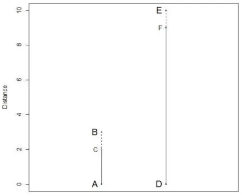
Figure 2.2 demonstrates how longer distances are generally more accu-rate. In the figure we see the lengths between two different point pairings. These pairings are A-B and D-E with the true distances between points seen to be 3 units and 10 units respectively. The distances between points A-C and D-F however represent the lengths between the original points as seen from an MDS ordination configuration. The MDS calculated lengths for the pairings are 2 and 9 units respectively. In both cases, therefore, the ordination distance is exactly 1 unit short of the true distance. It is simple then to see that in the case of this ordination result, A to C is 66% accurate of A-B while D to F is 90% accurate of D-E. The greater distance therefore exhibits greater accuracy than the shorter when faced with the exact same error.
Using Normalised Stress (NRS) as an example, the effect on the two scenarios is N RSAB(C) = (3−2)2 22 = 0.25 and N RSDE(F)= (10−9)2 92 = 0.012
Figure 2.2: Accuracy of Distance
though the deviation is one unit in both cases.
2.5
Dimensionality
The process of Multidimensional Scaling requires a choice of the number of p dimensions in which the configuration of points is to be mapped. As mentioned before, in the event that an MDS procedure results in a final stress value that is unacceptably high, one option available to the researcher is for the procedure to be performed again with a change in output dimension. At this point, it should once again be noted that while in practice the only dimensions that can be visually illustrated and analysed are dimensions one, two and three, MDS is not limited to these. In fact the procedure is able to allocate a configuration of points up ton−1 dimensions; wheren is the
o F 00 00
•
u C ~"
~ B N C oA
Dnumber of objects/samples in the data set.
When observing stress values for different dimensions usually suggests that as the number of dimensions is increased, the stress value will decrease. Consider a solutionX:n×hand the dimensions is then increased top > h. All MDS solutions are based on some form of optimisation. If the solution X : n×p has a larger stress than X : n×h, the optimal solution in p dimensions would beX:n×p= [X:n×h 0 :n×(p−h)] which shows that the stress of the optimal solution will be at least the same as the h-dimensional solution, and possibly smaller. In general, the value of stress will decrease at a decreasing rate as the number of dimensions is increased untilp reaches a certain value.
While the above statement is true (increasing dimensions enough is guar-anteed to drop stress), realistically stress is likely to be caused, to some extent, by random measurement error. An example illustrating this may be where a researcher is interested in the distances between the tops of buildings that are measured in a hypothetical city center. In this case, it is obvious that the true number of dimensions is three for this set of data (latitude, longitude and altitude) so theoretically a three dimensional MDS configuration should have zero stress. Realistically however, it is most likely that there will be some small amount of stress, which will be due entirely to measurement error. In cases such as these, where the precise number of dimensions is known and applied in the configuration, the value of stress can be used as a direct measure of the accuracy of the data. In this scenario, increasing the number of dimensions will eliminate this stress, in which case the excess dimensions of the MDS configuration will be describing the error of the measurement. Unfortunately, it is very seldom that the case be as clear cut and easily interpretable as this, so such convenient observations are not always possible.
There are two major issues with increasing the number of dimensions in such an ordination procedure. The first problem is obviously that the higher the dimension, the more difficult the interpretation. The most obvi-ous drawback is that any dimension over 3 cannot be graphically portrayed which means that the element of being able to quickly analyse a plot for pat-terns and groupings be eliminated. The second issue with a large number of
dimensions is that with every increment of dimension additional parameters are to be taken into account estimated from the raw data. In the event that sayn−1 dimensions are used, the complexity of the outcome is for all intents and purposes as complex as the data itself. Having said this, there do exist applications of MDS in which a high number of dimensions is not a problem.
Solutions of Classical Scaling (Principal Coordinate Analysis) are nested, regardless of the p used. That is,X:n×p= [X:n×h X∗]. This means
that the firsthcoordinate vectors will always be the same no matter what the adjustablep is. Most other MDS methods, which are based on optimisation, are not nested. Therefore, asp changes, the firsth dimensions also change.
2.5.1 Euclidean Embedding and Dimensions
As previously described, a number of cases exist which have an effect on the dimensionality of an MDS procedure. The following three cases are defined when the data space is Euclidean and therefore the matrix D is comprised of Euclidean distances.
The first of these cases is when the distance metric used is itself Eu-clidean. In this scenario, when p = m, the value of stress will be zero. The second case is when the distance calculation is Euclidean Embeddable. This means that despite having definitions different to a Euclidean Distance the distance information is still preserved when depicted in a Euclidean space. In this event, when p = n−1, the value of stress will be zero. The final case is when the distance calculation is Non-Euclidean Embeddable. These cases will never achieve a stress value of zero regardless of the value of p.
2.6
Diagnostic Tools
Multidimensional Scaling is a multivariate tool that, by its very nature, will produce results with an expected amount of distortion or error. It is important for a researcher undertaking tasks by using Multidimensional Scaling to understand the distortion of their output in order to improve on the results. A number of diagnostic tools exist and are used for analyzing
the output of Multidimensional Scaling Procedures, some of which will be discussed in this Section.
2.6.1 Scree Plot
Figure 2.3: Scree Plot Example
The problem of deciding on the number of dimensions to specify for a Multidimensional Scaling procedure on a given set of data can be made easier with the use of a Scree Plot. A Scree plot is achieved by running MDS on the data a number of times,ceteras paribus, with only the number of output dimensions changing. The resulting stress value is recorded after each run. The Scree Plot thus portrays the curve of plotting stress versus dimension.
As stress has already been described to decrease as dimensions increases, the plot demonstrates a decreasing monotonic function. The appropriateness of the dimensionality of the data is revealed by the shape of the rate of decline of stress. Figure 2.3 shows an arbitrary example of a Scree Plot with an easily interpretable shape. The Scree Plot example shows an obvious kink in the curve, otherwise referred to as an “elbow” in the plot. It is at this point that an indication of the true dimensionality of the data is revealed.
·-
'"
'"
"
..
,
..
,
,
.
"
'"
..
••
••
Scree Plot
Strvss by ()m""'SIOl1"'
l,~::;-..,
..
,
•
This elbow is obviously the point where increasing the dimensions yields a diminishing return on the stress, and thus the most appropriate MDS model has as many dimensions as the number of dimensions at the elbow. Returning to the example of measuring the distances between building tops. If this study were to be performed, it is quite likely a resulting Scree Plot would look very much like the example shown in Figure 2.3. The example shows the value of stress dropping steeply from the first dimension until the third, and subsequently the curve flattens out. The ‘elbow’ of the curve very clearly occurs when p is three and thus, as expected, p = 3 is the most appropriate number of dimensions to use in the MDS procedure. As mentioned in the previous Section, it is highly likely that some element of measurement error occurs which are explained by all dimensions greater than 3. The stress values for all p > 3 in the Scree Plot allow for visual inspection of the nature of this stress due to measurement error.
Figure 2.4: Scree Slope
The derivation of the naming of the Scree Plot may be of interest to some readers. The word ‘scree’ is a geological term which refers to the build up of debris which collects at the lower part of a rocky slope. The resulting slope is called the ‘Scree Slope’. The image shown in Figure 2.4 gives an example of such a scree slope and provides some insight into why the Scree Plot has been aptly named.
The portion of the curve that occurs to the right hand side of the elbow is effectively the scree slope, and the ‘debris’ is made up of what has been called
factorial scree. This refers to the non systematic noise and measurement error that the further dimensions account for.
In reality, such clear elbow points in the scree plot are not always so ob-vious. This usually means that a certain amount of subjective interpretation is often required in interpreting such Scree Plots.
2.6.2 Shepard Plot
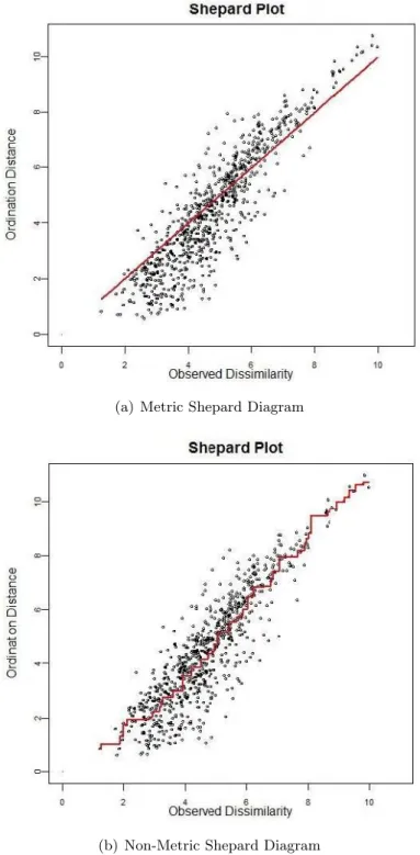
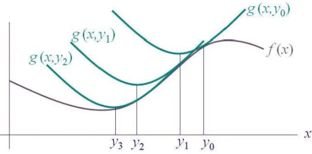
Another tool for judging the accuracy of an MDS procedure is the Shepard Diagram (Shepard, 1962). The diagram is a two dimensional scatter plot with the X-axis corresponding to the input proximities (δij) and the
Y-axis corresponding to both the MDS distances (dij) and the transformed
proximities ( ˆdij). Each point on the diagram represents a pairing of the
subjects in the data. This means that the Shepard diagram will have n2 points, wherenis the number of objects in the data. The Shepard diagram is therefore laid out in such a way that an observer is able to assess the accuracy of the ordination configuration with regards to every pairing individually. Since the observed distance will never change, each point will be isolated to a single vertical line, and therefore, the point will move up and down the line depending on the result of the ordination. Examples of the Shepard Plot are found in Figures 2.5(a) and 2.5(b). In both instances, the information is based on an MDS result where the data has 40 objects, and therefore 780 points.
The error of each point in the Shepard Diagram can be directly assessed by measuring the vertical distance between the actual location of the point and its hypothetically correct location. This hypothetically correct location depends on the type of MDS being performed. In metric MDS, where ob-served distances require matching, the distance between a pairing has been represented exactly when its X and Y coordinates are equal as the observed distance equals the ordination distance. Continuing this logic, a configura-tion that has a perfect fit will have all the points in a straight line along
y=x. Figure 2.5(a) is an example Shepard Plot from a metric MDS result. Included in the plot is a line through the diagonal, indicating the optimum fit. A configuration with a poor fit will have a Shepard Plot with points
de-viating far from this line. In Non-Metric MDS however, the relaxed metric assumption means that ordination distances do not strictly need to match the observed distances. Instead only the ordering of points is taken into account. In these non-metric instances the representation is exact when the observed distanced matches the transformed disparity ˆd. This means that on the Shepard Diagram it is the vertical distance been the point and the transformation curve that shows the amount of deviation in the represen-tation of the object pairing. Figure 2.5(b) shows a Non-Metric MDS based Shepard Diagram. The transformation curve in this case is a step function derived from an isotonic regression transformation.
The most useful element of the Shepard Diagram as a diagnostic tool is that, unlike evaluating a stress value, it is clear to see where the deviations in the predicted configurations lie. This allows the researcher to easily pick up on clear outliers and identify possible systematic deviations. It is also useful to note that the diagram shows the composition of the stress value. For metric MDS the sum of squared vertical distances between the points and the diagonal line forms the common component of most stress formulas. In non-metric cases, it is the sum of squared vertical distances between the points and their fitted values, represented by the transformation curve.
Figure 2.6 gives the example of how the Shepard Diagram can be used for such diagnostic purposes. Both plots show information on the exact same data as depicted in Figure 2.5(b) except in each scenario a single point has been positioned very inaccurately. Inspection of the Plot in 2.6(a) reveals exactly 39 points are positioned very obscurely and can certainly be seen to be well out of place. A researcher would confirm quickly that these points in fact relate to each of the 39 pairs that the single misplaced point has with the other objects and identify it to be a point of concern. The researcher would also be able to determine the nature of the inaccuracy. Since it is clear that for each of the 39 pairings of interest, the ordination distance is longer than the observed distance. This would imply the point is positioned outside the group and not incorrectly within it. If alternatively the point were to be severely misplaced within the group, a situation like that shown in Figure 2.6(b) would arise. This Shepard Diagram reveals a clear misplacement of points above and below the majority of points. The
(a) Metric Shepard Diagram
(b) Non-Metric Shepard Diagram
Figure 2.5: Shepard Diagram Examples
•
u C ~ 0 c 0 15 c ~ 0•
u C ~ o c o ro c ~ o•
,
•
,
Shepard Plot..
.
'.
.
'.
•
•
Observed Dissimilarity Shepard Plot•
•
•
Observed Dissimilarity(a) Out of Group Distortion
(b) In Group Distortion
Figure 2.6: Example of Shepard Plots With One Distorted Point
•
u C ~"
c 0 iii c l' a•
u C ~"
c o iii c 'E a,
,
•
•
~...
. .
....
...
~.
, '. Shepard Plot"
OLJ~IV~ Di~~illlil<llily Shepard Plot for Tab1.
.
' .',
,,
.
ObseJV€d Dissimilarity
..
points found below the others would show which pairings have been placed closer together than what would have been ideal. See also Section 5.4.3 for further illustration of interpretation of the Shepard Plot.
The visual look of the Shepard diagram is different depending on the type of data being used as well as the format of Multidimensional Scaling. The major variation in look of the diagram depends on the type of proximity matrix used. When the proximity matrix has information regarding the similarities between the items, the Shepard Plot will have a negative slope of points. The logic behind this is intuitive, since the X-Axis will represent the similarities of the data, and the Y-Axis remains representing distance between points in the ordination configuration. This implies that pairs that have a high similarity have a small ordination distance and pairs with low similarity will have longer ordination distances. Thus a negative slope. On the other hand, when proximities are dissimilarities the plot will have a positive slope. The logic to this is similar. The plot itself will also give an idea, to the trained eye, of the type of MDS that has been used. In metric scaling the line of points will be straight. In non metric scaling, however, the points will form a weakly monotonic function.
2.7
Data
Multidimensional Scaling is applicable to data in any of a number of forms. While some data sets are comprised ofn objects andm variables, other fac-tors do come into effect that may influence how MDS should be approached. For example, the formal definition of number of ‘modes’ and ‘ways’ of the data may alter the most appropriate form of MDS to be utilised. These and various data classifications and transformations will be discussed in this Section.
2.7.1 Types of Data
Several classifications of data exist that vary depending on how data is recorded and what it represents. Four major scale classifications of data have been identified and are listed below.
2.7.1.1 Nominal Scale
Data collected using the nominal scale represents only categorical informa-tion. If numbers are chosen to represent certain categories they will have no numerical interpretation. Letters are just as appropriate to represent the different classes.
2.7.1.2 Ordinal Scale
Ordinal data is data that can be ranked but does not hold any quantitative property. Recording the positional results of a race is an example of ordinal data. It can be observed that 1st place was faster than second, but no information regarding the extent of difference is given.
2.7.1.3 Interval Scale
Data collected on the interval scale is quantitative by nature and thus, unlike the previous two scales, exhibits continuous qualities. Therefore under the Interval scale, the difference between points is meaningful and the extent of the difference is recorded.
2.7.1.4 Ratio Scale
The final scale is the Ratio Scale, which has a continuous nature like the In-terval Scale, but also is defined by a relevant zero point. Variables measured on the Ratio Scale can therefore never be less than zero. For example tem-perature measure in degrees Celsius is not measured on the ratio scale since negative temperatures exist. Temperature measured in Kelvin however is on the ratio scale since zero Kelvin represents the lowest possible temperature.
2.7.2 Modes and Ways
The four scales determine how the data is measured, but do not necessarily describe the data as a whole. Two definitions that do make these general descriptions are termed ‘modes’ and ‘ways’. Modes are defined as the num-ber of sets of objects that occur within one data set. Cox and Cox (2001) uses the example of data being gathered from a number a judges tasting a
number of whiskies and comparing them to one another. In this scenario, the data would be two mode, with the judges and the whiskies being the two modes. The ways of a data set is defined by the number of indexes that exist between objects. In this whisky judging example, there are three ways, as the three index’s are the two whiskies being compared and the judge who compared them.
The most common form of proximity data used in Multidimensional Scaling is one mode and two way, i.e. the whisky example with only one judge.
2.7.3 Transformations of Data
Non-Metric Multidimensional Scaling is appropriate when only the rank ordering of the dissimilarities is relevant to the data. In these cases it is de-sirable to assign numerical values to the proximities in such a way that these values, the ˆddisparities, exhibit the same rank order as the data (Groenen and van de Velden, 2004). These methods of assigning appropriate ˆdvalues are the transformations of data relevant to MDS. Therefore, in Non-Metric MDS, the process is simultaneously required to obtain a configuration X and the corresponding ˆD matrix with each iteration. The transformation that will be used exclusively throughout this dissertation will be the isotonic regression transformation, sometimes referred to as monotone regression or ordinal transformation. This process will be described and illustrated in Section 3.3.
Other examples of transformations of the data to the ˆddisparities are (Borg and Groenen, 2005): the ratio transformation, the interval transfor-mation, logarithmic transfortransfor-mation, exponential transformation and spline transformation.
2.8
Measures of Proximity
The proximity matrix has been mentioned numerous times thus far and this is because it plays a vital role in Multidimensional Scaling. The proximity matrix, whether it be in similarity or dissimilarity format, forms the primary
input of any MDS procedure. This Section will discuss the derivation of both similarity and dissimilarity’s within the context of Multidimensional Scaling.
2.8.1 Measuring Dissimilarities
The use of dissimilarities as the proximities in MDS is probably the most common. For the sake of generality, dissimilarities as proximities will be the primary form of proximity referred to in this dissertation and will be used exclusively in the MDS-GUI to be discussed in Chapters 5 and 6. Dissimilarities between objects of interest can be measured directly and therefore a dissimilarity matrix constructed manually. It is, however, quite possible and more common to calculate the distances between objects in an
n×m data set with one of a number of different dissimilarity measures. A selection of these measures of dissimilarities are presented here, and will be referred to regularly throughout the remainder of this dissertation.
2.8.1.1 Euclidean Distance
The Euclidean Distance measurement is the measure that most people as-sociate with the word “distance”. The derivation of the formula is based on the Pythagorean principals.
δr s= v u u t m X i=1 (xri−xsi)2
The Euclidean Distance is, as stated, the most common form of measurement used when calculating distance proximities from data for MDS methods. In addition, it is the measurement most often used for evaluating the resulting MDS configurations in terms of calculating theDmatrix used in the various formulas of stress. This, as with so many of the calibrations of MDS, is the norm but not the rule. The Euclidean Distance as a measurement is simply used most often due to its mental visualization and ease of use to most researchers.