Hypothesis Testing Using Spatially Dependent Heavy-Tailed Multisensor Data

SURFACE

SURFACE

Dissertations - ALL SURFACE

December 2014

Hypothesis Testing Using Spatially Dependent Heavy-Tailed

Hypothesis Testing Using Spatially Dependent Heavy-Tailed

Multisensor Data

Multisensor Data

Syracuse University

Follow this and additional works at: https://surface.syr.edu/etd Part of the Engineering Commons

Recommended Citation Recommended Citation

Subramanian, Arun, "Hypothesis Testing Using Spatially Dependent Heavy-Tailed Multisensor Data" (2014). Dissertations - ALL. 192.

https://surface.syr.edu/etd/192

This Dissertation is brought to you for free and open access by the SURFACE at SURFACE. It has been accepted for inclusion in Dissertations - ALL by an authorized administrator of SURFACE. For more information, please contact

The detection of spatially dependent heavy-tailed signals is considered in this dissertation. While the central limit theorem, and its implication of asymptotic normality of interacting random processes, is generally useful for the theoretical characterization of a wide variety of natural and man-made signals, sensor data from many different applications, in fact, are char-acterized by non-Gaussian distributions. A common characteristic observed in non-Gaussian data is the presence of heavy-tails or fat tails. For such data, the probability density func-tion (p.d.f.) of extreme values decay at a slower-than-exponential rate, implying that extreme events occur with greater probability. When these events are observed simultaneously by sev-eral sensors, their observations are also spatially dependent. In this dissertation, we develop the theory of detection for such data, obtained through heterogeneous sensors. In order to validate our theoretical results and proposed algorithms, we collect and analyze the behavior of indoor footstep data using a linear array of seismic sensors. We characterize the inter-sensor depen-dence using copula theory. Copulas are parametric functions which bind univariate p.d.f.s, to generate a valid joint p.d.f.

We model the heavy-tailed data using the class of α-stable distributions. We consider a two-sided test in the Neyman-Pearson framework and present an asymptotic analysis of the generalized likelihood test (GLRT). Both, nested and non-nested models are considered in the analysis. We also use a likelihood maximization-based copula selection scheme as an integral part of the detection process. Since many types of copula functions are available in the literature, selecting the appropriate copula becomes an important component of the detection problem. The performance of the proposed scheme is evaluated numerically on simulated data, as well as using indoor seismic data. With appropriately selected models, our results demonstrate that a high probability of detection can be achieved for false alarm probabilities

These results, using dependentα-stable signals, are presented for a two-sensor case. We identify the computational challenges associated with dependentα-stable modeling and pro-pose alternative schemes to extend the detector design to a multisensor (multivariate) setting. We use a hierarchical tree based approach, called vines, to model the multivariate copulas, i.e., model the spatial dependence between multiple sensors. The performance of the proposed de-tectors under the vine-based scheme are evaluated on the indoor footstep data, and significant improvement is observed when compared against the case when only two sensors are deployed. Some open research issues are identified and discussed.

By

Arun Subramanian

B.E., Bhavnagar University, 2003 M.S., Syracuse University, 2011

DISSERTATION

Submitted in partial fulfillment of the requirements for the degree of Doctor of Philosophy in Electrical and Computer Engineering

Syracuse University December 2014

thankful to him for being with me through every step of my doctoral studies. Throughout this process, his patience and continued encouragement to persist has been critical in motivating me to work through problems when I was just about ready to give up. I am grateful to my commit-tee – Prof. Raja Velu, Prof. Yingbin Liang, Prof. Senem Velipasalar, Prof. Fritz H. Schlereth and Dr. Thyagaraju Damarla – for providing insightful comments and suggestions.

I was fortunate to have several motivating discussions with my colleagues at the Sensor Fusion Laboratory. They have always provided me with a fresh perspective and have been a constant voice of encouragement. They have been willing participants during data collection exercises. Discussions with Ashok Sundaresan, Satish Iyengar, Swarnendu Kar, Hao He, Sid Nadendla, Aditya Vempaty and Bhavya Kailkhura were particularly helpful.

Family and friends outside this academic circle have also been of tremendous help: they have been a voice of reason when I have been impulsive, and reminded me to be human and social when I was too self-absorbed. I am truly grateful for their unwavering support.

Finally, and most importantly, this thesis would not have been possible if it were not for the constant encouragement, faith and patience that my parents have shown since I left home. Their love and support has been unyielding, for which I shall be eternally grateful.

Acknowledgments v

List of Tables ix

List of Figures x

1 Introduction 1

1.1 Statistical approach to information fusion . . . 3

1.2 Dependence modeling . . . 6

1.3 Heavy-tailed signals . . . 7

1.4 Literature review . . . 8

1.4.1 Dependence as covariance . . . 9

1.4.2 Nonlinear dependence: nonparametric approach . . . 12

1.4.3 Nonlinear dependence: copula-based approach . . . 13

1.5 Contributions and organization . . . 15

2 Indoor Seismic Data - Acquisition and Analysis 18 2.1 Sensor description and setup . . . 18

2.2 Experiments . . . 19

2.3 Preliminary data analysis . . . 21

2.3.1 Nonlinearity analysis of observed data . . . 21

2.3.2 Tail behavior of the seismic data . . . 28

3.1 Bivariate statistical dependence . . . 33

3.1.1 Positive and negative dependence . . . 33

3.1.2 Measures of dependence . . . 35

3.2 Copula theory . . . 40

3.2.1 Summary of some copula functions . . . 42

3.2.2 Copulas and measures of dependence . . . 45

3.2.3 Tail dependence coefficients as a measure of extremal dependence . . . 47

3.3 Summary . . . 48

4 Detection of Dependent Heavy-tailed Data 49 4.1 Introduction . . . 50

4.2 Signal Model . . . 52

4.2.1 Stable distributions . . . 53

4.2.2 Dependent stable signals . . . 55

4.3 The detection problem . . . 56

4.3.1 Nested hypotheses or nested copula models . . . 60

4.3.2 Non-nested models . . . 64 4.4 Performance evaluation . . . 71 4.4.1 Simulated examples . . . 71 4.4.2 Computational considerations . . . 78 4.4.3 Footstep Detection . . . 80 4.5 Summary . . . 86 vii

5.1 Problem Formulation . . . 89

5.1.1 Complete ignorance . . . 90

5.1.2 Approximate modeling . . . 91

5.1.3 Nonparametric marginal estimation . . . 92

5.2 Construction of Multivariate Copulas . . . 93

5.2.1 Vines . . . 93 5.2.2 Copula selection . . . 96 5.2.3 Node ordering . . . 98 5.3 Detection algorithm . . . 100 5.4 Results . . . 101 5.5 Summary . . . 106

6 Detection of Footsteps from Outdoor Data 107 6.1 Data collection and preprocessing . . . 107

6.2 Overview of the detector . . . 109

6.3 Results . . . 110

6.4 Conclusion . . . 110

7 Summary and Future Directions 114 7.1 Future directions . . . 116

7.1.1 Distributed detection withα-stable dependent observations . . . 116

7.1.2 Sequential detection . . . 116

7.1.3 Misspecified marginals. . . 118

7.1.4 Bootstrap-based detection for dependent observations . . . 118

7.2 Some additional open problems . . . 119

References 120

2.1 Percentage of frames detected as nonlinear. . . 27

2.2 Comparison of values ofφ¯rev_{with [SE} ¯ φrev] for Footstep and Background data . . 28

4.1 Symbols and Notations . . . 57

4.2 Library of copula functions . . . 58

4.3 Summary statistics for parameter estimates of seismic data. . . 83

4.4 Percentage of copulas selected under each hypothesis . . . 86

1.1 Parallel topology for data fusion . . . 6

2.1 The GS 20DX geophone. . . 20

2.2 Sensor setup in one of the buildings. . . 22

2.3 Time series of the background signal. . . 23

2.4 Time series of a footstep trial. . . 24

2.5 Test for nonlinearity. . . 26

2.6 Probability distribution of the background data . . . 29

2.7 Probability distribution of the footstep data . . . 30

3.1 Anscombe’s quartet . . . 39

4.1 ROC for Example 1: dependentSαSdistributions. . . 73

4.2 ROC for Example 2: nearly normal distributions. . . 76

4.3 ROC for Example 3: skewed and asymmetrically dependent distributions. . . . 77

4.4 Contour plot forf1 X from Example 3. TheX andY axes are the supports for the marginal densities ofX1 andX2, respectively. . . 78

4.5 Scatter plot of pilot background data . . . 82

4.6 Histogram ofαandγ values for the footsteps data. . . 84

4.7 ROC for Background vs. Footstep detection. . . 87

5.1 D-vine over 4 elements. Labels indicate the copula density evaluated at each tree in the vine. . . 95

5.4 ROC illustrating the benefit of usingλU-based node ordering. . . 104 5.5 ROC comparing multivariate copula based detector to various bivariate copula

based detectors._{Sp, Sq}represent sensor pairs forp, q = 1,2,3,4andp6=q. The x-axis is on a logarithmic scale to emphasize lowPF values. . . 105 6.1 ROCs for the ARL dataset for 1 person vs. background detection. . . 111 6.2 ROCs for the ARL dataset for 2 persons vs. background detection. . . 112 6.3 ROCs for the ARL dataset for 1 person leading an animal vs. background

detection. . . 113

C

HAPTER

1

I

NTRODUCTION

Our lives today are constantly aided and enriched by various types of sensors, which are de-ployed ubiquitously. They perform different roles, based on the context of their deployment. For example, as a part of modern mobile devices, we commonly find GPS information overlaid over image data, and this forms the basis of an augmented reality system. When deployed as a part of the different living spaces we occupy, sensors such as CO2 and infrared modalities can

be used indoors, at the front end of an energy-aware intelligent indoor environmental control system. Traffic cameras and GPS sensors can be used outdoors to assist drivers navigate busy rush-hour traffic.

In each of the above applications, sensors of different types, i.e., heterogeneous sensors, are used to make complex inferences about an underlying observed process. This is similar, in many ways, to how we, as humans, combine or fusedifferent streams of information orig-inating from our sense organs. Over the past two decades, the field of information fusion has been extensively studied and researched. Although there exists a rich body of literature, the increasing complexity of systems as well as the vast diversity of applications require constant revision to existing technologies and continued research in this area.

but are either not practical to deploy, or have other constraints that do not permit their use in certain applications. For example, in an urban combat scenario, soldiers may require the surveillance of cleared buildings. For this application, the use of video cameras may either require a deployment and setup time which is not available, or there may exist critical areas that need monitoring but are occluded from a camera’s field of view. When sensors are used for patient monitoring in hospitals, it is quite common to have situations where privacy concerns preclude the use of a video or similar imaging modality. In this dissertation, we are motivated by such applications and, in particular, develop appropriate theory, and for validation, apply it to the data obtained from seismic sensors deployed for indoor personnel monitoring.

The outcome of the information fusion process is, usually, some form of inference about the scene orphenomenonbeing observed. The phenomenon is context specific and, therefore, varies with the application being considered, e.g., personnel movement for surveillance, patient health in a health-care facility or habitability of the room for an indoor environment control application. The inference tasks could consist of detecting or estimating some parameters, such as locations or tracks, that provide information for situational awareness. The inferred parameters are a function of the specific model being considered, and emerge from the context/ application under consideration.

Data from sensors typically exhibit information heterogeneity that can arise from a wide variety of causes. The sensors deployed in a given region of interest, in the most general set-ting, may consist of rather disparate and incommensurate modalities. Even sensors of the same modality may exhibit differences in their sensing ability, due to differences during manufac-turing, quality control or the duration and location of their deployment. Since these sensors also observe different aspects of the same phenomenon, their observations are also dependent. The nature of this dependence can be quite complex and nonlinear, especially in cases where

the signal may propagate through a non-homogeneous medium. Additionally, the nature of the phenomenon, as well as the medium, can potentially result in non-Gaussian sensor measure-ments.

Fault tolerance and enhanced performance are key systemic advantages that result from fusing heterogeneous information sources because of the diversity, redundancy and increased coverage that they provide. As a consequence of heterogeneity, the quality and quantity of information provided by each sensing “modality”, which can potentially include human in-telligence, varies with each source. In this sense, the words “sensor” and “node” are used interchangeably here and refer to any source of data. Note that while local observations and in-ferences from a group of heterogeneous sensors monitoring the same phenomenon may exhibit statistical dependence, they still provide different characterizations of the phenomenon under observation. Thus, the entire network does not fail as a result of one modality getting compro-mised. However, an accurate characterization of the inter-modality dependence is necessary for making reliable system-wide inference.

The above considerations are central to the ideas explored in this dissertation. We pri-marily investigate detection problems, from an information fusion perspective, when sensor observations are heterogeneous, dependent and heavy-tailed (non-Gaussian). Throughout this dissertation, we use footstep detection as an example application. For this we consider in-door seismic signals that we have collected using geophone sensors. In the following sections, we systematically introduce the main ideas related to information fusion using heterogeneous, dependent, heavy-tailed multisensor data.

1.1

Statistical approach to information fusion

The typical information fusion problem consists of a suite of networked or non-networked “sensors” that are deployed in a region of interest (ROI). The word “sensor”is used to include not only physical sensors, but any source capable of providing information based on its

obser-of interest, the suite obser-of sensors may consist obser-of heterogeneous sensors.

The statistical approach to information fusion considers that afusion center (FC) receives data fromLsensors, where the data are characterized using a probabilistic model. The nature of the problem being considered, together with the model specification, determines the specific inference scheme employed by the fusion center. From each of theLsensors, the fusion center receives a sequence of N observations, xij, i = 1,2, . . . , L, j = 1, . . . , N. Any inference process can use the data either sequentially, one observation at a time with an appropriate update rule, or take a one-shot approach, where one block N _×L observations are used for inference. For the algorithms and techniques proposed in this dissertation, we consider a one-shot approach.

Eachxij is a realization of the random variable,Xi. In this dissertation, we consider that the random variables are independent and identically distributed over the indexj, but are dependent over the index i. TheseXi, in the most general setting, may represent analog (unquantized) data, soft decisions or quantized data, or 1-bit local (hard) decisions. This notation, therefore accommodates raw sensor observations as well as data obtained after local or sensor-level processing.

When data are quantized locally to a 1-bit resolution, they often represent the case when sensors have additional processing capability to take local decisions. From the fusion perspec-tive, this is also known as decision-level fusion. Local sensor-level processing which results in either a one-bit or M-bit output (with small M, i.e., coarse quantization) is often used in wireless sensor networks (WSN). A typical WSN is a network comprising power and band-width constrained sensors as the nodes of the network; these sensors transmit their hard or soft decisions to the fusion center through a wireless channel.

complex signal processing, such that some descriptive features may be extracted from the raw data. Such features may include likelihood values, spectral coefficients, or the coefficients obtained from some other transform domain operation. Classification problems often employ such features which, when appropriately designed, provide a multidimensional basis for dis-criminating between the various classes under consideration. Feature extraction is also an ef-fective way to process signals, which in their raw unprocessed form, may be incommensurate. WhenXirepresents unprocessed observations, such a fusion scheme is referred to as data-level fusion. This also represents the case where there is no decentralization of the decision-making process. Effectively, the fusion center is theonlyprocessing unit in the entire system.

Irrespective of the fusion levels or the nature of quantization, the design and analysis of a fusion method, from a statistical perspective, requires the probabilistic specification ofXi. The

sensor model for thei-th sensor is, for analog data, the univariate probability density function (p.d.f.) or, for quantized data, the probability mass function (p.m.f.) of Xi. The sensors may be deployed in various spatial configurations or topologies. In this dissertation, we assume that the sensors send their observations to the fusion center, in parallel – without communicating with each other. This architecture is called the parallel fusion architecture in the distributed inference literature (see Fig. 1.1). Here, each sensor is depicted by a different shape: this is to indicate that the sensors could be of possibly different modalities.

The FC applies afusion rule, which is a function defined on allXi and determines a final decision or parameter value, based on the inference task considered. An optimal fusion rule typically maximizes a cost function, which is defined for the entiresystem. Note that in the preceding discussion, we do not specify the statistical nature of the sensor output; we only specify that all Xi are the input to the fusion center. That is, any distortion to the sensor’s output (e.g., additive noise, fading, channel attenuation, etc.) are not modeled separately and are accommodated withinXi.

PHENOMENON

i

L

x

FUSION

CENTER

x

Fig. 1.1: Parallel topology for data fusion. Different shapes imply different sensor modalities.

1.2

Dependence modeling

When sensors observe a common phenomenon, as shown in Fig. 1.1, their measurements of-ten exhibit spatial statistical dependence. This dependence may emerge in spite of sensors observing the phenomenon of interest as independent observers. For example, signals may be modeled as being embedded in additivecorrelatednoise. Such a model is typically useful when sensors are deployed close to each other, e.g., in an acoustic array or a closely spaced array of antenna elements. When measurements are made using physical sensors, the relevant signals emerging from the source or phenomenon propagate through acommonphysical medium, be-fore they are incident at the sensor. When the medium of propagation is non-homogeneous, the dependence structure between anyXiandXi0,i6=i0, can be significantly nonlinear. Hence, the

commonly-used second-order measure – the correlation coefficient – becomes an inadequate measure of statistical dependence.

The issue of statistical dependence is even more complex when different sensor modalities are used. An observed phenomenon may give rise to disparate or incommensurate processes which are sensed and measured differently by modalities sensitive to the signals from those respective processes. For example, consider the phenomenon where acoustic and video modal-ities observe a person talking. Here, although the acoustic and video data are not coupled

via a shared medium of propagation, features extracted from voice data (acoustic sensor) and image sequences of lip movements (video sensor) are statistically dependent. In this example, dependence is induced by the phenomenon. A multimodal deployment necessarily implies het-erogeneity. Suppose, for1_≤i₆=i0

≤L, the p.d.f.s ofXi andXi0 are denoted asf_X

i andfXi0, sensorsi andi0 _{areheterogeneousiff}

Xi 6= fXi0. Note that if sensoriis an acoustic modality and i0 _{provides video data, f}

Xi andfXi0 may not be defined on the same support. This is an additional layer of complexity when modeling the joint p.d.f. fXi,Xi0. The joint distribution of sensor measurements is necessary for any inference task. In this dissertation, copulas, dis-cussed in detail in Chapter 3, are used to construct valid joint distributions describing possibly nonlinear dependence structures, such that eachXi can be heterogeneous.

1.3

Heavy-tailed signals

Many important stochastic phenomena cannot be adequately modeled with distributions that decay exponentially in the tail. For such phenomena, extreme value measurements occur at a significantly greater frequency than is attributable to distributions that decay exponentially in the tail. One can typically observe a “spiky” signature in a time series plot of these measure-ments and such signals are often said to befat-tailedorheavy-tailed.

Examples of such signals can be seen in applications such as finance, geology, climatol-ogy and bioengineering. In many scenarios arising from these applications, the detection of significant deviations or anomalies from a process describing a null hypothesis is an important task. Many of these anomalies can be characterized as extreme-value deviations from the null process, i.e., the anomalies occur with low probability and fall in the tail regions of the null hypothesis distributions. These problems have been studied in detail when the underlying dis-tributions are well-behaved and easy to characterize. However, when distribution tails decay at slower-than-exponential rates, the inference task becomes difficult because of modeling and associated tractability issues.

sors such that observations are dependent implies that, effectively, the fusion center observes extreme co-movements in the distribution tails. Such events are called tail-dependent events. Development and selection of models capable of capturing this tail-dependence, also called extremal dependence, becomes an important component of the overall inference problem. Ex-tremal dependence is especially relevant in the context of modern portfolio theory. When there does not exist sufficient diversity within a portfolio, the associated risk increases given an ex-pected return or profit. When distributions characterizing the associated risk do not capture the tail-heaviness or tail-dependence, the likelihood corresponding to high risk values are underes-timated, which affects the reliability of decisions. The application of improper models, where tail-dependence was inadequately quantified, was considered to be one of the causes for the financial crisis of 2007-2008.

In this dissertation, we focus on footstep signals, acquired from an array of seismic sensors, and show that they can be modeled as dependent heavy tailed signals. Using these signals as a motivating example, the theory for modeling and detecting spatially dependent heavy tailed signals is studied. The effect of model selection, as an integral part of the detection framework, is also analyzed.

1.4

Literature review

Multisensor signal processing may be viewed as a subset of the broader field of information fusion. Centralized formulations, where raw observations are available at the processing unit or fusion center, for several inference tasks are well known and available in standard text-books [12, 47, 94]. Distributed inference, on the other hand, relies on the availability of a network that can either transmit local inferences/quantized measurements to the fusion cen-ter or arrive at a consensus solution by locally exchanging compressed/quantized information.

While research in this area has forked in various directions, the problems addressed can be cat-egorized as either distributed detection [98] or decentralized estimation (e.g., see [66, 71, 78] and references cited therein).

This section reviews recent progress that has taken place in the field of multisensor signal processing, and focuses on developments where dependence information plays a significant role in the design. The aim of the discussion, as presented, is to motivate the relevance of our research presented in this dissertation. One of the major themes explored in this dissertation is the concept of statistical dependence. Therefore, this section discusses the literature in the context of different types of dependence models that have been employed over the years. The emphasis on dependence notwithstanding, the literature is quite extensive, and instead of being exhaustive, we concentrate on highlighting newer developments.

1.4.1

Dependence as covariance

Modeling dependence as a covariance matrix (or equivalently a correlation matrix) is arguably one of the most popular ways of characterizing dependence. It defines the dependence of jointly normal random variables and describes the linear dependence between random variables that possess a finite second moment. Due to the inherent simplicity associated with the use of second order statistics such as the correlation coefficient, it has been applied in various contexts in both centralized and distributed inference schemes.

Centralized schemes for correlated sensor observations

In the centralized paradigm, covariance-based dependence modeling is used extensively to model the dependency information for array signal processing applications, especially where it is reasonable to assume linearity of the medium of signal propagation. The most recent applica-tions where these concepts of array signal processing have been applied are MIMO radar [59] and joint blind source separation (JBSS) [4], among others. In MIMO radar, several antenna

single dataset, JBSS formulations are useful when analyzing multiple datasets as a group. An example of this is separating speech and audio signals in multiple frequency bands.

The fusion of EEG with fMRI data for the detection of schizophrenia is discussed by Cor-rea et al. [19] where the brain tissue is modeled as a mixing channel, and hence the information fusion problem is posed as a JBSS problem and is solved using an approach based on multivari-ate canonical correlation analysis [48]. Canonical correlation analysis (CCA) is a technique which transforms the data matrix in such a way that it maximizes the amount of correlation between the entities exhibiting statistical dependence. It has also been used for audio-video fusion: Slaney and Covell [86] use CCA to measure the synchrony between acoustic features and video frames, while Kidron et al. [49] consider a CCA based approach to determine pixels in images that exhibit maximal correlation with the acquired audio signal.

Distributed inference using correlated data

Optimal schemes for distributed inference with correlated observations has also been a topic of considerable interest. In the case of distributed detection, it has been shown that the likelihood ratio based quantizer, which was optimal under the assumption of conditional independence, is no longer optimal when correlation is taken into account. Examples of the consequent loss in performance are provided by Aalo and Viswanathan [1]. In fact, earlier work by Tsitsiklis and Athans [97] has shown that the distributed detection problem with dependent observations is NP-complete. One way to get past the computational intractability is to assume some prior knowledge about the joint statistics: Drakopolous and Lee [25] examine the fusion rule for distributed detection under dependence by considering that the correlation coefficient is known, whereas Kam et al. [44] use the Bahadur-Lazarsfeld expansion of probability density functions. Willett et al. [107] study the problem of distributed detection of a mean shift in

corre-lated Gaussian noise and establish how the nature of correlation affects the optimum fusion rule. They conclude that even for a simple two-sensor and linear correlation formulation the distributed detection problem “exhibits apparently very complicated behavior.” For this mean shift in correlated Gaussian noise problem, local quantizers designed using the likelihood ra-tio test (LRT) are, in general, not optimal. Willet et al. show that determining the parameter regions where this optimality may hold is itself a challenging task: while the optimality of the LRT can be determined for certain parameter regions, the problem is mostly intractable for other regions. Chen et al. [16] have recently proposed a more general formulation this problem. They introduce a hidden variable that induces conditional independence among the sensor observations so that many more distributed detection problems with dependent obser-vations become tractable. This new framework allows for the identification of several classes of distributed detection problems with dependent observations whose optimal decision rules resemble the ones for the conditionally independent case. The new framework induces a de-coupling effect on the forms of the optimal local decision rules for these problems, much in the same way as the conditionally independent case. This is in sharp contrast to the general dependent case where the coupling of the forms of local sensor decision rules often renders the problem intractable. Such decoupling enables the use of, for example, the person-by-person optimization approach to find optimal local decision rules. The two cases of distributed detec-tion, deterministic signal in dependent noise, and detection of a random signal in independent noise, have become tractable under this new framework.

The decentralized estimation problem with correlated observations has been studied by Fang and Li [30]. They consider a power constrained wireless sensor network [92] and ex-amine power allocation for spatially correlated sensor observations. Each sensor transmits a possibly nonlinear function of the parameter of interest,θ, that is corrupted by additive, corre-lated Gaussian noise. Bandwidth constrained formulations requiring quantized transmissions to the fusion center are also considered by Ribeiro and Giannakis [78]. However, they

con-mation scheme for the problemxi = θ+ni, where xi is the measurement of sensoriand the noise n = [ni] is a multivariate Gaussian random vector which is correlated spatially across sensors. The covariance is assumed to be known at the fusion center. We note that all these problems are considered to be distributed since each local sensor transmits some local estimate of θ, which in its simplest form is the noise corrupted parameter itself. These formulations do not consider local, inter-node communication; the implications of this local communication aspect have been recently investigated by Kar et al. [46].

1.4.2

Nonlinear dependence: nonparametric approach

Nonparametric approaches to multisensor signal processing have been very popular in applica-tions where it is infeasible to modela priorithe complex dependencies that may exist between the signals/features acquired by the sensors. These methods, in essence, estimate or learn the joint distribution across sensor measurements directly from the data.

Machine learning techniques fall under this framework and are applicable largely when it is feasible to control environment variables in such a way that a representative training dataset may be collected. While this is apparently a stringent requirement, often with some prepro-cessing, a significant amount of information can be extracted from sensor observations. This has led to the successful application of machine-learning techniques for a wide variety of prob-lems. Learning based methodologies have been successfully applied to multibiometric sys-tems [11, 79]. Multibiometric syssys-tems achieve superior personnel identification performance by fusing information from two or more biometric modalities. The learning-based approach has also been popular for solving several object classification tasks [43,64] and have tradition-ally focused on security and surveillance applications [58, 111]. Recently, challenges unique to emerging technologies such as ubiquitous and human-centered computing have led to new

research in areas such as object tracking and affect recognition [108, 109].

When viewed from an information fusion perspective, nonparametric designs offer tangible advantages over methods described in Section 1.4.1. Fusion of heterogeneous or multimodal information is possible since disparate modalities are not constrained to a multivariate normal approximation. For example, Butz and Thiran [14] use the mutual information and joint en-tropy between audio and video data as a measure of dependence; the joint density required for the computation of these quantities is estimated from the data using the nonparametric Parzen’s estimator [102]. Graphical models such as Bayesian networks generalize hidden Markov mod-els and have also been successfully used for audio-visual tracking [8, 22, 43]. Algorithms for distributed fusion using graphical models have been developed by Çetin et al. [15].

1.4.3

Nonlinear dependence: copula-based approach

As indicated earlier, we employ copulas to characterize joint distributions. Copulas are para-metric functions that couple univariate marginal distribution functions to the corresponding multivariate distribution function. A copula-based formulation is attractive because the spa-tial correlation among sensor observations can get manifested in several different, potenspa-tially non-linear ways and many families of copula functions have been specified in the literature to address this issue. Further, while nonparametric formulations are known to converge to the true distribution asymptotically, they also suffer from scalability issues stemming from the curse of dimensionality. Recently, considerable progress has been made in the study of copulas and their applications in statistics. The usage of copulas is widespread in the fields of economet-rics and finance [17] and they are beginning to be used in the signal and image processing context [23, 39, 63, 89].

In the fusion context, the use of copulas can be first found, in the operations research context, in a paper by Jouini and Clemen [42]. They propose a copula-based method for the aggregation of expert opinions. They take a Bayesian approach in their formulation: they

con-along with the assessments of other experts using a copula. In order to elicit the copula pa-rameter, they propose a multivariate extension of Kendall’s tau as a measure of dependence between multiple experts.

Sundaresan et al. [88] first considered the case of distributed detection for dependent ob-servations, using a copula based framework. They derived the optimum fusion rules for a Neyman-Pearson detector. In their work, they found that the fusion rules under copula-based dependence have a similar form as the Bahadur-Lazarsfeld expansions, proposed by Kam et al. Sundaresan and Varshney [87] also design and analyze the performance of a copula-based estimation scheme for the localization of a radiation source.

Iyengar et al. [36] have investigated the general framework of copula-based detection of a phenomenon being observed jointly by heterogeneous sensors. They quantify the performance loss due to copula misspecification and demonstrate that a detector using a copula selection scheme based on area under the receiver operating characteristic (ROC) can provide significant improvement over models assuming independence. Their results on a NIST multibiometric dataset show that the copula based approach is versatile and can fuse not only heterogeneous sensor measurements, but can also be applied to fuse different algorithms. The tractability issue of fusing dependent quantized data is addressed by Iyengar et al. [37]. In this paper, the authors found that injecting a suitably designed noise variable, the optimum fusion rule can be approximated for a minimum level of distortion. The problem of intractability, due to the presence of multiple coupled integrals, is reduced to a problem of multiplying characteristic functions, similar to the way in which frequency selective filtering is done.

1.5

Contributions and organization

The main contributions of the research results presented in this dissertation to the signal pro-cessing and information fusion literature, are as follows:

• A data-collection procedure was designed and executed to create a dataset of footstep signals obtained using seismic sensors. The data can be used for data-driven problem-specific tasks such as investigating procedures for indoor personnel occupancy detection and activity classification. It also serves as an example of heavy-tailed data exhibiting spatio-temporal dependence.

• The theory of detection for dependent α-stable signals is studied using a copula-based approach for dependence characterization. Issues such as model nesting and model se-lection are studied in depth. We derive the necessary and sufficient conditions for mul-tivariate model nesting using a copula-based approach for distribution modeling. We also derive asymptotic results for the probabilities of false-alarm and detection, for both nested and non-nested hypotheses for detecting dependent heavy tailed observations.

• A vine-based approach is proposed for modeling multisensor dependence. Using bivari-ate copula building blocks, the vine-based approach allows us to construct multivaribivari-ate models free of symmetry constraints. The effect of model selection and node ordering is investigated in the context of footstep detection. A tail-dependence motivated algorithm is presented for establishing a node order for the base tree in the vine.

In Chapter 2, we discuss the data-collection process. The data was collected from a linear array of geophone seismic sensors. This chapter describes the sensor and data-acquisition hardware and also the data collection procedure. The heavy-tailed nature of the footstep data provides the motivation for considering detection schemes tailored specifically for dependent heavy-tailed data.

connections to copula functions are also summarized.

Chapter 4 examines the problem of detection of dependent α-stable signals. We use the class ofα-stable distributions to characterize the heavy-tailed nature of these signals. For typi-cal applications, sensors make simultaneous measurements of a given phenomenon, and hence these heavy-tailed realizations are dependent across sensors. The inter-sensor dependence is modeled using copulas. We consider a two-sided test in the Neyman-Pearson framework and present an asymptotic analysis of the generalized likelihood test (GLRT). Both, nested and non-nested models are considered in the analysis. The performance of the proposed scheme is evaluated numerically on simulated data, as well as the indoor seismic data described in Chap-ter 2. With appropriately selected models, our results demonstrate that a high probability of detection can be achieved for false alarm probabilities of the order of10−4_{. While the theory}

presented in this chapter is valid for multiple-sensor deployments, we consider a two-sensor case for ease of exposition.

In Chapter 5, we address copula construction and model selection issues for the multi-sensor (i.e., multivariate) case. Using the Neyman-Pearson approach, we show that accounting for multivariate dependence leads to significant improvement over a bivariate approach, within the copula framework. The tree-based technique ofvinesare used for modeling the dependence across multiple sensors. The vine based approach is able to model asymmetric dependence between sensor observations.

Chapter 6 discusses the results obtained when the copula-based detection scheme is applied on outdoor data. The outdoor data was provided by the U. S. Army Research Laboratory (ARL) and was collected close to the southwest US border. The chapter discusses the results obtained, for footstep detection, when seismic data was fused with acoustic data.

Chapter 7 summarizes the salient concepts explored in this dissertation and examines di-rections for future research for copula-based inference.

C

HAPTER

2

I

NDOOR

S

EISMIC

D

ATA

- A

CQUISITION

AND

A

NALYSIS

As indicated in Chapter 1, the research considered in this dissertation is motivated by appli-cations where, due to various considerations, only one-dimensional signals are available, such as seismic or acoustic signals. In order to obtain a dataset that is representative of such ap-plication scenarios, we collected seismic data by deploying an array of geophone sensors in a typical indoor office environment. The performance of the proposed detectors, in Chapter 4 and Chapter 5, will be evaluated on the data thus collected. This chapter discusses the physical characteristics of the sensors and the data collection hardware in Section 2.1, and a description of the experiments for collecting the background and footstep data is provided in Section 2.2.

2.1

Sensor description and setup

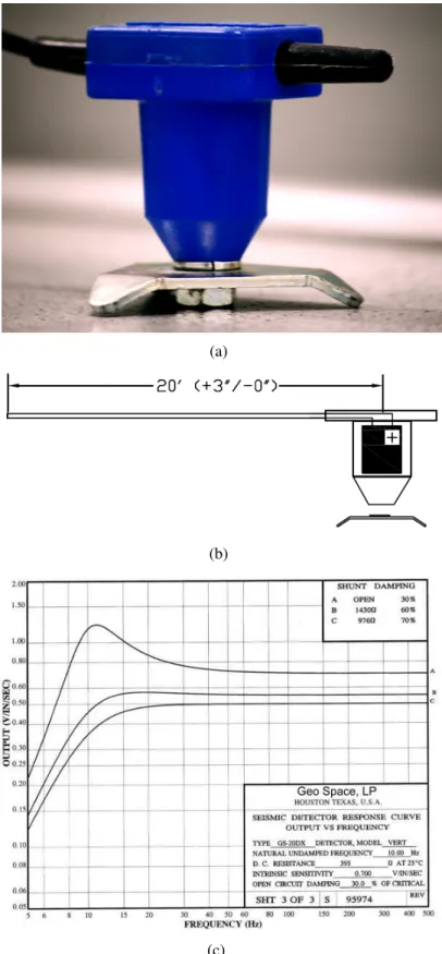
Six GS 20DX geophones were used for the experiments. The electrical details of a typical sen-sor [31] are depicted in Figure 2.1(b) and the frequency response curve is depicted in Figure 2.1(c). Transduction is achieved by means of a moving coil over a magnetic core. The

geo-phones are designed to be floor mounted. Floor to sensor contact was achieved by means of a coupling bolt screwed to the sensor, which was held to the floor by means of a tripod base. This was done since tight coupling was not feasible as it requires structural penetration by means of a probe.

The sensors constitute a wired suite and are connected to a data-acquisition system (DAQ). The DAQ is essentially an AD converter with preset amplification and low level software for de-vice control. The DAQ used for these experiments was a model PDL-MF: a PCI data-acqusition device developed by United Electronic Industries, Walpole, MA. The data-acquisition card pro-vides for 8 analog input channels with an overall sampling rate of 50,000 samples/s and 16-bit quantization. At its maximum preset amplification factor of 10 it can faithfully (i.e., without clipping) digitize a signal of amplitude _±1V. While lower amplifications can accommodate a wider range of signal amplitude, this setting was selected as footsteps generate a voltage swing, in each sensor, of the order of only a few mV.

The DAQ was programmed, using a C++ library provided by the manufacturer, to acquire data at 5kHz. The DAQ was programmed on a non-real-time operating system (Microsoft Windows XP Professional) and therefore, file I/O operations for a 5kHz sampling rate is a challenging task. Sequential read-write execution leads to the read buffer in the AD converter getting filled up before the acquired data can be written, leading to data loss. This problem exists in spite of the manufacturer providing a large capacity circular buffer. The problem was solved by programming the read and write operations to execute as parallel threads.

2.2

Experiments

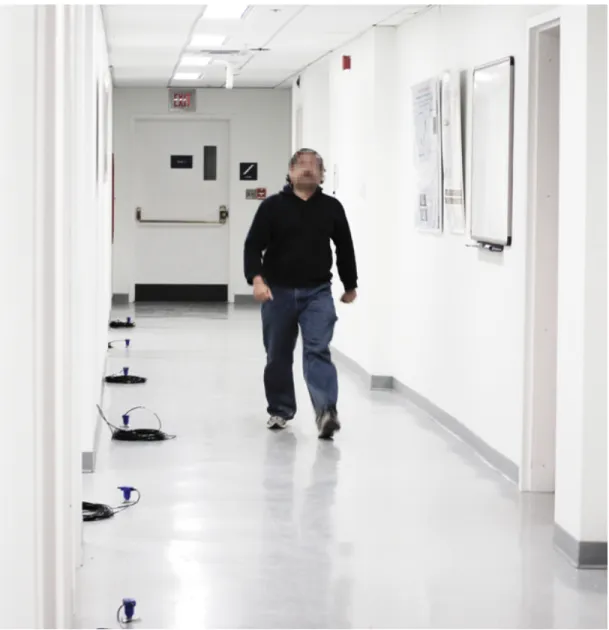
The six sensors were configured as a linear array. They were placed along the long edge of a hallway (see Figure 2.2). Data was collected in two (different) building hallways of similar construction. The sensors were placed along the long edge of the hallway. The distance be-tween adjacent sensors was maintained at 5ft. The rationale for selecting a sampling rate of

(a)

(b)

(c)

Fig. 2.1: The GS 20DX geophone. (a) Sensor as housed and packaged (b) Electrical details: cable length and sensor polarity (c) Frequency response curve.

5kHz was so that, if necessary, high frequency information in the footstep data [29] could be utilized for detection/classification. However, considering the frequency response curve of the GS 20DX (see Fig. 2.1(c)) and the typical quasi-periodicity of footstep signals, the raw signal was uniformly down-sampled to 1024 samples/second.

Background data was collected by leaving the sensors in an isolated environment. Back-ground data is approximately of a 4 minute duration. Multiple persons participated in the footstep data collection. The footstep data collected consists of 120 single-person trials (i.e., a given trial has exactly one participant walking along the hallway) and 120 two-person trials (a given trial has exactly two participants walking along the hallway). Each dataset consists of 60 trials from Building 1 and 60 trials from Building 2. The approximate duration of the data collected per trial is 12 seconds. The background and footstep signal from a single person trial are graphed in Fig. 2.3 and Fig. 2.4 respectively. In the following section, some analysis on data collected is presented, the analysis focuses on the presence of nonlinearity and heavy tailed behavior of the seismic data.

2.3

Preliminary data analysis

In this section, we present an analysis of the data. The nonlinear nature of the data is first ex-plained. Signal nonlinearity, within the footsteps context, is strongly suggestive of a nonlinear mixing medium of signal propagation. The tail behavior of the data is analyzed next, and we demonstrate that the footstep data cannot be explained by a Gaussian or exponential tail-decay model.

2.3.1

Nonlinearity analysis of observed data

A signal y(t)is said to be nonlinear if its current value cannot be predicted or expressed as a linear function of its past values. Let i denote the sensor index, i.e., i = 1,2, . . . ,6. Each

1000 2000 3000 4000 5000 6000 7000 8000 9000 10000 −2 0 2

x

x

x

x

x

x

1000 2000 3000 4000 5000 6000 7000 8000 9000 10000 −2 0

x

x

x

x

x

x

Fig. 2.4: Time series of a footstep trial. Nonstationarity and the impulsive nature of the signal is evident.

sensor observation, yi(t), is uniformly down-sampled to 1024 Hz. Each yi(t)is divided into 1 second overlapping frames. Denote by_Tr, the set of all time instants contained in the rth frame. Therefore, the cardinality of_Tr,|Tr|, is 1024. The inter-frame overlap was set to 50%.

The method of surrogate data [82] is used to analyze the acquired seismic time series for the presence of nonlinearity. The null hypothesis states that the original time series is a real-ization of a linear Gaussian process (or monotonic transforms thereof). The idea is to generate a set of time series (surrogate data set) by resampling from the original measurements so that linear statistical properties of the original data are preserved in the surrogate data set. These surrogates are then, in essence, samples from a population consistent with the null hypothesis of linearity and can be used to estimate the distribution of a test statistic that can discrimi-nate between the null (linearity) and alternative (nonlinearity). This statistic is computed for both the surrogate data and the original time series. If the statistic computed on the original time-series lies (significantly) in the tail of the distribution of the statistic corresponding to the surrogate, the null is rejected.

Following Schreiber [82], a third order statistic,

φrev ₌ 1 N ₋1 N X n=2 (y[n]₋y[n₋1])3_{, (2.1)}

is used to test for nonlinearity in our analysis. Herey[n]is the sampled version ofy(t)andN is the number of samples in ther-th frame. A known property of a linear Gaussian process is that its statistics are symmetric under time reversal [103]; φrev _{measures the asymmetry of a} series under time-reversal [82].

Each frame ofyi(t) (for all i) is tested for the presence of nonlinearity as follows. Forty surrogates, sk(t) : k = 1,2, . . . ,40, are generated from a given frame of the original time seriesyi(t)using the iterative amplitude adjusted Fourier transform (IAAFT) [82]. The IAAFT algorithm is based on the amplitude adjusted Fourier transform (AAFT) algorithm [93], which samples from a normal distribution and the sampled sequence is ranked and scaled so that the

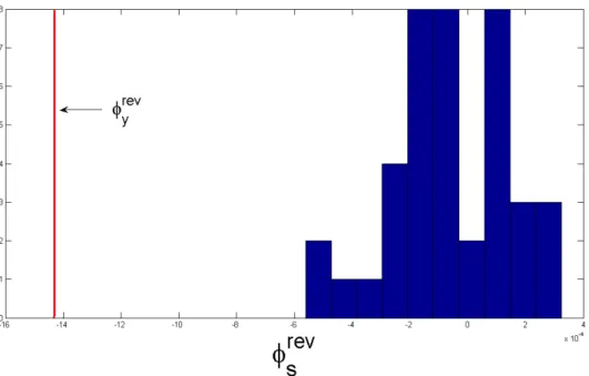
Fig. 2.5: Test for nonlinearity. Histogram is generated using the surrogate data. The statistic of the original time series is represented by the solid line labeledφrev

y .

amplitude spectra of the surrogates matches that of the frame under test while randomizing the phase uniformly between 0 and 2π. Schreiber notes that the AAFT algorithm is correct only

asymptotically: it generates surrogates that are linearandhave the same amplitude probability distribution (APD) as the original time-series asN → ∞. The IAAFT algorithm, proposed in [83], iterates between amplitude adjustment and phase randomization until the surrogates and the original data have the same APD. The statistic in Eq. (2.1) is then computed for both the surrogates and the test data. For example, consider Fig. 2.5. The solid line indicates the value ofφrev

y , the statistic computed for sensor data corresponding to a frame from the walking trials. The histogram ofφrev

s , computed for the corresponding surrogates is also shown. It is evident that the footstep signal has a nonlinear structure to it asφrev

y does not lie within the distribution of the null hypothesis corresponding to linearity. Thus, the null hypothesis can be rejected.

Each frame of the footstep signal is tested for the presence of nonlinearity at0.05 signifi-cance level(α= 0.05)using a rank order test proposed by Theiler et al. (see Section 2.1, [93]).

Table 2.1: Percentage of frames detected as nonlinear.

Sensor Footstep data

i 1 sframe 2 sframe 1 25 20 2 19 26 3 12 14 4 11 11 5 17 20 6 19 24

The case when the frames are two seconds in duration is also considered and results are summa-rized in Table 2.1. We observe that a significant proportion of the walking frames are detected as nonlinear. However, the exact nature of the nonlinearity is not known and is difficult to ascertain. This, is also a different characterization of the nonstationarity present in the data, and therefore, motivates the use of semiparametric methods of inference with such data. We also compared the values ofφrev _{obtained for the footstep and background data. The standard} tests for normality, such as the Jarque-Bera test, confirm that the background data are normally distributed. After standardizing the footstep and background time-series data, values ofφrev are computed over 1s and 2s frames. In Table 2.2, φ¯rev_{, the mean value of φ}rev _{over the total} number of frames, along with the standard error (SE_φ¯rev) are shown for both frame durations. Similar to what we observe in Fig. 2.5, the numbers reveal that for a linear Gaussian process, values of φ¯rev _{are close to zero with narrow standard errors, implying that the values of φ}rev are spread about a narrow interval centered about0. Values ofφrev_{for the footstep data, on the} other hand, lie significantly outside this region and are almost an order of magnitude greater than the typical φ¯rev _{values for linear Gaussian processes. However, since φ}¯rev _{estimates for} footstep data also possess larger standard errors, several time-series frames are classified as “linear” as seen in Table 2.1.

i 1 sframe 2 sframe 1 sframe 2 sframe 1 −0.0050 −0.0035 −0.0185 −0.0115 [12.67·10−5_{] [5.4·10}−5_{] [6.1·10}−4_{] [3.5·10}−4_] 2 0.0005 0.0004 0.1557 0.0938 [1.6_·10−5_{] [0.8·10}−5_{] [4.6·10}−3_{] [2.7·10}−3_] 3 ≈ −10 −5 _{≈ −10}−5 _{0.0120 0.0139} [2.2·10−5_{] [1.3·10}−5_{] [4.3·10}−4_{] [2.9·10}−4_] 4 −0.0010 −0.0013 0.0205 0.0248 [2.7_·10−5_{] [1.8·10}−5_{] [7.2·10}−4_{] [4.9·10}−4_] 5 −0.0003 −0.0003 0.0147 0.0176 [2.3·10−5_{] [1.3·10}−5_{] [6.3·10}−4_{] [4·10}−4_] 6 −0.0080 −0.0084 0.0056 0.0079 [7.6_·10−5_{] [6.1·10}−5_{] [5.2·10}−4_{] [3.1·10}−4_]

2.3.2

Tail behavior of the seismic data

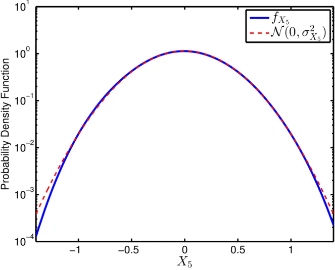
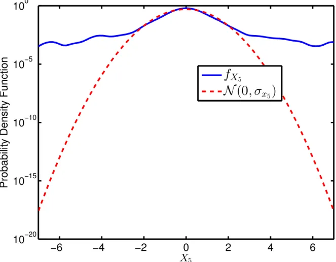
We have also analyzed the collected seismic data for the tail behavior. The background data show the presence of exponential tails, and the footstep data show the presence of heavy tails which decay at a polynomial rate. An example of this tail behavior is shown in Fig. 2.6 and Fig. 2.7. We observe that not only do the tails of the background data have exponential decay, but they do this at a slightly sub-Gaussian rate. This can be explained considering the physical nature of the geophone, which damps sudden (discontinuous) excursions of the signal. An idea of this behavior can also be inferred from the frequency plot of the sensor in Fig. 2.1, which shows a damped response in the high-frequency regime. On the other hand, the heavy-tailed behavior of the footstep data is clearly visible in Fig. 2.7. In fact, we can even infer a polynomial decay in the tails of the footstep data. Note that for any distribution decaying at a polynomial rate in the tails, i.e., as_|x_|−α−1_{, the logarithm of this, i.e.,−(α+ 1) log|x|will}

−1

−0.5

0

0.5

1

10

10

10

10

10

10

X

Probability Density Function

f

N

₍₀

_,

σ

X5

)

Fig. 2.6: Probability distribution of the background data from Sensor 5, compared to the p.d.f. of normal distribution with the same second-order moments as the background data. The Y-axis is plotted on a logarithmic scale.

for footstep data, where theY-axis is plotted on a logarithmic scale. The significance of a tail decay rate of_|x_|−α−1 _{is explained in Chapter 4.}

2.4

Other datasets

The research in this dissertation took place in collaboration with US Army Research Laboratory (ARL). In this effort, we also collected data using the unattended ground sensor (UGS) suite at ARL, at Adelphi, MD. Additional data, for an outdoor scenario, was collected by ARL near the

−6

−4

−2

0

2

4

6

10

10

10

10

10

X

Probability Density Function

f

N

₍₀

_,

σ

5

)

Fig. 2.7: Probability distribution of the footstep data from Sensor 5, compared to the p.d.f. of normal distribution with the same second-order moments as the footstep data. TheY-axis is plotted on a logarithmic scale.

southwest US border. The copula-based methods, proposed in Chapters 4 and 5, have also been applied to these datasets. For the purpose of demonstrating our detection methodology on real sensor data, in this dissertation, we focus on the results obtained using the dataset described in this chapter. However, we have applied similar methods to the indoor and outdoor ARL datasets and results based on these data are discussed in Chapter 6.

2.5

Summary

In this chapter we analyzed the nature of seismic data collected using geophone sensors in an indoor environment. The analysis revealed that the data corresponding to footstep activity exhibits temporal nonlinearity, with heavy-tailed behavior. The background data, on the other hand, are approximately normal. Time series plots of the footstep data also reveal that the data are spatially dependent, but signal nonlinearity will imply that the statistical dependence exhibited by the data will not be explainable by simple models. A more sophisticated under-standing of statistical dependence is required, and appropriate models must be used for any sort of inference done using such data. While we have demonstrated the existence of complex spatio-temporal behavior using footstep data, such signal characteristics can be seen in other types of data too. The analyses presented in this chapter, therefore, motivate our research ap-proach in this dissertation. We address the general theory of detecting such spatially dependent heavy-tailed data, and return to the footstep data example to apply our proposed methods.

C

HAPTER

3

S

TATISTICAL

D

EPENDENCE AND

C

OPULA

T

HEORY

Chapter 1 reviewed the recent research on signal processing for stochastically dependent obser-vations. As noted in Section 1.4, parametric, semi-parametric and non-parametric techniques of dependence characterization have been extensively studied, and they find utility in a variety of applications. As a consequence, research that includes the consideration of dependence in various disciplines such as machine learning, information theory, speech processing, finance, and aerospace, among others, has led to a rich body of literature. Dependence modeling, in this dissertation, is based on copula theory, which can be categorized as either a parametric or semi-parametric approach to dependence modeling, depending on the formulation being considered. In this chapter, concepts and measures of dependence are discussed (Section 3.1), followed by an overview of copula theory (Section 3.2).

3.1

Bivariate statistical dependence

The topic of stochastic dependence has been studied extensively since Karl Pearson first de-fined the product-moment correlation. This section discusses several concepts and measures of bivariate dependence that have since sought to generalize Pearson’s correlation coefficient. The focus on bivariate dependence is due to the fact that many concepts of multivariate dependence do not carry over as a simple extension of the bivariate case. Further, when exploring the idea of multivariate dependence, we use a pairwise scheme, in Chapter 5, based on the concept of

vines. The topics covered here summarize a more detailed treatment of dependence concepts by Balakrishnan and Lai (see [7], Chapter 3 and Chapter 4). The discussion that follows in the next section will show how a copula-based characterization of joint distributions relates to these generalized descriptions of dependence.

3.1.1

Positive and negative dependence

For two continuous random variables, X andY, positive dependenceimplies that large/small values ofY tend to accompany large/small values ofX. In contrast,negative dependence im-plies that large/small values ofY tend to accompany small/large values ofX. We discuss only concepts that are derived from positive dependence, since the negative dependence counter-parts are analogous. Further, if the pair(X, Y)has a positive dependence, then (X,−Y)has negative dependence onR2_{. If there exists a constraint of positivity,(X,1−Y)has negative}

dependence on the unit square. An important point to note is that while one may define posi-tive dependence for the multivariate case, negaposi-tive dependence is no more a mirror reflection of positive dependence. Six basic conditions describing positive dependence have been discussed in the literature [55]. These are enumerated below in the increasing order of stringency.

1. Positive correlation. Defined for positive linear correlation, i.e.,cov(X, Y)≥0.

aandbdefined onR2 _{which are increasing in each of the arguments separately,}

cov[a(X, Y), b(X, Y)]≥0.

Lai and Xie note that a direct verification of association is difficult [55]. It is often simpler to verify one or more of the conditions to follow, which are more stringent, and thus, imply association.

4. Tail dependence. Y is right-tail increasing in X, denoted as RTI(Y|X), if P(Y > y|X > x) increases in xfor all y. Similarly,Y is left-tail decreasing in X, written as

LTD(Y_|X)ifP(Y _≤y_|X _≤x)decreases inxfor ally.

5. Stochastically increasing (SI). Y is said to be stochastically increasing in x for ally,

SI(Y_|X), if for everyy,P(Y > y_|X =x)is increasing inx. SI(X_|Y)can be defined in a similar manner. IfY is SI inX,E(Y_|X =x)is also increasing inx.

6. Total positivity of order 2. LetXandY have a joint densityf(x, y). Thenf is said to be totally positive of order 2 (TP2) if for allx1 < x2, y1 < y2,

f(x1, y1)f(x2, y2)≥f(x1, y2)f(x2, y1)

TP2is also referred to asXandY being likelihood ratio dependent (LRD).

Since these conditions were listed in the increasing order of stringency, (6) _⇒(5) _⇒ (4) _⇒ (3)_⇒(2) _⇒(1). When the inequality signs of the relations described in (1) through (6) are reversed, we obtain analogous negative dependence concepts. Specifically, the duals of (2), (4), (5) and (6) are respectively called negative quadrant dependent, right tail decreasing/left

tail increasing dependence, stochastically decreasing dependence and reverse regular of order 2.

3.1.2

Measures of dependence

Measures of dependence quantify, in some particular manner, how closely the variablesX and Y are related. Since a single number alone cannot completely explain the nature of depen-dence, a variety of measures are defined and used. The following list is not comprehensive, but represents some of the more important measures of dependence that have been proposed.

1. Pearson’s correlation. This is a well studied measure in statistics and is presented here for completeness. Pearson’s coefficient of correlation is given by,

ρ= pcov(X, Y)

var(x) var(Y)

It may be noted that ρ measures only the linear dependence. Furthermore, there exist well-known examples whereX andY are dependent, butρ= 0. For example, Melnick and Tenenbein [62] have analyzed the following case. Let X _{∼ N}(0,1)and defineY such that forλ >0

Y =        X if _|X_{| ≤}λ −X if _|X_|> λ (3.1)

We can verify thatY _{∼ N}(0,1), since

P(Y ≤t) = P(|X| ≤λ∧X ≤t) +P(|X|> λ∧ −X ≤t) (3.2)

=P(|X| ≤λ∧X ≤t) +P(|X|> λ∧X ≤t)

=P(X _≤t). (3.3)

ρ =E[XY] = 2 0 x fX(x)dx−2 λ x fX(x)dx = 4 Z λ 0 x2_f X(x)dx−1 (3.4)

Solving forλby settingρ= 0in (3.4), Melnick and Tenenbein have obtainedλ_≈1.54; for this value ofλ, in spite ofX andY being dependent,ρ = 0. Note thatX andY are notjointlynormal, i.e.,fXY is not a bivariate normal p.d.f., and hence their dependence structure is not completely explained byρ.

2. Mutual information. Mutual information betweenX, Y is defined as,

I(X;Y) = Z R2 log fXY(x, y) fX(x)fY(y) dFXY(x, y),

and it measures the distance between the joint density and the product of marginals, i.e., the joint density if X, Y were independent. Multiinformation is the multivariate extension of mutual information proposed by Joe [40]. For the vectorX_∈Rn_{, n >2,}

I(X) = Z Rn log fX(x) Q ifXi(xi) dFX(x).

A normalization of the formδ∗ ₌p

1₋exp(₋2_I)ensures that mutual information and multiinformation follow Rényi’s postulates [77] for “an appropriate measure of depen-dence”. In particular,δ∗ _∈[0,1].

3. Rank correlations.Rank correlations measure the dependence between rankings, rather than between actual values, ofXandY. Therefore, rank measures are unaffected by any increasing transformation of X andY, whileρis unaffected only by linear transforma-tions. Kendall’s tau (τ) and Spearman’s rho (ρS) are widely used measures that fall in this category. For independent pairs of random variables (X1, Y1)and (X2, Y2)having the

same distribution as(X, Y), concordance is defined as the condition that(X1−X2)(Y1−

Y2) _≥ 0 and discordance is defined as the condition that (X1 −X2)(Y1 − Y2) < 0.

Kendall’s tau is defined to be the difference between the probabilities of concordance and discordance:

τ ,P[(X1−X2)(Y1−Y2)≥0]−P[(X1−X2)(Y1−Y2)<0].

This definition is equivalent to,

τ = cov[sgn(X1−X2),sgn(Y1−Y2)].

Kendall’s tau is also a measure of total positivity: τ /2represents an average measure of the total positivity forfXY, the joint density ofXandY.

Spearman’s rho is defined as follows. Let(Xi, Yi), i= 1,2,3be three independent pairs of random variables with a common distribution function. Then,

ρS ,3{P[(X1−X2)(Y1 −Y3)≥0]−P[(X1−X2)(Y1−Y3)<0]}.

Spearman’s rho represents an average measure of quadrant dependence: ρS ≥ 0 ⇒ (X, Y)are PQD.

4. Blomqvist’s β. This measure evaluates the dependence at the center of a distribution, where the center is defined by(˜x,y˜), the medians of the two marginals. Hence,βis also referred to as the medial correlation coefficient. Blomqvist’sβis defined as,

β = 2P[(X₋x˜)(Y ₋y˜)>0]₋1 (3.5)

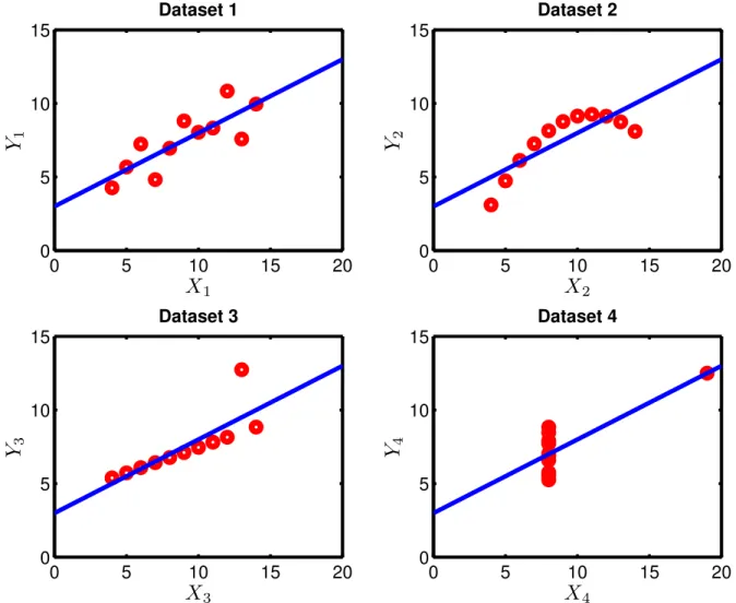
structed to demonstrate the importance of graphing data before analyzing it, the dataset also reveals the global nature of ρ, i.e., it is defined from the second moment, which is in turn an expectation evaluated over the entire plane. In other words, while global summary statistics are useful descriptors of the data, they often fall short of providing a complete picture about the true variability that exists in the data set. In fact, all of the above measures are global measures. Pairs (X, Y) and(X0_{, Y}0₎

can have different distributions and yet have the same global measure. A local measure of dependence will allow one to compare the variation of dependence between the two pairs. Several local measures of dependence have been proposed in the literature, mostly as an extension of global dependence measures. Some of them are listed below.

• Local correlation coefficient. Let µ(x) = E(Y|X = x), σ2_{(x) = var(Y|X = x)}

andβ(x) = ∂

∂xµ(x). The local correlation coefficient is then defined as

ρ(x) = σXβ(x) [σXβ(x)]2+σ2(x)

,

whereσX is the standard deviation ofX. When defined in this manner,ρ(x)shares a few properties with its global counterpart: it takes values between 1 and -1, in-dependence of X and Y implies that ρ(x) = 0 and ρ(x) = _±1 for almost all x is equivalent to Y being a function ofX. It is also invariant to scaling, but is not marginal free. The latter point means that if we defineU =FX(x)andV =FY(y), the resultingρ(u)is different fromρ(x).

• Localτ andρS. Local measures of rank correlation exist, and are evaluated on an open neighborhood about a point of interest,(x0, y0). The functional form is more

0 5 10 15 20 0 5 10 15

X

Y

X

Y

X

Y

X

Y

Fig. 3.1: Anscombe’s quartet. All 4 datasets contain identical summary statistics: Mean of Xi, µXi = 9, variance of Xi, σ 2 Xi = 11; mean of Yi, µYi = 7.5, variance of Yi, σ 2 Yi = 4.12; correlationρ= 0.816_∀i= 1,2,3,4.