Load forecasting using combination model of multiple linear regression with neural network for Malaysian city

http://dx.doi.org/10.17576/jsm-2018-4702-25

Load Forecasting using Combination Model of Multiple Linear Regression with

Neural Network for Malaysian City

(Peramalan Beban Menggunakan Model Gabungan bagi Regresi Linear Berganda dengan Rangkaian Neuron untuk Bandaraya di Malaysia)

Nur AriNA BAzilAh KAmisAN, muhAmmAd hisyAm lee*, suhArtoNo suhArtoNo, ABdul GhApor hussiN & yoNG zuliNA

zuBAiri

ABstrAct

Forecasting a multiple seasonal data is differ from a usual seasonal data since it contains more than one cycle in a data. Multiple linear regression (MLR) models have been used widely in load forecasting because of its usefulness in the

forecast a linear relationship with other factors but MLR has a disadvantage of having difficulties in modelling a nonlinear

relationship between the variables and influencing factors. Neural network (NN) model, on the other hand, is a good

model for modelling a nonlinear data. Therefore, in this study, a combination of MLR and NN models has proposed this

combination to overcome the problem. This hybrid model is then compared with MLR and NN models to see the performance

of the hybrid model. RMSE is used as a performance indicator and a proposed graphical error plot is introduce to see the

error graphically. From the result obtained this model gives a better forecast compare to the other two models. Keywords: Error plot; hybrid model; neural network; regression model; residuals

ABstrAK

Peramalan berganda data bermusim adalah berbeza daripada peramalan data bermusim biasa kerana ia mengandungi lebih daripada satu kitaran dalam satu data. Model berganda regresi linear (MLR) telah digunakan secara meluas dalam

ramalan beban kerana kegunaannya dalam meramalkan hubungan linear dengan faktor lain tetapi MLR mempunyai

kelemahan iaitu mempunyai kesukaran dalam memodelkan hubungan linear antara pemboleh ubah dan faktor yang mempengaruhi. Model rangkaian neural (NN) di sisi lain, adalah model yang baik dalam pemodelan data linear. Oleh

itu, dalam kajian ini gabungan MLR dan NN model dicadangkan gabungan ini untuk mengatasi masalah tersebut. Model

hibrid ini kemudiannya dibandingkan dengan MLR dan NN model untuk melihat prestasi model hibrid. RMSE digunakan

sebagai penunjuk prestasi dan plot ralat grafik diperkenalkan untuk melihat ralat secara grafik. Daripada keputusan yang diperoleh model ini memberikan ramalan yang lebih baik berbanding dengan dua model yang lain.

Kata kunci: Model hibrid; model regresi; plot ralat; rangkaian neural; sisa

iNtroductioN

TModelling a load forecasting is a very important task for electricity to function in a more efficient and safety way, give the most optimum cost for cost saving applications relying on operating reconstruction (Hahn et al. 2009; Soares & Medeiros 2008). By predicting the future load demands, power system planners and demand controllers could ensure that they would be enough supply of electricity to cope with increasing demands (Mastorocostas et al. 2000). For these reasons, load forecasting has attracted not only researchers but also organisation with same interest to forecast energy usage by using various methods from classical methods to the advanced methods.

Forecasting seasonal load demand has become increasingly challenging in recent period. Classical methods such as regression, holt winter’s and exponential smoothing are suitable for a large number of series, for

analyst with limited skill and also for a norm of comparison It follows certain pattern which was determined by the parameter of the model. But it is common for load data to contain a seasonal pattern. Because of these reasons, new models such as artificial neural network and fuzzy time series have been developed in order to find a better and accurate forecast for load forecasting (Chatfield 2005).

Modeling multiple seasonal loads is no longer optimal with standard seasonal methods. Multiple seasonal cycles is differ from the usual seasonal time series. In multiple seasonal cycles, it can contain two or more cycles. Malaysian data contain both daily and weekly cycles. Malaysia has many public holidays because of the ethnicity variation. The cycles from Monday to Friday are similar and Saturday and Sunday are quite discrete. And the patterns for public holidays are quite similar to weekends compare to weekdays. And as stated by Gould et al. (2008), the levels of the daily cycles may change from one week

to the next and yet it still highly correlated with the prior levels of the next day.

A simple or singular method can lead to a bias or inaccurate forecast (Basheer et al. 2014). Thus, a few research teams such as Basheer Shukur et al. (2014) and Mohamed and Ahmad (2010) have developed a hybrid model to deal with this double cycle problem. Some have also used a double seasonal ARIMA to overcome double

seasonal difficulties (Mohamed et al. 2011, 2010). Dudek (2016) proposed a linear regression model with patterns of daily cycle. The daily cycle is used as both input and output variables to eliminate the trend and seasonal cycles. Based on the results, the proposed method gives better outcomes compared to the ARIMA, exponential smoothing,

neural network and Nadaraya-Watson estimator models. Ringwood et al. (2001), Taylor (2003), Xiaojuan et al. (2010) and Zhang et al. (2008), even though they advocate the usage of the single model whether the advanced or traditional one, they have also suggested in their further works to consider a hybrid technique because it could improve the outcomes. This method is also being promoted by other researchers like Ying and Pan (2008) and Jang (1993). In this study, a hybrid model combination of multiple linear regression model and neural network will be considered.

The idea of developing this hybrid model comes from Zhang (2003). As mentioned by him, a real data never really consist from pure linear or nonlinear but always contain both linear and nonlinear. Often residuals are being neglected from being considered in analysis. Residuals are important in order to check whether a model is able to fit with a data. Although there is no general statistical diagnostic on how to detect nonlinear autocorrelation relationship but residuals can be concluded in a diagnosis to ensure that both linear and nonlinear part is consider (Zhang 2003). But all in all, the aim is to find a method that can yield a low error for the combined forecasts (Bates & Granger 1969) and the choices of appropriate method is depend on the context, the objectives, the analyst’s skill, data characteristics and the number of series to be forecast (Chatfield 2000).

The Holt-Winters method is widely used in practice. It has the advantage of being simple (Chakhchoukh et al. 2011) as it easily copes with trends and seasonal variation (Chatfield 1978). Holt Winter’s or multiple linear regression are suitable for a large number of series, given an analyst with limited skill and also for a norm of comparison (Chatfield 2000). It is appropriate to use when parameters stay persistent over time (Bowerman et al. 2005). It is also useful to explore the factors that influence the unusual fluctuations of the data (Ismail et al. 2008). Regression models are widely used for electricity load forecasting. Load is represented by a linear combination of variables related to the weather factors, day type, and customer class (Kyriakides & Polycarpou 2007). It is also appropriate to forecast time series with trend and seasonal factors as they may change over time (Bowerman et al. 2005). Multiple linear regression (MLR)

assumes that a regression model employ more than one

independent variable. In regression model, load data will be represented as a linear combination of variables related to other factors and in this study it is the day type (Kyriakides & Polycarpou 2007). But regression model often suffer from a number of difficulty due to a nonlinear relationship between load demand and the influencing factors (Kyriakides & Polycarpou 2007).

Since neural network is a flexible model in modeling a nonlinear data, it will be used to analyse the residuals that will be obtained from the MLR model. Neural network

has the competence and accessibility in estimated nonlinear data. It captures some of the key properties which replicate the models of biological neurons works (Bates & Granger 1969; Jang 1993; Kyriakides & Polycarpou 2007; Ringwood et al. 2001; Taylor, 2003; Xiaojuan et al. 2010; Ying & Pan 2008; Zhang 2003; Zhang et al. 2008). Due to this issue, a combination with neural network (NN) is

considered in order to enhance the forecast.

methods

The idea of the hybrid model came from Zhang (2003). In this study, a hybrid model combination of two models together. The first model will be used to forecast the output data and the second model will be used to forecast the residuals output from the first model. MLR model is

selected because of the suitability in modelling a consistent parameter over time. In this case, the parameters will be the days since the data have been arranged into 24 sets of independent series of data. Neural network will be combined with MLR model because of its benefit in

modelling a nonlinear data. As being stated by Zhang (2003), the relationship between an actual value and a forecasting can be written as:

yt = ŷt = εt, (1)

where yt is the actual value, ŷt is the forecasted value and

εtis the error or residual. From this equation, the ŷt will

be calculated by using MLR model and the error term or

residual, εt will be forecast by using NN model.

MLR model employ more than one independent

variable. The linear regression model relating y to x1, x2,

K, xk is:

y = μy|x1,x2,K,xk + ε = β0 + β1x1 + L + βkxk + ε, (2)

where μy|x1,x2,K,xk = β0 + β1x1 + L + βkxk is the mean

value of the dependent variable y when the values of the independent variables are x1, x2, K, xk. β0 + β1 + L + βk

are (unknown) regression parameters relating the mean value of y to x1, x2, K, xk. ε is the error term that describes

the effects on y of all factors other than the values of the independent variables x1, x2, K, xk.

In this study the linear regression model can be written as:

y = μy|x1,x2,K,xk + ε = β0 + β1x1 + L + β7x7 + ε, (3)

where x1, x2, K, x7 are dummy variables where x1 is

Monday, x2 is Tuesday and so on since the data used in this

MLR, the residuals obtained from the in-sample forecast

of MLR will be analyse by using neural network in Matlab

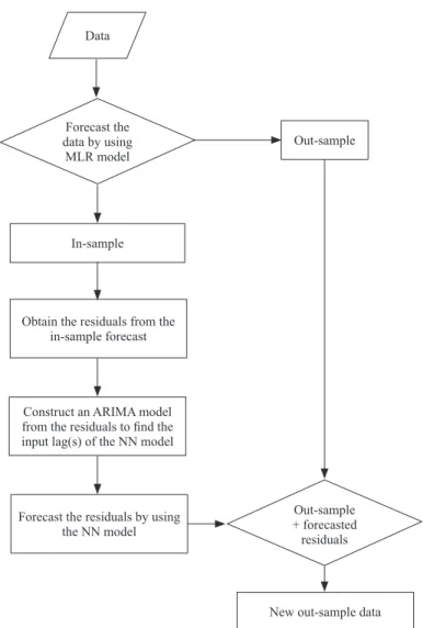
software. A two-layer feed-forward network with sigmoid hidden neurons and linear output neurons will be used in the neural network process. The network will be trained with Levenberg-Marquardt backpropagation algorithm and if there is not enough memory, scaled conjugate gradient backpropagation will be used to train the network. The step by step process of the process can be written as follows: First step: Data is modelled by using the MLR model.

Second step: Residual obtained from the in-sample forecast is calculated and the ACF and PACF of the

residuals are plotted to find the lags. If the lags are not stationary, then the residuals will be difference to 1 to make the ACF and PACF lags stationary. The lags obtained

will be used as the input nodes that will be used in the next process. Third step: Neural network model is then used to model the out-sample forecast of the residual. Forth step: The final out-sample forecast is obtained by adding the out-sample forecast from the MLR model with

the out-sample forecast of the residuals obtained from the neural network modelling process.

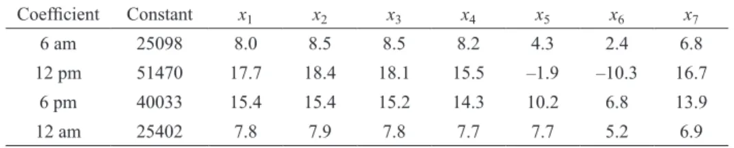
The results of the point estimated for the parameters are listed in the Table 1 below. The parameters x1 represent

Monday, x2 represents Tuesday and so on until x7 represent

Sunday. The parameters estimation of the MLR model can

be written as:

For example, we could write the equation of the MLR

model of 6 am as:

y = 25098 + 8.0x1 + 8.5x2 + 8.5x3 + 8.2x4 + 4.3x5

+ 2.4x6 + 6.8x7 (4)

The input lags in neural networks are determined based on autoregressive (AR) term in Box-Jenkins model.

Park et al. (1996), Tang and Fishwick (1993) and Zhang and Qi (2005) suggested that lags can be determined by the

AR terms and ignoring the MA terms. Based on the ACF and PACF plots of the residuals, the best Box-Jenkins model is

either ARIMA(0,1,1) or ARIMA(2,1,1) or ARIMA(2,1,2). The

model for ARIMA(0,1,1) can be written as:

(1 – B)yt = (1 – θ̂B)at

yt – yt–1 = at – θ̂at–1 (5)

yt = yt–1 + at – θ̂at–1,

and for ARIMA(2,1,1) can be written as:

(1 – B)yt = (1 – θ̂B – θ̂B2)at

yt – yt–1 = at – θ̂at–1 – θ̂at–2 (5)

yt = yt–1 + at – θ̂at–1 – θ̂at–2,

and for ARIMA(2,1,2) can be written as:

(1 – B – B2_)y

t = (1 – θ̂B – θ̂B2)at

yt – yt–1 – yt–2 = at – θ̂at–1 – θ̂at–2 (5)

yt = yt–1 + yt–2 + at – θ̂at–1 – θ̂at–2.

Since only the AR terms need to be considered to

choose the input lags, by ignoring the term in (4), the input lags to be considered are lag 1 and for (5) and (6), the input lags are 1 and 2. The input lags will be used to forecast the out-sample of the residuals of the NN model.

The number of neuron could influence the performance of MLP forecast performance. However, using minimum

number of neuron is most recommended (Masters 1993). Each neuron is processing unit that used logistic function to calculate the linear combination of inputs. The number of the nodes in the hidden layer could be decrease or increase based on the performance of the network training. In this study, the number of neurons that used is one up to five neurons. But in this study only the one that show the best performance will be discussed and only out-sample forecast is consider since the proposed method only appropriate for the out-sample forecast. For the proposed model, the step by step diagram on how the model working is shown in Figure 1 below.

This method is done by using Minitab and Matlab program. The MLR modeling part is done by using the

Minitab software while the NN modeling part is done by

using Matlab software.

TABLE 1. Parameters estimation for multiple linear regression model

Coefficient Constant x1 x2 x3 x4 x5 x6 x7

6 am 25098 8.0 8.5 8.5 8.2 4.3 2.4 6.8

12 pm 51470 17.7 18.4 18.1 15.5 –1.9 –10.3 16.7

6 pm 40033 15.4 15.4 15.2 14.3 10.2 6.8 13.9

12 am 25402 7.8 7.9 7.8 7.7 7.7 5.2 6.9

TABLE 2. Input lags for number of nodes in NN

Hour ARIMA model Lags

6 am (2,1,2) 1,2

12 pm (0,1,1) 1

6 pm (2,1,1) 1

GooDneSS-oF-FIT TeSTS

Root mean square error (RMSE) is used as the performance

indicator in order to see the performance of the model other than the comparison plot to observe the goodness-of-fit of the hybrid model. The smaller the number of the RMSE

indicates the better the model is. RMSE is preferred compare

to MSE because of their theoretical relevance in statistical

modelling. often, the RMSE is preferred to the MSE as it is

on the same scale as the data (Hyndman & Koehler 2006). The formula of the RMSE can be seen as:

RMSE =

√

Σ

t=1

(

y

– ŷ

)

2_{, (8)}

where ŷt is the predicted value and yt is the observed value.

Other than RMSE, we also suggested an error plot in

order to compare the results and to determine whether a hybrid model should be considered or not. Usually, plot of error or residual plot is used to see the error graphically. But the problem with residual plot is that it depends on the value from the data. If the data has large number, then the number error could also give a big value which will affect the point in the residual plot. The proposed plot will transform the value of data into percentage by using the formula in order to standardize the value.

xt =

|

t

|

xt is the percentage value that will be used in the plot and

the value will be between 0 and 1, yt is the actual value

and ŷt is the forecast value. Since the data is in thousand

kilowatt, the error given by RMSE will give a large value.

To support the number from RMSE, the MAPE is also used

because MAPE will give value in percentage which is more

understood where the highest value will be 1 and smallest will be 0. The MAPE is given by this formula:

1– n n

Σ

|

|

where yt is the actual value and ŷt is the predicted value.

For all of the above three performance indicators, the smaller the value and the closer it is to zero, the better is the predicted model in fitting the observed data. note that the values cannot be negative, since all of the formulas use the modulus or square of the values.

THe DATA SeT

We used a data from Tenaga Nasional Berhad Johor Bahru. Data were recorded every day for 3 years from a station

FIGURE 1. Process of how the proposed method performs the forecast Out-sample

Data

Forecast the residuals by using the NN model Construct an ARIMA model from the residuals to find the input lag(s) of the NN model Obtain the residuals from the

in-sample forecast In-sample Forecast the data by using MLR model Out-sample + forecasted residuals

named Pusat Bandar Johor Bahru. Pusat Bandar Johor Bahru (PBJB) is a commercial area in Johor Bahru. Four

selected hours used in this paper are 6 am, 12 pm, 6 pm and 12 am. These four selected hours represent the peak hours and the dip hour in Johor Bahru and generally it can represent the daily scenario in Malaysia too.

For casual hours like 6 am and 12 am, there are not much differences of load usage between weekdays and weekends but for peak hours such as 12 pm and 6 pm the load usage during weekdays is higher compare to the weekend’s usage. These four hours are selected not only because of the high and low usage, but also to see the pattern and differences of the load usage between these hours.

resultANd discussioN

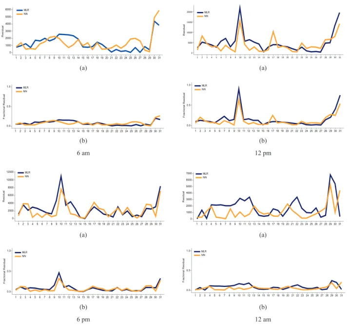
A comparison between residual plot and percentage error plot is discussed here. As can be seen from Figure 2,

residual plot do not have a fix scale on the y-axis. The scale on the y-axis depends on the value of the residual. Therefore, there is not much information gained from this plot. Compare to percentage error plot, the scale on the y-axis is fixed from 0 to 1. It is easier to determine whether the forecast is good or not. And one can set its own benchmark when making a decision to determine a good or bad forecast.

Other than using the percentage error plot as a comparison between models, it also could be used as a benchmark plot for certain purpose. In this study, we used this plot to determine whether a data need to be forecasted with hybrid or not. We set the benchmark at 0.4. If there is any point exceeds 0.4, a hybrid model will be considered. As can be seen from the figures below, 12 pm and 6 pm contain points which is greater than 0.4. To ensure that this rule could be applied, we test all of the data used in this study with the proposed hybrid model and compare it with the result in RMSE.

31 30 29 28 27 26 25 24 23 22 21 20 19 18 17 16 15 14 13 12 11 10 9 8 7 6 5 4 3 2 1 6000 5000 4000 3000 2000 1000 0 R es id ua l MLR NN 31 30 29 28 27 26 25 24 23 22 21 20 19 18 17 16 15 14 13 12 11 10 9 8 7 6 5 4 3 2 1 1.0 0.5 0.0 F ra ct io na l R es id ua l MLR NN 31 30 29 28 27 26 25 24 23 22 21 20 19 18 17 16 15 14 13 12 11 10 9 8 7 6 5 4 3 2 1 12000 10000 8000 6000 4000 2000 0 R es id ua l MLR NN 31 30 29 28 27 26 25 24 23 22 21 20 19 18 17 16 15 14 13 12 11 10 9 8 7 6 5 4 3 2 1 1.0 0.5 0.0 F ra ct io na l R es id ua l MLR NN 31 30 29 28 27 26 25 24 23 22 21 20 19 18 17 16 15 14 13 12 11 10 9 8 7 6 5 4 3 2 1 20000 15000 10000 5000 0 R es id ua l MLR NN 31 30 29 28 27 26 25 24 23 22 21 20 19 18 17 16 15 14 13 12 11 10 9 8 7 6 5 4 3 2 1 1.0 0.5 0.0 F ra ct io na l R es id ua l MLR NN 31 30 29 28 27 26 25 24 23 22 21 20 19 18 17 16 15 14 13 12 11 10 9 8 7 6 5 4 3 2 1 7000 6000 5000 4000 3000 2000 1000 0 R es id ua l MLR NN 31 30 29 28 27 26 25 24 23 22 21 20 19 18 17 16 15 14 13 12 11 10 9 8 7 6 5 4 3 2 1 1.0 0.5 0.0 F ra ct io na l R es id ua l MLR NN

FIGURE 2. A comparisons between residual plot (a) and fractional residual plot (b) for selected times

(a) (a) (b) 6 am (b) 12 pm (a) (a) (b) 6 pm (b) 12 am

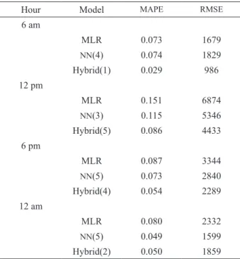
Here is the result of the hybrid model. 6 am, 12 pm, 6 pm and 12 am from Pusat Bandar Johor Bahru was selected for this purpose. Comparing the plots of percentage error above and the error measurement in Table 3 below, it is agreed that for 12 pm and 6 pm where there are points that exceed 0.4, hybrid model gives smaller value of RMSE and

for 12 am where all the points are below 0.4 in the plot,

NN shows smaller value of RMSE compare to hybrid model

which suggest that hybrid model is not necessary. As for 6 am, although all the points in the plot are below 0.4, hybrid model shows a smaller value of RMSE.

This is understood since 6 am represent the transition time when most people in Malaysia start their day. At this hour, they usually busy preparing their self to working and other activities. Therefore, transition hour should be considered to be tested with hybrid model. The result of the out-sample forecast can be seen in the figures and tables below. other than that, absolute error plot also shows that all forecast by using NN gives small error which could also suggest that it

is a good model if hybrid model is not used for this data. The result of the out-sample for selected hours can be seen in Table 3. Both tests show consistent results for the models of selected hours. For 6 am, 12 pm and 6 pm, the hybrid model gives a better result compare to other models. The RMSE for 6 am was reduce to almost 41.3% while when

data is forecasted with the hybrid model compare to MLR

and 46.1% was reduce for RMSE compare to NN model.

The RMSE for 12 pm reduce to almost 35.5% compare

to MLR and reduce 17.1% compared to NN model. As for

6 pm, the hybrid model also fit the data well compare to MLR and NN. A reduction in RMSE result can be seen

from Table 3.Other than using the absolute error plot as a comparison between models, it also could be used as a benchmark plot for certain purpose. In this study, we used this plot to determine whether a data need to be forecasted with hybrid or not. We set the benchmark at 0.4. If there is

any point exceeds 0.4, a hybrid model will be considered. As can be seen from the figures below, 12 pm and 6 pm contain points which is greater than 0.4. To make sure that this rule could be applied, we test all of the data used in this study with the proposed hybrid model and compare it with the result in RMSE.

Here is the result of the hybrid model. 6 am, 12 pm 6 pm and 12 am from Pusat Bandar Johor Bahru was selected for this purpose. Comparing the plots of percentage error above and the error measurement in Table 2 below, it is agreed that for 12 pm and 6 pm where there are points that exceed 0.4, hybrid model gives smaller value of RMSE and

for 12 am where all the points are below 0.4 in the plot,

NN shows smaller value of RMSE compare to hybrid model

which suggest that hybrid model is not necessary. As for 6 am, although all the points in the plot are below 0.4, hybrid model shows a smaller value of RMSE.

This is understood since 6 am represent the transition time when most people in Malaysia start their day. At this hour, they usually busy preparing their self to working and other activities. Therefore, transition hour should be considered to be tested with hybrid model. The result of the out-sample forecast can be seen in the figures and tables below. other than that, absolute error plot also shows that all forecast by using NN gives small error which could also suggest that it

is a good model if hybrid model is not used for this data. The MAPE shows a consistent result as the RMSE. For

hour 6 am, 12 pm and 6 pm, the hybrid model shows the smallest value of RMSE and MAPE which indicate that the

model is the best compare to MLR and NN models. Hour

12 am shows that NN with neuron 5 is slightly better

compare to hybrid model but from MAPE we could see

that the difference is only 0.001. Thus, from the error measurements results we could see that the hybrid model did improve the forecast of the load data. The more obvious pattern can be seen in figures below.

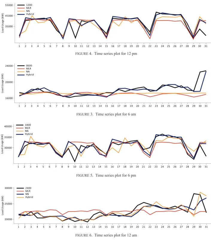
As can be seen from Figure 3, the outline of hybrid plot is closer to the actual plot outline compare to the other two plots. Although at certain point, the hybrid model could not detect the actual point, but as can be seen at point 31 in x-axis where there is a sudden increment in the load usage reading, the hybrid did follow the actual value pattern compare to the MLR or NN models. While for 12 pm, the

pattern of the load is more obvious where a sudden drop-off could be seen from the plot in Figure 4. This is understand as explained above, 12 pm is the peak hour and the sudden drop-off is actually the weekend when people are mostly not working and since this data cover the urban region, the pattern is obvious at 12 pm compare to the other three hours. From the figures above, it is obvious that the hybrid model gives better performance in following the pattern of the actual load compare to MLR and NN.

overall, as can be seen from Figures 3-5, NN and

hybrid give a quite identical plot and could read the pattern of the actual data. Although at certain time such as 12 am the hybrid model does not gives a good result, it can still be concluded that this hybrid model could be used to forecast the load data especially load data from Malaysia. NN is a

good model when forecasting a nonlinear data. As can

TABLE 3. error measurement of selected hours

Hour Model MAPE RMSE

6 am MLR 0.073 1679 NN(4) 0.074 1829 Hybrid(1) 0.029 986 12 pm MLR 0.151 6874 NN(3) 0.115 5346 Hybrid(5) 0.086 4433 6 pm MLR 0.087 3344 NN(5) 0.073 2840 Hybrid(4) 0.054 2289 12 am MLR 0.080 2332 NN(5) 0.049 1599 Hybrid(2) 0.050 1859

be seen from Figure 6, the load at 12 am did not show an obvious seasonal pattern compare to the others. Because of that, NN shows a superior result compare to hybrid model

for 12 am. However NN is also a good model in forecasting

the load compare to the traditional model, MLR. Therefore,

if ones do not wish to forecast by using the hybrid model,

NN model could be consider as an alternative model. coNclusioN

The hybrid model has shown to be superior compare to MLR

and NN models. The combination of MLR and NN is a good

combination especially for a data that has a similar pattern like Malaysian data. Malaysian data has a multiple seasonal

pattern since the data contain few cycles in the load and since regression can model a data with variable from other factor and NN is a good model in modelling a nonlinear

data, the combination of these two models could enhance the forecasting of the load. The percentage error plot is also a good plot to check the error graphically. It could give brief idea on whether a forecast is good or bad and it also can be used to make a comparison between models.

REFERENCES

Basheer Shukur, o., Salem Fadhil, n., Hisyam Lee, M. & Hura Ahmad, M. 2014. electricity load forecasting using hybrid of multiplicative double seasonal exponential smoothing model

31 30 29 28 27 26 25 24 23 22 21 20 19 18 17 16 15 14 13 12 11 10 9 8 7 6 5 4 3 2 1 30000 25000 20000 Lo ad U sa ge (k W ) 2400 MLR NN Hybrid 31 30 29 28 27 26 25 24 23 22 21 20 19 18 17 16 15 14 13 12 11 10 9 8 7 6 5 4 3 2 1 40000 35000 30000 Lo ad U sa ge (k W ) 1800 MLR NN Hybrid 31 30 29 28 27 26 25 24 23 22 21 20 19 18 17 16 15 14 13 12 11 10 9 8 7 6 5 4 3 2 1 24000 20000 16000 Lo ad U sa ge (k W ) 0600 MLR NN Hybrid 31 30 29 28 27 26 25 24 23 22 21 20 19 18 17 16 15 14 13 12 11 10 9 8 7 6 5 4 3 2 1 55000 45000 35000 Lo ad U sa ge (k W ) 1200 MLR NN Hybrid

FIGURE 3. Time series plot for 6 am

FIGURE4. Time series plot for 12 pm

FIGURE5. Time series plot for 6 pm

with artificial neural network. Jurnal Teknologi (Sciences and Engineering). 69(2): 65-70.

Bates, J.M. & Granger, C.W.J. 1969. The combination of forecasts. J. Oper. Res. Soc. 20(4): 451-468.

Bowerman, B.L., o’Connell, R.T. & Koehler, A.B. 2005. Forecasting, Time Series, and Regression: An Applied Approach. 4th ed. Pacific Grove: Thomson Brooks/Cole. Chakhchoukh, Y., Panciatici, P. & Mili, L. 2011. electric load

forecasting based on statistical robust methods. IEEE Transactions on Power Systems 26(3): 982-991.

Chatfield, C. 2005. Time-series forecasting. Significance 2(3): 131-133.

Chatfield, C. 2000. Time-Series Forecasting. Boca Raton: Chapman & Hall/CRC.

Chatfield, C. 1978. The Holt-Winters forecasting procedure. Journal of the Royal Statistical Society. Series C (Applied Statistics) 27(3): 264-279.

Dudek, G. 2016. Pattern-based local linear regression models for short-term load forecasting. Electric Power Systems Research 130: 139-147.

Gould, P.G., Koehler, A.B., ord, J.K., Snyder, R.D., Hyndman, R.J. & Vahid-Araghi, F. 2008. Forecasting time series with multiple seasonal patterns. European Journal of Operational Research 191(1): 207-222.

Hahn, H., Meyer-nieberg, S. & Pickl, S. 2009. electric load forecasting methods: Tools for decision making. European Journal of Operational Research 199(3): 902-907. Hyndman, R.J. & Koehler, A.B. 2006. Another look at measures

of forecast accuracy. International journal of forecasting. 22(4): 679-688.

Ismail, Z., Jamaluddin, F. & Jamaludin, F. 2008. Time series regression model for forecasting malaysian electricity load demand. Asian Journal of Mathematics & Statistics 1: 139-149.

Jang, J.S.R. 1993. AnFIS: adaptive-network-based fuzzy inference system. IEEE Transactions on. Systems, Man and Cybernetics 23(3): 665-685.

Kyriakides, e. & Polycarpou, M. 2007. Short term electric load forecasting: A tutorial. In Trends in Neural Computation, edited by Chen, K. & Wang, L. Berlin Heidelberg: Springer. 35: 391-418.

Masters, T. 1993. 19 - evaluating performance of neural networks. In Practical Neural Network Recipies in C++. edited by Masters, T. San Francisco: Morgan Kaufmann. pp. 343-360. Mastorocostas, P.A., Theocharis, J.B., Kiartzis, S.J. & Bakirtzis,

A.G. 2000. A hybrid fuzzy modeling method for short-term load forecasting. Mathematics and Computers in Simulation 51(3-4): 221-232.

Mohamed, n. & Ahmad, M.H. 2010. Forecasting Malaysia load using a hybrid model. Paper presented at the STATISTIKA: Forum Teori dan Aplikasi Statistika.

Mohamed, n., Ahmad, M.H. & Ismail, Z. 2011. Improving short term load forecasting using double seasonal arima model. World Applied Sciences Journal 15(2): 223-231.

Mohamed, n., Ahmad, M.H. & Ismail, Z. 2010. Double seasonal

ARIMA model for forecasting load demand. Matematika 26: 217-231.

Park, Y.R., Murray, T.J. & Chen, C. 1996. Predicting sun spots using a layered perceptron neural network. IEEE Trans Neural Netw. 7(2): 501-505.

Ringwood, J.V., Bofelli, D. & Murray, F.T. 2001. Forecasting electricity demand on short, medium and long time scales using neural networks. Journal of Intelligent & Robotic Systems 31(1): 129-147.

Soares, L.J. & Medeiros, M.C. 2008. Modeling and forecasting short-term electricity load: A comparison of methods with an application to Brazilian data. International Journal of Forecasting 24(4): 630-644.

Tang, Z. & Fishwick, P.A. 1993. Feedforward neural nets as models for time series forecasting. ORSA Journal on Computing 5(4): 374-385.

Taylor, J.W. 2003. Short-term electricity demand forecasting using double seasonal exponential smoothing. The Journal of the Operational Research Society 54(8): 799-805. Xiaojuan, L., enjian, B., Jian’an, F. & Lunhan, L. 2010.

Time-variant slide fuzzy time-series method for short-term load forecasting. Paper presented at the 2010 IEEE International Conference on Intelligent Computing and Intelligent Systems (ICIS).

Ying, L.C. & Pan, M.C. 2008. Using adaptive network based fuzzy inference system to forecast regional electricity loads. Energy Conversion and Management 49(2): 205-211. Zhang, G.P. 2003. Time series forecasting using a hybrid ARIMA

and neural network model. Neurocomputing 50: 159-175. Zhang, G.P. & Qi, M. 2005. neural network forecasting for

seasonal and trend time series. European Journal of Operational Research 160(2): 501-514.

Zhang, Y., Zhou, Q., Sun, C., Lei, S., Liu, Y. & Song, Y. 2008. RBF neural network and ANFIS-based short-term load forecasting approach in real-time price environment. IEEE Transactions on Power Systems 23(3): 853-858.

nur Arina Bazilah Kamisan & Muhammad Hisyam Lee* Fakulti Sains

Universiti Teknologi Malaysia

81310 Johor Bahru, Johor Darul Takzim Malaysia

Suhartono Suhartono

Jalan Raya ITS, Keputih, Sukolilo, Kota SBY Jawa Timur 60111

Indonesia

Abdul Ghapor Hussin

Universiti Pertahanan Nasional Malaysia Kem Sungai Besi

57000 Kuala Lumpur, Wilayah Persekutuan Malaysia

Yong Zulina Zubairi

Universiti Malaya, Jalan Universiti 50603, Kuala Lumpur, Wilayah Persekutuan Malaysia

*Corresponding author; email: mhl@utm.my Received: 1 May 2016