Localization in 3D Surface Wireless Sensor Networks

Networks

Synonyms

Localization of wireless sensor networks deployed over complex 3D terrains

Problem Definition

Sensor network localization refers to the process of estimating the locations of sen-sor nodes with information between neighboring sensen-sor nodes such as connectivity, local distance and angle measurements. In real-world applications, many large-scale wireless sensor networks (WSNs) are deployed over complex terrains. Formally, a three-dimensional (3D) surface WSN is defined as follows.

Definition 1 (3D Surface Wireless Sensor Network) A3D surface sensor network consists of sensor nodes deployed on a 3D surface where wireless signals between nearby nodes propagate along the surface only.

Definition 2 (Localization of 3D Surface Wireless Sensor Network) Given a 3D surface sensor network with distance measurements between neighboring nodes within their communication range, the localization problem is to recover the 3D coordinates of each sensor node.

Miao Jin

The Center for Advanced Computer Studies, University of Louisiana at Lafayette, Lafayette, LA, USA, e-mail:[email protected].

Hongyi Wu

The Center for Cybersecurity, Old Dominion University, NORFOLK, VA, USA, e-mail:h1wu@ odu.edu

Historical Background

Localization of a network deployed over a 3D surface generates a unique hardness compared with the well-studied localization of a network on 2D plane or in 3D vol-ume. Specifically, due to limited radio range, the distance between two remote sen-sors deployed over a 3D surface can only be approximated by their surface distance, the length of the shortest path between them on the surface. Such surface distance is different from the 3D Euclidean distance of two nodes. A 3D surface islocalizable if it exists a unique embedding up to a global rigid motion, under given constraints. Otherwise it isnon-localizable. The following theorem claims that a network de-ployed over a 3D surface with surface distance information only is non-localizable, even if we assume accurate range distance measurement available (Zhao et al 2012).

Theorem 1.A general 3D surface is not localizable, given surface distance con-straints only.

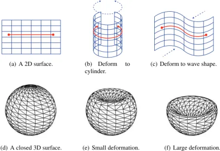
One intuitive example is that a piece of paper shown in Fig. 1(a) can be rolled up to a cylinder illustrated in Fig. 1(b) or to other curved shapes (see Fig. 1(c)). The distances between all pairs of points on the paper clearly remain the same under different shapes. Besides the open surface discussed above, similar deformation can be applied on closed surfaces (see Figs. 1(d)-1(f) for example). Clearly, ambigu-ous embeddings exist and thus a general 3D surface is not localizable under given surface distance constraints only.

(a) A 2D surface. (b) Deform to cylinder.

(c) Deform to wave shape.

(d) A closed 3D surface. (e) Small deformation. (f) Large deformation.

Fig. 1 Illustration of the non-localizability of general 3D surfaces. A surface can be deformed to

Given a wireless sensor network deployed on a 3D terrain surface with one-hop distance information available, a simple distributed algorithm introduced in (Zhou et al 2011) extracts a refined triangular mesh from the network connectivity graph. Vertices of the triangular mesh represent the set of sensor nodes. An edge between two neighboring vertices indicates the communication link between the two sensors. The state-of-the-art surafce network localization methods are based on the extracted triangular mesh structure.

Surface Network Localization with Height Information

Under a practical setting with estimated link distances (between nearby nodes) and nodal heights (i.e., Z-coordinates) obtained by measuring atmospheric pressure, a sensor network deployed on a single-value 3D surface is localizable. Briefly, a single-value surface is one on which any two points have different projections on the X-Y plane. The definition is in reference to X-Y plane since sensors’ heights are given as Z-coordinates. A planar projection of network deployed on a single-value surface converts a surface network localization problem to a planar one. The X-Y coordinates of nodes can be computed with well-known planar localization algo-rithms (Shang et al 2003; Shang and Ruml 2004; Vivekanandan and Wong 2006; Lim and Hou 2009; Jin et al 2011). The localization result is then mapped back to 3D by adding the known Z-coordinates.

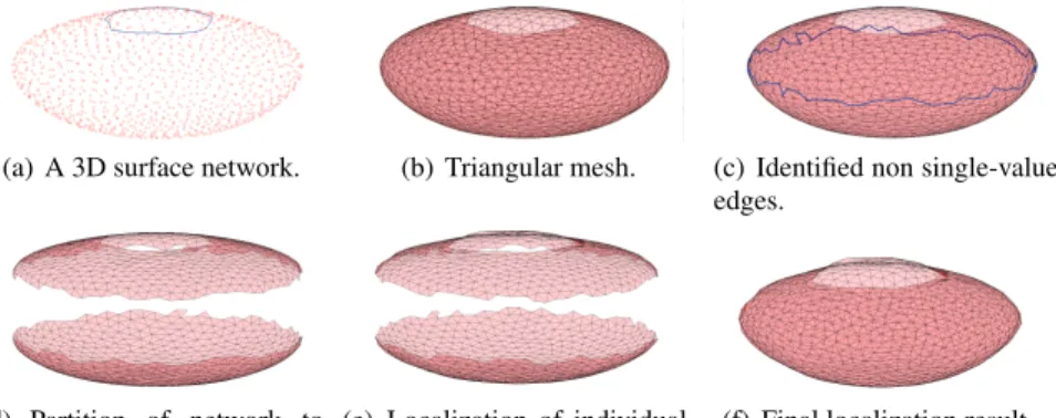
(a) A 3D surface network. (b) Triangular mesh. (c) Identified non single-value edges.

(d) Partition of network to single-value patches.

(e) Localization of individual patch.

(f) Final localization result.

Fig. 2 An overview of the cut-and-sew algorithm for general 3D surface localization.

For sensor networks deployed on general 3D surfaces, a distributed localization algorithm, dubbed cut-and-sew, applies a divide-and-conquer approach to localize sensor nodes with height informationz available. The basic idea is to partition a general 3D surface network into single-value patches, localizing individual patch and then merging them into a unified coordinates system. Note that the number

(a) (b) (c)

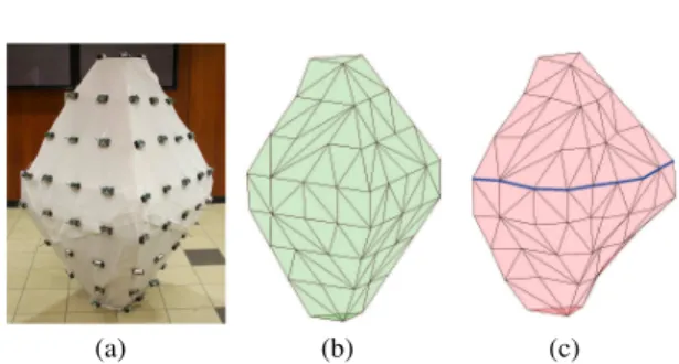
Fig. 3 Experimental setup and result. (a) Indoor 3D surface network testbed. (b) Input

triangula-tion. (c) Localization result (with an average location error of 14%).

of single-value patches should be minimized to avoid unnecessary partitioning and merging, which are subject to linear transformation errors. The key is to identify non single-value edges that guide the division of a 3D surface network into single-value patches.

Fig. 2 illustrates the basic idea of the cut-and-sew algorithm. Specifically, Figs. 2(a) and. 2(b) show a sensor network and the extracted triangular mesh, respectively. An edge is locally non single-value if the projection of its two associated triangles over-lap on the X-Y plane. Each node in the network performs a simple and localized scheme to determine whether an associated edge is a non single-value one based on its local distance information. Fig. 2(c) shows the identified non single-value edges. A set of non single-value edges form the boundary of a single-value patch. Fig. 2(d) illustrates the partition of network into a minimum set of single-value patches. Each single-value patch can then be localized as shown in Fig. 2(e). Since neighboring patches share common vertexes and edges, they can be readily “sewed” together and yield a unified coordinate system for the entire 3D surface sensor network as illustrated in Fig. 2(f).

Under practical sensor network settings, both surface distances and sensors heights are subject to measurement errors. The noisy distance and height measure-ments directly affect the identification of non single-value edges, which may devi-ate from the ground truth and become isoldevi-ated. One approach is to fuse nearby non single-value edges to form a band and then cut the network along the medial axis of the band. This method effectively minimizes the impact of input errors on network partition and localization.

Prototyping and Experiments

Fig. 3(a) shows one indoor testbed model built for prototyping 3D surface sensor networks with 5.25 feet high, 3 feet long, and 3 feet wide. Forty eight Crossbow MICAz motes are attached to its surface. The algorithmic codes are implemented in Tiny OS and run on the Crossbow sensor nodes. The sensors are configured to use close to minimum radio transmission power (Level 2) with a communication range

between 25 to 55 cm. The short radio range avoids undesired connections through volume.

Every sensor periodically broadcasts a beacon message that contains its node ID to its neighbors. Based on received beacon messages, a node builds a neighbor list with the RSSI of corresponding links. RSSI is used to estimate the length of links by looking up a RSSI-distance table established by experimental training data. The preliminary test shows that, under low transmission power, such estimation has an error rate about 20%. At the same time, the ground truth of surface distances and sensor coordinates are manually measured. Fig. 3(b) illustrates the triangulation based on ground truth inputs. Fig. 3(c) shows the localization result. The combined patches largely restore the original 3D surface network, with an average location error of about 14%.

Surface Network Localization with Digital Terrain Model

Integrating height measurement into every sensor of a network is not always prac-tical and affordable, especially for a large-scale sensor network. However, a 3D representation of a terrain’s surface, called digital terrain model (DTM), is available to public with a variable resolution up to one meter. DTMs are commonly built us-ing remote sensus-ing technology or from land surveyus-ing. A DTM is represented as a grid of squares, where the longitude, latitude, and altitude (i.e., 3D coordinates) of all grid points are known. It is straightforward to convert a grid into a triangulation, e.g., by simply connecting a diagonal of each square. Therefore a triangular mesh of a terrain surface can be available before we deploy a sensor network on it. On the other hand, a refined triangular mesh can be extracted from the connectivity graph of network deployed on the terrain surface with local distance information. The con-straint that the sensors must be on the known 3D terrain surface ensures that the triangular meshes of terrain surface and network approximate the same geometric shape. Theoretically, the two triangular meshes share the same conformal structure. We can construct a well-aligned conformal mapping between them. Based on this mapping, each sensor node of the network can easily locate reference grid points of the DTM to calculate its own location.

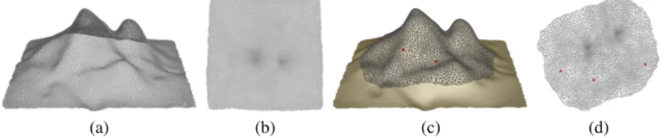
Fig. 4 illustrates the basic idea to localize a surface network on a 3D terrain surface with DTM available. Fig. 4 (a) and (c) show the triangular meshes of a ter-rain surface and a network deployed over the terter-rain surface, respectively. We first compute two conformal mappings, denoted as f1andf2respectively, to map the two

triangular meshes to plane as shown in Figs. 4 (b) and (d) respectively. However, the two mapped triangular meshes on plane are not aligned. Three anchor nodes, sen-sor nodes equipped with GPS, marked with red as shown in Fig. 4 (c) are deployed with the network to provide a reference for alignment. Based on the positions of the three anchor nodes, we construct a M ¨obius transformation, denoted as f3, to align

the mapped triangular meshes of the network and the terrain surface on plane. Com-bining the three mappings, f₁−1◦f3◦f2, induces a well-aligned conformal mapping

between the two triangular meshes shown in Fig. 4 (a) and (c), respectively. Based on the well-aligned mapping, each sensor node of the network simply locates its nearest grid points, vertices of the triangular mesh of the terrain surface, to calculate its own geographic location.

(a) (b) (c) (d)

Fig. 4 (a) The triangular mesh of a terrain surface. (b) The triangular mesh of the terrain surface

is conformally mapped to plane. (c) The triangular mesh of a network deployed on the terrain surface with three randomly deployed anchor nodes marked with red. (d) The triangular mesh of the network is conformally mapped to plane.

Deployment of Anchor Nodes

Figure 5 shows a set of representative terrain surfaces and their corresponding DTMs, on which sensor nodes marked as black points are randomly deployed. For each network, eight tests are repeated with a various deployment of three anchor nodes in each test. Table 1 shows the mean (µ), median ( ˜x), and standard devia-tion (σ) of localization errors under different deployment of anchor nodes of each network. The positions of three anchor nodes affect the performance of the local-ization algorithm slightly. In general, the more scattered the three anchor nodes are deployed in a network, the lower the localization error is.

Size of Anchor Nodes

Theoretically speaking, the localization algorithm requires only three anchor nodes to align two triangular meshes on plane, regardless of the size of a network. If more anchor nodes are deployed on the network, a least-square conformal map-ping method can replace M ¨obius transformation to incorporate all anchor nodes into the alignment to improve the localization accuracy. Fig. 6 shows one example. The localization error of a network with size 2.6k deployed on a 3D surface shown in Fig. 4(d), decreases slightly with the increased number of anchor nodes.

Table 1 The distribution of localization errors under different sets of anchor nodes

Error DTM I DTM II DTM III DTM IV

µ 0.2579 0.1356 0.0951 0.2098

˜

x 0.2306 0.1343 0.0956 0.1512

(a) DTM I (b) DTM II (c) DTM III (d) DTM IV

Fig. 5 The first row shows a set of DTMs of representative terrain surfaces. The second row shows

sensor nodes marked with black points randomly deployed on these terrain surfaces. The third row shows the localized sensor networks with anchor nodes marked with red.

3 4 5 6 7 8 9 10

The number of anchor nodes 0.07 0.075 0.08 0.085 0.09 0.095 0.1 0.105 Localization Error

Fig. 6 Localization error decreases slightly with the increased number of anchor nodes.

Applications

Geographic location information is imperative to a variety of applications in WSNs, ranging from position-aware sensing to geographic routing. While global navigation satellite systems (such as GPS) have been widely employed for localization, inte-grating a GPS receiver in every sensor of a large-scale sensor network is unrealistic due to high cost. Moreover, some application scenarios prohibit the reception of satellite signals by part or all of the sensors, rendering it impossible to solely rely on global navigation systems. In real-world applications, many large-scale WSNs are deployed over complex terrains, such as the volcano monitoring project (Werner-Allen et al 2006). The introduced state-of-the-art surface network localization

algo-rithms recover the coordinates of sensor nodes with assumption of the availability of nodal height measurements (Zhao et al 2012, 2013) or digital terrain model, a 3D representation of terrain’s surface (Yang et al 2014). They are all distributed and scalable to large-scale sensor networks deployed over general 3D terrain surfaces.

Cross-References

References

Jin M, Xia S, Wu H, Gu X (2011) Scalable and fully distributed localization with mere connectivity. In: Proc. of INFOCOM, pp 3164–3172

Lim H, Hou J (2009) Distributed localization for anisotropic sensor networks. ACM Transactions on Sensor Networks 5(2):11–37

Shang Y, Ruml W (2004) Improved mds-based localization. In: Proc. of INFOCOM, pp 2640–2651 Shang Y, Ruml W, Zhang Y, Fromherz MPJ (2003) Localization from mere connectivity. In: Proc.

of MobiHoc, pp 201–212

Vivekanandan V, Wong VWS (2006) Ordinal mds-based localization for wireless sensor networks. International Journal of Sensor Networks 1(3/4):169–178

Werner-Allen G, Lorincz K, Johnson J, Lees J, Welsh M (2006) Fidelity and yield in a volcano monitoring sensor network. In: Proceedings of the 7th symposium on Operating systems design and implementation, OSDI ’06, pp 381–396

Yang Y, Jin M, Wu H (2014) 3D Surface Localization with Terrain Model. In: Proc. of IEEE Conference on Computer Communications (INFOCOM), pp 46–54

Zhao Y, Wu H, Jin M, Xia S (2012) Localization in 3d surface sensor networks: Challenges and solutions. In: Proc. of the 31st Annual IEEE Conference on Computer Communications (IN-FOCOM’12), pp 55–63

Zhao Y, Wu H, Jin M, Yang Y, Zhou H, Xia S (2013) Cut-and-sew: A distributed autonomous localization algorithm for 3d surface wireless sensor networks. In: Proc. of the 14th ACM International Symposium on Mobile Ad Hoc Networking and Computing (MobiHoc’13) Zhou H, Wu H, Xia S, Jin M, Ding N (2011) A distributed triangulation algorithm for wireless