Continual deep learning via progressive learning

A thesis submitted in fulfilment of the requirements for the degree of Doctor of Philosophy

Haytham M. Fayek

B.Eng. (Hons), Petronas University of Technology M.Sc., Petronas University of Technology

School of Engineering

College of Science, Engineering and Health RMIT University

I certify that except where due acknowledgement has been made, the work is that of the author alone; the work has not been submitted previously, in whole or in part, to qualify for any other academic award; the content of the thesis is the result of work which has been carried out since the official commencement date of the approved research program; any editorial work, paid or unpaid, carried out by a third party is acknowledged; and, ethics procedures and guidelines have been followed.

Haytham M. Fayek Melbourne, Victoria February 4, 2019

Machine learning is one of several approaches to artificial intelligence. It allows us to build machines that can learn from experience as opposed to being explicitly programmed. Current machine learning formulations are mostly designed for learning and performing a particular task from a tabula rasa using data available for that task. For machine learning to converge to artificial intelligence, in addition to other desiderata, it must be in a state of continual learning, i.e., have the ability to be in a continuous learning process, such that when a new task is presented, the system can leverage prior knowledge from prior tasks, in learning and performing this new task, and augment the prior knowledge with the newly acquired knowledge without having a significant adverse effect on the prior knowledge. Continual learning is key to advancing machine learning and artificial intelligence.

Deep learning is a powerful general-purpose approach to machine learning that is able to solve numerous and various tasks with minimal modification. Deep learning extends machine learning, and specially neural networks, to learn multiple levels of distributed representations together with the required mapping function into a single composite function. The emergence of deep learning and neural networks as a generic approach to machine learning, coupled with their ability to learn versatile hierarchical representations, has paved the way for continual learning. The main aim of this thesis is the study and development of a structured approach to continual learning, leveraging the success of deep learning and neural networks.

This thesis studies the application of deep learning to a number of supervised learning tasks, and in particular, classification tasks in machine perception, e.g., image recognition, automatic speech recognition, and speech emotion recognition. The relation between the systems developed for these tasks is investigated to illuminate the layer-wise relevance of features in deep networks trained for these tasks via transfer learning, and these independent systems are unified into continual learning systems.

The main contribution of this thesis is the construction and formulation of a deep learning framework, denoted progressive learning, that allows a holistic and systematic approach to continual learning. Progressive learning comprises a number of procedures that address the continual learning desiderata. It is shown

that, when tasks are related, progressive learning leads to faster learning that converges to better generalization performance using less amounts of data and a smaller number of dedicated parameters, for the tasks studied in this thesis, by accumulating and leveraging knowledge learned across tasks in a continuous manner. It is envisioned that progressive learning is a step towards a fully general continual learning framework.

I am eternally grateful to all my teachers, lecturers, supervisors, and mentors. I am particularly grateful to my PhD supervisors: Professor Lawrence Cavedon and Professor Hong Ren Wu, for they have provided me the freedom to pursue my interests, were always available to provide feedback and support when needed, and were tremendously generous with their advice and mentorship.

I am thankful to Dr. Ravish Mehra and Dr. Laurens van der Maaten for hosting me at Facebook Research. My internship at Facebook was one of the highlights of this journey. I also acknowledge Associate Professor Margaret Lech for her guidance during the first year of my candidature. I am also thankful to members of the Evolutionary Computing and Machine Learning (ECML) group, collaborators, and fellow students for all the discussions and musings.

I am indebted to the Royal Melbourne Institute of Technology (RMIT) for the generous Vice-Chancellor’s PhD Scholarship (VCPS). I also acknowledge the Australian National Computing Infrastructure (NCI) and NVIDIA for the computa-tional resources. I am thankful to the School of Engineering’s administrative staff, and particularly Ms. Bethany McKinnon, for helping me navigate the university’s processes.

No words can express my gratitude to my dear parents Mohamed Fayek and Manal for their selfless devotion to my brother Hesham and myself; it is no coincidence that we both chose to pursue scholarly careers. To my late beloved grandparents, grandfather Ibrahim Elsayed and grandmother Aida Khatab, I will always cherish the values you instilled in me. To my lovely wife Agata, for her love and support.

Fayek, H. M., Cavedon, L., and Wu, H. R. (2018). On the transferability of represen-tations in neural networks between datasets and tasks. In Continual Learning Workshop, Advances in Neural Information Processing Systems (NeurIPS),

Montréal, Canada.

Fayek, H. M. (2017). MatDL: A lightweight deep learning library in MATLAB. The Journal of Open Source Software, 2(19):413.

Fayek, H. M., Lech, M., and Cavedon, L. (2017). Evaluating deep learning architectures for speech emotion recognition. Neural Networks, 92:60–68. Advances in Cognitive Engineering Using Neural Networks.

Fayek, H. M., Lech, M., and Cavedon, L. (2016b). On the correlation and transfer-ability of features between automatic speech recognition and speech emotion recognition. In Interspeech, pages 3618–3622.

Fayek, H. M., Lech, M., and Cavedon, L. (2016a). Modeling subjectiveness in emotion recognition with deep neural networks: Ensembles vs soft labels. In International Joint Conference on Neural Networks (IJCNN), pages 566–570. Fayek, H. M. (2016). A deep learning framework for hybrid linguistic-paralinguistic

speech systems. In 2nd Doctoral Consortium at Interspeech 2016, pages 1–2, Berkeley, United States.

Fayek, H. M., Lech, M., and Cavedon, L. (2015). Towards real-time speech emotion recognition using deep neural networks. InInternational Conference on Signal Processing and Communication Systems (ICSPCS), pages 1–5.

Abstract ii Acknowledgements iv List of Publications v Contents vi List of Figures ix List of Tables xv

List of Algorithms xviii

List of Abbreviations xix

List of Symbols xxi

1 Introduction 1

1.1 Artificial Intelligence and Machine Learning . . . 2

1.2 Inductive Bias and Catastrophic Forgetting . . . 4

1.3 Scope . . . 5

1.4 Contributions . . . 6

1.5 Thesis Outline . . . 7

1.6 Notation . . . 8

2 Machine Learning and Deep Learning 9 2.1 Machine Learning . . . 10 2.2 Regularization . . . 13 2.3 Optimization . . . 16 2.4 Deep Learning . . . 21 2.5 Neural Networks . . . 23 vi

2.6 Convolutional Neural Networks . . . 28

2.7 Recurrent Neural Networks . . . 30

2.8 Learning Multiple Tasks . . . 32

2.9 Continual Learning . . . 36

2.10 Summary . . . 37

3 Tabula Rasa Learning 38 3.1 Machine Perception . . . 39

3.2 Image Recognition . . . 40

3.2.1 Background . . . 40

3.2.2 Experimental Setup . . . 40

3.2.3 Results . . . 45

3.3 Automatic Speech Recognition . . . 45

3.3.1 Background . . . 46

3.3.2 Automatic Speech Recognition System . . . 47

3.3.3 Experimental Setup . . . 49

3.3.4 Results . . . 53

3.4 Speech Emotion Recognition . . . 54

3.4.1 Background . . . 54

3.4.2 Related Work . . . 55

3.4.3 Speech Emotion Recognition System . . . 56

3.4.4 Experimental Setup . . . 58

3.4.5 Results . . . 60

3.5 Discussion . . . 69

3.6 Summary . . . 69

4 Relevance of Features and Task Relatedness 71 4.1 Background . . . 72

4.2 Gradual Transfer Learning . . . 73

4.3 Experiments in Image Recognition . . . 75

4.3.1 Experimental Setup . . . 75

4.3.2 Results . . . 78

4.4 Experiments in Speech Recognition . . . 80

4.4.1 Experimental Setup . . . 80 4.4.2 Results . . . 85 4.5 Discussion . . . 89 4.6 Summary . . . 90 5 Progressive Learning 92 5.1 Background . . . 93 5.2 Related Work . . . 95

5.3 Progressive Learning . . . 97

5.3.1 Curriculum . . . 98

5.3.2 Progression . . . 99

5.3.3 Pruning . . . 101

5.4 Experiments in Image Recognition . . . 103

5.4.1 Experimental Setup . . . 103

5.4.2 Evaluation Criteria . . . 106

5.4.3 Results . . . 107

5.5 Experiments in Speech Recognition . . . 113

5.5.1 Experimental Setup . . . 115

5.5.2 Evaluation Criteria . . . 118

5.5.3 Results . . . 118

5.6 Discussion . . . 121

5.7 Summary . . . 122

6 Conclusions and Future Work 124 6.1 Conclusions . . . 125 6.2 Future Work . . . 126 Bibliography 128 A Datasets 146 A.1 CIFAR . . . 146 A.2 eNTERFACE . . . 149 A.3 IEMOCAP . . . 149 A.4 ImageNet . . . 149 A.5 SVHN . . . 150 A.6 TIMIT . . . 150

1.1 Conceptual taxonomy of artificial intelligence, continual learning, classical machine learning, representation learning, and deep learning. Note that this taxonomy does not imply that all classical machine learning, representation learning, and deep learning methods are continual learning methods. . . 3

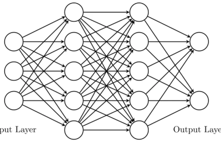
2.1 Dropout. Left. A complete fully connected neural network with one hidden layer. Right. The same fully connected neural network with a number of omitted units. . . 16

2.2 Feed-forward fully connected neural network with two hidden layers. 23

2.3 Non-linear activation functions. Left. Logistic sigmoid function. Centre. Hyperbolic tangent function. Right. Rectified linear unit. 25

2.4 Convolutional neural network with three Convolutional (Conv) and Pooling (Pool) layers followed by a Fully Connected (FC) layer. . . 29

2.5 Recurrent neural network with two recurrent hidden layers charac-terized by self-connections (blue). . . 30

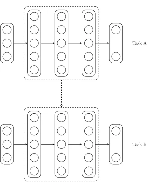
2.6 Transfer learning via a neural network with three hidden layers. Top. The parameters of the model were randomly initialized, and trained for Task A. Bottom. The parameters of the model were initialized using the parameters trained for Task A, and fine-tuned for Task B. . . 34

2.7 Multi-task learning with three tasks via a neural network that has three hidden layers. All layers are shared between the three tasks except the output layer which is unique to each task. . . 35

3.1 Acoustic speech signal. Top. Raw acoustic signal in the time do-main. Centre. Normalizedlog Mel Frequency Spectral Coefficients

(MFSCs) computed from the raw acoustic signal (top). Bottom. Normalized Mel Scale Cepstral Coefficients (MFCCs) computed from the raw acoustic signal (top). . . 48

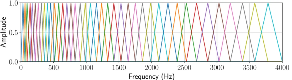
3.2 Mel scale filter banks. The amplitudes of 40 filter banks on a Mel

scale in the frequency range 0–4 kHz. . . 49

3.3 Overview of the proposed speech emotion recognition system. A deep multi-layered neural network, composed of several fully connected, convolutional, or recurrent layers, ingests a target frame (solid), concatenated with a number of context frames (dashed), to predict the probabilities over emotion classes corresponding to the target frame. . . 57

3.4 Speech emotion recognition test accuracy and test Unweighted Av-erage Recall (UAR) on the IEMOCAP dataset with a deep neural network as a function of the number of context frames. . . 61

3.5 Speech emotion recognition test accuracy on the IEMOCAP dataset of a Long Short-Term Memory (LSTM)-Recurrent Neural Network (RNN) with various number of context frames. LSTM-RNN-c

de-notes the sequence length which the model was trained on. The number of frames denotes the sequence length which the model was evaluated on. . . 64

3.6 Speech emotion recognition test Unweighted Average Recall (UAR) on the IEMOCAP dataset of a Long Short-Term Memory (LSTM)-Recurrent Neural Network (RNN) with various number of context frames. LSTM-RNN-c denotes the sequence length which the model was trained on. The number of frames denotes the sequence length which the model was evaluated on. . . 65

3.7 Input speech utterances (top) and corresponding aligned output (below) of the speech emotion recognition system for a number of selected utterances from the test subset of the IEMOCAP dataset. The output is the probabilities over classes denoting the confidence of the model. Transcripts: (a): Oh, laugh at me all you like but why does this happen every night she comes back? She goes to sleep in his room and his memorial breaks in pieces. Look at it, Joe look. (Angry); (b): I will never forgive you. All I’d done was sit around wondering if I was crazy waiting so long, wondering if you were thinking about me. (Happy); (c): OKay. So I am putting out the pets, getting the car our the garage. (Neutral); (d): They didn’t die. They killed themselves for each other. I mean that, exactly. Just a little more selfish and they would all be here today. (Sad); (e): Oh yeah, that would be. Well, depends on what type of car you had, though too. I guess it would be worth it. helicopter. Yeah, helicopter. There is a helipad there, right? Yeah, exactly. (Happy). 67

4.1 Gradual transfer learning between two tasks. The parameters of the first and second models are initialized randomly (grey) and trained for Task A (blue) and Task B (green) respectively. The third and fourth models are examples of gradual transfer learning. The parameters of the third model are initialized using the trained Task A model (blue) and the final three layers are fine-tuned for Task B (green). The parameters of the fourth model are initialized using the trained Task B model (green) and all layers except the first layer are fine-tuned for Task A (blue). . . 74

4.2 Gradual transfer learning between the CIFAR-10 and CIFAR-100 datasets. Left. The validation and test accuracies of indepen-dent CIFAR-10 (dashed) and CIFAR-10 fine-tuned from CIFAR-100 (solid) as a function of the number of constant layers. Right. The validation and test accuracies of independent CIFAR-100 (dashed) and CIFAR-100 fine-tuned from CIFAR-10 (solid) as a function of the number of constant layers. . . 79

4.3 Gradual transfer learning between the CIFAR-10 and SVHN datasets. Left. The validation and test accuracies of independent CIFAR-10 (dashed) and CIFAR-10 fine-tuned from SVHN (solid) as a function of the number of constant layers. Right. The validation and test accuracies of independent SVHN (dashed) and SVHN fine-tuned from CIFAR-10 (solid) as a function of the number of constant layers. 79

4.4 Gradual transfer learning between the CIFAR-100 and SVHN datasets. Left. The validation and test accuracies of independent CIFAR-100 (dashed) and CIFAR-100 fine-tuned from SVHN (solid) as a function of the number of constant layers. Right. The validation and test accuracies of independent SVHN (dashed) and SVHN fine-tuned from CIFAR-100 (solid) as a function of the number of constant layers. 80

4.5 Learned features in the first layer of the convolutional neural network Model A detailed in Table 4.3 for the automatic speech recognition task (left) and the speech emotion recognition task (right). . . 86

4.6 Gradual transfer learning between the automatic speech recognition task and the speech emotion recognition task with convolutional neural network Model A. Left. The Phone Error Rate (PER) of independent automatic speech recognition (TIMIT) (dashed) and automatic speech recognition (TIMIT) fine-tuned from speech emo-tion recogniemo-tion (IEMOCAP) (solid) as a funcemo-tion of the number of constant layers. Right. The Unweighted Error (UE) of indepen-dent speech emotion recognition (IEMOCAP) (dashed) and speech emotion recognition (IEMOCAP) fine-tuned from automatic speech recognition (TIMIT) (solid) as a function of the number of constant layers. . . 87

4.7 Gradual transfer learning between the automatic speech recognition task and the speech emotion recognition task with convolutional neural network Model B. Left. The Phone Error Rate (PER) of independent automatic speech recognition (TIMIT) (dashed) and automatic speech recognition (TIMIT) fine-tuned from speech emo-tion recogniemo-tion (IEMOCAP) (solid) as a funcemo-tion of the number of constant layers. Right. The Unweighted Error (UE) of indepen-dent speech emotion recognition (IEMOCAP) (dashed) and speech emotion recognition (IEMOCAP) fine-tuned from automatic speech recognition (TIMIT) (solid) as a function of the number of constant layers. . . 88

5.1 Overview of progressive learning for three tasks. Initially, a curricu-lum strategy is used to select a task (blue) from the pool of candidate tasks. Second, a model is trained to perform the selected task (blue), and the learned parameters are constant thereafter. Third, the cur-riculum strategy is employed to select the subsequent task (purple). Fourth, new model parameters, denoted progressive block, which draw connections from the preceding layer in the block as well as the preceding layer in prior progressive block(s), are added and trained to perform the selected task (purple). Fifth, after training the newly added progressive block to convergence, a pruning procedure is used to remove weights without compromising performance. Finally, the curriculum, progression, and pruning procedures are repeated for the third task (green), and for all remaining task(s) subsequently. . 94

5.2 Procedural illustration of progressive learning for three tasks. In the first iteration, a curriculum strategy is used to select a task (blue) from the pool of candidate tasks. Then, a model is trained to perform the selected task (blue), and the learned parameters are constant thereafter. In the second iteration, the curriculum strategy is employed to select the subsequent task (purple). Then, new model parameters, denoted progressive block, which draw connections from the preceding layer in the block as well as the preceding layer in prior progressive block(s), are added and trained to perform the selected task (purple). Subsequently, after training the newly added progressive block to convergence, a pruning procedure is used to remove weights without compromising performance. In the third iteration, the curriculum, progression, and pruning procedures are repeated for the third task (green). Further iterations of the three procedures continue for all following task(s). . . 97

5.3 Illustration of the concatenation operation for three blocks. . . 101

5.4 Accuracy of progressive learning vs. independent learning for all 11

image recognition tasks. The tasks are ordered according to the outcome of the curriculum procedure. C-10 denotes the CIFAR-10 task, C-100-s indicates the sth _{CIFAR-100 task. . . . 110}

5.5 Learning curves, validation error as a function of training iterations, for progressive and independent learning for the 11CIFAR-10 and

CIFAR-100 tasks. Progressive Learning demonstrates faster learning compared with independent learning. Note that tasks are ordered according to the outcome of the curriculum strategy. Models are reset to random initialization at the beginning of each task in the case of independent learning. . . 112

5.6 Total number of parameters in the model as a function of tasks. Left. The total number of parameters in the model as a function of tasks before and after pruning. Centre. The number of fixed parameters (parameters in preceding progressive blocks) as a function of tasks before and after pruning. Right. The number of adaptive parameters (parameters in the progressive block being trained) as a function of tasks before and after pruning. . . 113

5.7 Percentage of pruned weights as a function of layers. It can be noted that initial layers are more prone to pruning as progressive blocks can rely on features learned in initial layers in prior progressive blocks.114

5.8 Progressive learning vs independent learning for all four speech recognition tasks. The tasks are ordered according to the outcome of the curriculum procedure. . . 119

5.9 Learning curves, validation error as a function of training iterations, for progressive and independent learning for the four speech recogni-tion tasks. Note that tasks are ordered according to the outcome of the curriculum strategy. Models are reset to random initialization at the beginning of each task in the case of independent learning. . 120

A.1 Sample images randomly drawn from the training set of the CIFAR-10 dataset. Each row was drawn from a single class in the following order: airplane, automobile, bird, cat, deer, dog, frog, horse, ship, and truck. . . 148 A.2 Sample images randomly drawn from the training set of the SVHN

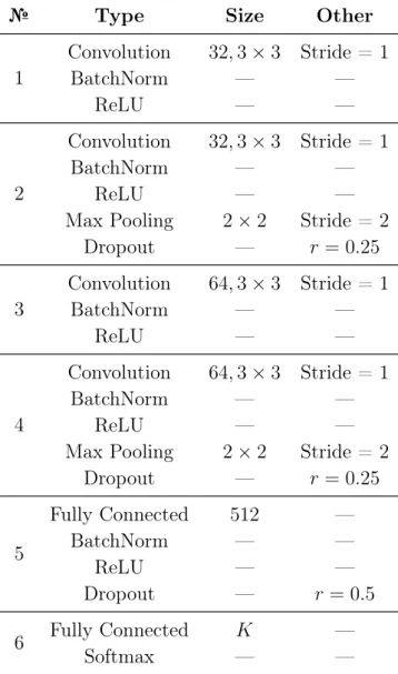
3.1 Convolutional neural network Model A architecture for the image recognition task. K denotes the number of output classes. . . 43

3.2 Densely connected convolutional network Model B architecture for the image recognition task. The outputs of the convolutional layers in Blocks 2, 4, and 6, are concatenated with the inputs to the layer and fed to the subsequent layer in the same block. K denotes the

number of output classes. . . 44

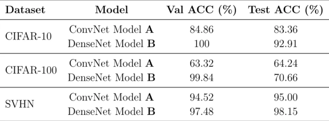
3.3 Image recognition Validation Classification Accuracy (Val ACC) and Test Classification Accuracy (Test ACC) on the CIFAR-10, CIFAR-100, and SVHN datasets. . . 46

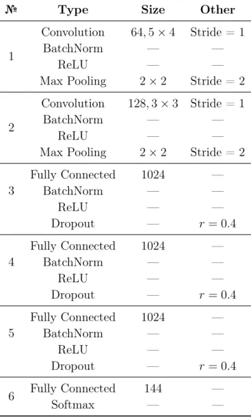
3.4 Convolutional neural network Model A architecture for the auto-matic speech recognition task. . . 51

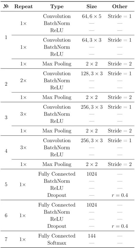
3.5 Convolutional neural network ModelBarchitecture for the automatic speech recognition task. . . 52

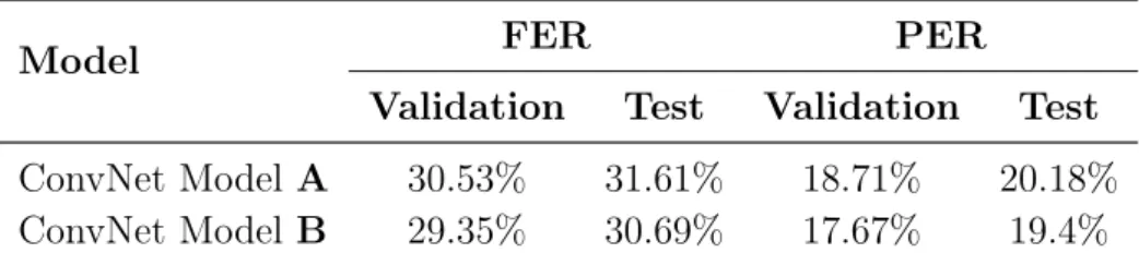
3.6 Automatic speech recognition validation and test Frame Error Rate (FER) and Phone Error Rate (PER) on the TIMIT dataset. . . 54

3.7 Speech emotion recognition test Accuracy (ACC) and test Un-weighted Average Recall (UAR) on the IEMOCAP dataset with various convolutional neural network architectures. Conv(c_×j_×k)

and Conv1D(c×j×k) denote a spatial convolutional layer and a

temporal convolutional layer respectively ofcfilters, each of sizej_×k,

with stride 2, followed by Batch Normalization (BatchNorm) and

Rectified Linear Units (ReLUs). FC(nl) denotes a fully connected

layer ofnl units followed by BatchNorm, ReLUs, and dropout. All

architectures have a fully connected layer with a softmax function as the output layer. . . 62

3.8 Speech emotion recognition test Accuracy (ACC) and Unweighted Average Recall (UAR) on the IEMOCAP dataset with various neural network architectures. Conv(c_×j _×k) denote a spatial

convolu-tional layer ofcfilters, each of size j_×k, with stride 2, followed by

Batch Normalization (BatchNorm) and Rectified Linear Units (Re-LUs). FC(nl) denotes a fully connected layer of nl units followed by

BatchNorm, ReLUs, and dropout. LSTM-RNN(nl) denotes a Long

Short-Term Memory (LSTM)-Recurrent Neural Network (RNN) of

nlunits. All architectures have a fully connected layer with a softmax

function as the output layer. . . 66

3.9 Speech Emotion Recognition (SER) results reported in prior work on the IEMOCAP dataset. Note that differences in data subsets and other experiment conditions should be taken into consideration when comparing the following results against each other, see references for more details. . . 68

4.1 Densely connected convolutional network architecture for image recognition. The outputs of the convolutional layers in Blocks 2, 4, and 6, are concatenated with the inputs to the layer and fed to the subsequent layer in the same block. K denotes the number of

output classes. . . 76

4.2 Speech recognition convolutional neural network Model A architec-ture. K denotes the number of output classes. . . 83

4.3 Speech recognition convolutional neural network Model B architec-ture. K denotes the number of output classes. . . 84

4.4 Validation and test Frame Error Rate (FER) and Phone Error Rate (PER) of gradual transfer learning from the speech emotion recognition task (IEMOCAP) to the automatic speech recognition task (TIMIT) with convolutional neural network Model A. . . 86

4.5 Validation and test error and unweighted error of gradual transfer learning from the automatic speech recognition task (TIMIT) to the speech emotion recognition task (IEMOCAP) with convolutional neural network Model A. . . 87

4.6 Validation and test Frame Error Rate (FER) and Phone Error Rate (PER) of gradual transfer learning from the speech emotion recognition task (IEMOCAP) to the automatic speech recognition task (TIMIT) with convolutional neural network Model B. . . 88

4.7 Validation and test error and unweighted error of gradual transfer learning from the automatic speech recognition task (TIMIT) to the speech emotion recognition task (IEMOCAP) with convolutional neural network Model B. . . 89

5.1 Convolutional neural network architecture for the image recognition tasks. The concatenation operation indicates the layers at which the output of the previous layer in all prior blocks are concatenated. The concatenation operation can be ignored in independent learning.105

5.2 Progressive learning Validation Average Accuracy (Val AA) and Test Average Accuracy (Test AA) over all 11tasks using the CIFAR-10

and CIFAR-100 datasets unless otherwise indicated. . . 108

5.3 Progressive learning Validation Progressive Knowledge Transfer (Val PKT) and Test Progressive Knowledge Transfer (Test PKT) over all 11 tasks using the CIFAR-10 and CIFAR-100 datasets unless

otherwise indicated. . . 109

5.4 Convolutional neural network architecture for the speech recognition tasks. The concatenation operation indicates the layers at which the output of the previous layer in all prior blocks are concatenated. The concatenation operation can be ignored in independent learning.

K denotes the number of output classes. . . 117

2.1 Early stopping algorithm for determining when to terminate an iterative training algorithm. . . 15

2.2 Stochastic gradient descent algorithm. Note that supervised learning is assumed herein, but the algorithm is valid for other types of learning that can provide means to compute the gradients. . . 18

2.3 Adam algorithm. is a small constant for numerical stability (e.g., = 10−8). The division and square root in Step 10 are applied element-wise. . . 20

2.4 Forward propagation through a fully connected (deep) neural net-work. φ denotes a non-linear operation applied element-wise. Note

that for notational convenience, the output of the output layer in the network yˆ(L) is abbreviated to yˆ. The algorithm assumes a single

exemplar m but can be extended to the case with a mini-batch of

exemplars or the entire dataset. . . 27

2.5 Backward computation through a fully connected (deep) neural net-work. φ0 _{denotes the derivative of the non-linear operation applied}

element-wise. denotes the Hadamard product. > denotes the transpose operation. λ is the regularization weight and the entire

term can be ignored if the loss function does not constitute a reg-ularization penalty Ω. Note that for notational convenience, the

output of the output layer in the networkyˆ(L) is abbreviated to yˆ.

The algorithm assumes a single exemplar m but can be extended to

the case with a mini-batch of exemplars or the entire dataset. . . . 28

5.6 Functional decomposition of progressive learning in the supervised learning case. . . 99

5.7 Greedy layer-wise pruning procedure in progressive learning. . . 103

AI Artificial Intelligence. ANN Artificial Neural Network. ASR Automatic Speech Recognition. BatchNorm Batch Normalization.

BPTT BackPropagation Through Time. ConvNet Convolutional Neural Network. CPU Central Processing Unit. DCT Discrete Cosine Transform.

DenseNet Densely Connected Convolutional Network. DFT Discrete Fourier Transform.

DNN Deep Neural Network. ELM Extreme Learning Machine. ERM Empirical Risk Minimization. FER Frame Error Rate.

GMM Gaussian Mixture Model. GPU Graphics Processing Unit. GR Gender Recognition. HMM Hidden Markov Model.

HOG Histograms of Oriented Gradient.

IID Independent and Identically Distributed.

LOSO Leave-One-Speaker-Out. LSTM Long Short-Term Memory. MAP Maximum A Priori.

MFCC Mel Frequency Cepstral Coefficient. MFSC Mel Frequency Spectral Coefficient. MLE Maximum Likelihood Estimation. MLP Multi-Layer Perceptron.

MSE Mean Squared Error. NN Neural Network.

PCA Principal Component Analysis. PER Phone Error Rate.

RBM Restricted Boltzmann Machine. ReLU Rectified Linear Unit.

ResNet Residual Network.

RNN Recurrent Neural Network. SER Speech Emotion Recognition. SGD Stochastic Gradient Descent. SIFT Scale Invariant Feature Transform. SR Speaker Recognition.

SVM Support Vector Machine. UAR Unweighted Average Recall. UE Unweighted Error.

x Scalar.

X Constant.

x Vector.

X Matrix or Tensor. X Set or Special Notation.

X Set or Special Notation. xi Element i of Vectorx.

Xi Element i of Set X.

Xij Element in Row i and Column j of MatrixX.

Xi: Element(s) in Row i of MatrixX.

p(i) Probability Distribution Over i.

p(i|j) Conditional Probability Distribution Over i Givenj. p(i|j;θ) p(i|j) Parametrized by Parameters θ. f _{Concatenation Operation.} ∗ Convolution Operation. E Expectation. ∇i Gradient of i. Hadamard Product. Small Constant. > Transpose Operation. ki_kj Lj Norm of i.

sigm Logistic Sigmoid Function.

tanh Hyperbolic Tangent Function.

R Set of Real Numbers. D Dataset.

Θ Parameter Space.

θ Vector of All Adaptive Parameters in a Model.

W Matrix of Weights.

W(i) Matrix of Weights of layer i.

b Vector of Biases.

L Number of Layers in a Deep Network.

Introduction

A

Ma-chine learning is one of several approaches to artificial intelligence. It allows us to build machines that can learn from experience as opposed to being explicitly programmed. Current machine learning algorithms and methodologies are mostly designed for learning and performing a particular task from a tabula rasa using data available for the task at hand. For machine learning to converge to artificial intelligence, in addition to other desiderata, it must be in a state of continual learning, i.e., have the ability to be in a continuous learning process, such that when a new task is presented, it can leverage prior knowledge from prior tasks, in learning and performing this new task, and augment the prior knowledge with the newly acquired knowledge without having a significant adverse effect on the prior knowledge. Continual learning is key to advancing machine learning and artificial intelligence.

Outline. This chapter is structured as follows. Section 1.1 provides a brief introduction to artificial intelligence, machine learning, and continual learning.

Section 1.2 describes the problem statement which this work is set to address.

Section 1.3 outlines the scope of this work. Section 1.4 lists the contributions of this thesis. Section 1.5 details the thesis outline. Finally,Section 1.6 summarizes the notation used throughout the thesis.

1.1

Artificial Intelligence and

Machine Learning

Artificial Intelligence (AI) aims to understand and build intelligent entities∗_. Con-temporary AI has been sought after ever since the inception of the first pro-grammable digital computer [Turing, 1950]. Nonetheless, the seeds of AI were planted long before that, and can be traced to antiquity, when humans devised and solicited statues and automatons depicting gods for wisdom and emotion [ McCor-duck, 2004]. Later, classical philosophers delineated formal processes for logical reasoning, e.g., Aristotelian syllogism, which was built on the notion that human thought could be mechanized. This notion is one of the main assumptions in many approaches to AI[Russell and Norvig, 2003], and can be conceived using mathe-matical logic [Boole, 1854] implemented using programmable digital computers. Progress in the field of AI has been swift relative to its young age [McCorduck et al., 1977]. Today, there are many approaches to AI, such as symbolic reasoning and computational intelligence, that may one day lead to thinking machines that have intellectual capabilities superior to those of humans. Theoretically, thinking machines are only limited by the limits of computation and physics [Schmidhuber, 2002].

Machine learning is one of several approaches toAI. Notably, it is able to deal with tasks that are easy for humans to perform but hard for them to formalize how it was performed [Goodfellow et al., 2016], such as recognizing and converting speech into text, assessing visual aesthetics, or driving a car. Each of these tasks cannot be defined by a complete set of formal rules, and therefore programming machines to directly perform such tasks would result in error-prone, fragile, or incomplete programs. Machine learning allows machines to learn from experience as opposed to being explicitly programmed [Samuel, 1959]. Machine learning can be formally defined as follows: “A computer program is said to learn from experienceE

with respect to some class of tasksT and performance measureP, if its performance

at tasks inT, as measured by P, improves with experience E” [Mitchell, 1997].

The machine learning approach relies on data to learn a model that can be used to accomplish the required task [Bishop, 1995]. This encompasses engineering a data representation, choosing an architecture for the model, deriving an appropriate loss function†, and selecting a suitable training algorithm. Such decisions require domain knowledge and are naturally heuristic. Engineering a representation of the data, which is known asfeature engineering, is especially challenging, as it is difficult to determine which features should be used in advance for a particular problem;

∗_{See [Russell and Norvig, 2003] for formal definitions ofAI.}

†_{The loss function is also known as cost function, error function, fitness function, or objective}

Deep

Learning RepresentationLearning

Classical Machine Learning

Continual

Learning IntelligenceArtificial

Figure 1.1: Conceptual taxonomy of artificial intelligence, continual learning, classical machine learning, representation learning, and deep learning. Note that this taxonomy does not imply that all classical machine learning, representation learning, and deep learning methods are continual learning methods.

with a poor choice of features, all subsequent effort can be futile [Mitchell, 1997]. Representation learning alleviates the dependence of machine learning on feature engineering by learning appropriate representations for the required task [Bengio

et al., 2013]. Deep learning extends representation learning to learn multiple

levels of representations together with the mapping function, be it classification or regression or otherwise, into a single composite function.

Deep learning is, therefore, an approach to machine learning (see Figure 1.1). It allows learning representations and concepts in a hierarchical way. This can be achieved by decomposing computational models or graphs into multiple layers of processing, with the aim of learning representations of the data with multiple levels of abstraction [LeCun et al., 2015]. In doing so, the model can adaptively learn low-level features from raw data and higher-level features from the low-level features in a hierarchical manner [Hinton et al., 2006]. Notably, deep learning presents itself as a general-purpose approach to machine learning that is able to solve numerous and various tasks with minimal modification. At present, deep learning is the state-of-the-art approach to machine learning, and is prominent in numerous fields, such ascomputer vision, speech recognition, and natural language processing.

Neural networks are a class of machine learning systems‡ [Rosenblatt, 1958,

Rumelhart and McClelland, 1986]. A neural network is a collection of nodes or

units that are inter-connected via adaptive weights to form a directed weighted ‡_{Artificial Neural Networks (ANNs)are also referred to asMulti-Layer Perceptrons (MLPs).}

graph, which can learn distributed representations and ultimately the task at hand.

A Deep Neural Network (DNN), a neural network with many hierarchical layers, is

the most prevalent example of deep learning, where one layer feeds the subsequent layer, such that initial layers learn simple features from the data and subsequent layers learn more complex features using the simple features in initial layers.

Learning from a tabula rasa is the most common machine learning paradigm [Mikolov et al., 2018,Lake et al., 2017]. For an arbitrary task, a model is initialized and trained using a dataset or environment to achieve a certain objective. Contrary to human learning, the model does not typically take into account knowledge learned in prior related tasks that used prior datasets or environments, which could lead to a slower learning process that requires more data and possibly suboptimal performance [Lake et al., 2017].

For machine learning to converge to AI, in addition to other desiderata, it must be in a state ofcontinual learning [Thrun and Mitchell, 1995,Mitchell et al.,

2018], i.e., have the ability to be in a continuous learning process, such that when a new task is presented, it can leverage prior knowledge from prior tasks, in learning and performing this new task, and augment the prior knowledge with the newly acquired knowledge without having a significant adverse effect on the prior knowledge. Quintessentially, humans are always in a state of continual learning [Harlow, 1949,Smith et al., 2002,Dewar and Xu, 2010]. For instance, when presented with the task of learning a new language, one will automatically draw from one’s own past experiences with languages they are familiar with, to facilitate the learning of this new language, e.g., English speakers would naturally use their knowledge of the English syntax when learning French.

Within machine learning, deep learning and neural networks are particularly suited for continual learning, due to their unprecedented success in numerous and various tasks with minimal modification and their innate ability to learn multiple hierarchical levels of versatile distributed representations. For example, a unit in a neural network that has learned the concept of a wheel in a bicycle detection task can be used in learning to detect cars in a self-driving car task, which avoids the need to re-learn the concept of the wheel.

Continual learning is key to advancing machine learning and AI, where knowl-edge can be accumulated, repurposed, and reused over tasks.

1.2

Inductive Bias and Catastrophic Forgetting

Every machine learning algorithm with the ability to generalize beyond the data which it has encountered during training has, by definition, some form of prior, known asinductive bias [Mitchell, 1980]. Inductive bias is the set of assumptions that the model relies on to generalize beyond the data it has not encountered

during training. For example, linear regression assumes that the relation between the independent variables (input) and dependent variables (output) is linear.

Ideally, one aspires to minimize the inductive bias in a machine learning al-gorithm. There is, however, a trade-off between the inductive bias of an algo-rithm and the amount of data required to ensure reliablegeneralization to unseen data [Mitchell, 1980,Baxter, 2000], in that the search space for a solution needs to be large enough to contain a solution to the task, and small enough to not require a large dataset to navigate the search space during training. Revisiting the previous example regarding linear regression, by assuming that the relation between the independent variables and dependent variables is linear, all non-linear solutions are effectively eliminated from the search space; the search space is simpler yet may not contain the solution to the task if a non-linear solution is necessary.

Deep learning and neural networks require large datasets to learn a given task due to the large search space inherent in their design. Inductive bias can play an important role in navigating this large search space during training, and thus, alleviate the requirement of large datasets which typically leads to a slower learning process.

Continual learning is in itself a form of inductive bias. However, it can be considered a soft form of inductive bias, whereby the model can rely on existing solutions to related tasks in its search for a solution in the search space, or use data available for the task at hand to navigate the search space, or both. In doing so, one can expect a faster learning process and better generalization, using less amounts of data.

It can be seen how continual learning can be used as a form of inductive bias to improve the learning and execution of new tasks given prior related tasks; however, this should not be at the expense of corrupting the solutions to prior tasks.

Catastrophic forgetting in machine learning is the tendency to forget previously learned information when learning new information [McCloskey and Cohen, 1989,

Ratcliff, 1990]. Catastrophic forgetting is evident in parametric machine learning algorithms, where parameters learned for old task(s) are repurposed for the new task at hand, and the model forgets the old task(s) as the parameters move in the search space during the training phase for the new task.

Inducing the correct inductive bias and mitigating catastrophic forgetting in an efficient manner are two of the main challenges in continual learning.

1.3

Scope

Continual learning applies to all branches of machine learning, includingsupervised learning, unsupervised learning, and reinforcement learning§. The focus of this

work lies at the intersection between continual learning and deep learning. The class of tasks studied in this work are all cast as supervised learning problems, and in particular, classification tasks in the image recognition and speech recognition domains, both of which are sub-domains of machine perception. Nevertheless, the propositions and conclusions put forward herein are not confined to such learning tasks, and are envisaged to be applicable to other branches of machine learning, particularly those that utilize deep learning.

1.4

Contributions

The contributions of the thesis are as follows.

• The application of deep learning requires a plethora of design decisions and ex-tensive tuning of hyperparameters to ensure good performance, e.g., choosing the architecture of the neural network, including the number of layers and size of each layer. These design decisions and hyperparameters are cumbersome and are usually task-specific or domain-specific. It is therefore advantageous to understand some of these design decisions and hyperparameters across a variety of tasks. To this end, various tasks, namely, image recognition,

Automatic Speech Recognition (ASR), and Speech Emotion Recognition

(SER), were formulated and studied in a systematic manner. The SER task

was comprehensively considered and used as a test bed to explore various neural network architectures as the task itself can be formulated in multi-ple ways. This is the first empirical exploration of various deep learning formulations and architectures applied to SER. Empirical analysis provided intuition and insights on the effectiveness of some of these architectures and their suitability to particular tasks. As a consequent result of the systematic exploration, state-of-the-art results were reported on the Interactive Emo-tional Dyadic Motion Capture (IEMOCAP) dataset [Busso et al., 2008] for speaker-independentSER¶_.

• In order to move from single-task systems to systems that aim to address multiple tasks, one ought to understand the relation between these tasks. A methodology for understanding the relation between two tasks using the features learned for each task in a deep network is proposed in this work, to illuminate the relevance of each layer of features in the multi-layered neural network trained for one task to the other task via transfer learning. Understanding the layer-wise transferability of features and task relatedness is envisaged to be valuable in designing and implementing systems that ¶_{Compared to prior literature when the work was published in [Fayek et al., 2017].}

aim to address multiple tasks, by taking into consideration the overlap between closely related tasks as well as the interference between non-related or adversary tasks.

• Continual learning is a machine learning paradigm, whereby tasks are learned in sequence with the ability to use prior knowledge from previously learned tasks to facilitate the learning and execution of new ones. The main contribu-tion of this work is the construccontribu-tion and formulacontribu-tion of a novel deep learning framework, named progressive learning, that allows a holistic and systematic approach to continual learning. Progressive learning comprises a number of procedures that address the continual learning desiderata. It is shown that, when tasks are related, progressive learning leads to faster learning that converges to better generalization performance using less amounts of data and a smaller number of dedicated parameters, for the tasks studied in this thesis, by accumulating and leveraging knowledge learned across tasks in a continuous manner.

The above three contributions are put forward in Chapters 3, 4 and5 respec-tively‖_.

1.5

Thesis Outline

The thesis is structured as follows.

Chapter 1 presents a brief introduction to AI, machine learning, and continual learning, and an outlook on the state-of-the-art; provides the problem statement which this thesis is set to address; defines the scope and highlights contributions of this work, as well as the thesis outline and notation used.

Chapter 2 reviews machine learning, deep learning, and continual learning. The

concepts, theory, and mathematical framework that constitute the foundations of this work are detailed therein.

Chapter 3 builds understanding, insights, and baselines of the various tasks

used throughout this work, as well as datasets, deep learning architectures, and best practices. The SERtask is comprehensively considered and used as a test bed ‖_{An additional contribution is the development and release of an open-source lightweight}

deep learning library, calledMatDL[Fayek, 2017]. MatDL was developed natively in_Matlab and implements some commonly used deep learning building blocks and algorithms. MatDL is convenient in cases where_Matlabis preferred, or if it is required to be closely linked with other libraries written in_Matlabor Octave. MatDL is ideal for rapid machine learning research and experimentation, specially with small or medium-sized datasets, as it was designed with an emphasis on modularity, flexibility, and extensibility.

to explore various neural network architectures. The work presented in this chapter is based on [Fayek et al., 2015,Fayek et al., 2016a,Fayek et al., 2017,Fayek, 2017].

Chapter 4 is an investigation into the specificity and transferability of learned features in deep networks across multiple tasks, and how this can be used to understand task relatedness. The aim of this chapter is to gain intuition into how information propagates in deep networks that can be used to build systems with multiple tasks. The work presented in this chapter is based on [Fayek, 2016,Fayek et al., 2016b,Fayek et al., 2018].

Chapter 5 builds on work carried out in the previous two chapters and proposes

progressive learning, a novel deep learning framework that formulates continual learning into three procedures: curriculum,progression, and pruning. Progressive learning is evaluated on a number of tasks in the image recognition and speech recognition domains that were studied in the previous chapters to demonstrate its advantages compared with baseline methods.

Chapter 6 concludes the thesis and highlights avenues for future work.

1.6

Notation

The following notation is used throughout this thesis unless otherwise specified. Standard weight lower-case letters (e.g., x) are used to denote scalars. Standard

weight upper-case letters (e.g., X) are used to denote constant scalars. Boldface

lower-case letters (e.g., x) are used to denote vectors. Boldface upper-case letters (e.g., X) are used to denote matrices or tensors. Standard weight upper-case calligraphic or open-face letters (e.g., X or X) are used to denote sets and special

notation.

Single subscripts are used to denote an element in a vector or set (e.g., x_i or Xi). Double (or triple or more, depending on the order) subscripts are used to

denote an element or elements in a matrix or tensor (e.g., Xij or Xijk), where the

symbol “:” may be used to denote the entire row, or column, or dimension (e.g.,X_i: for rowi in matrix X). Single superscripts or subscripts in parentheses are used to differentiate variables (e.g., W(i) can refer to the matrix of weights of layer i).

Machine Learning and

Deep Learning

M

is said to learn from experience E with respect to some class of tasks T

and performance measure P, if its performance at tasks in T, as measured by P, improves with experience E” [Mitchell, 1997]. Following this definition, the

concepts, theory, and mathematical framework that constitute the foundations of this work are detailed in this chapter, including statistical machine learning, regularization, optimization, deep learning, neural networks, learning multiple tasks, and continual learning.

Outline. This chapter is structured as follows. Section 2.1 provides the assump-tions, theory, formulation, and mathematical framework of statistical machine learning. Section 2.2 presents popular regularization techniques for improving the generalization of machine learning models. Section 2.3 describes gradient-based optimization algorithms relevant to training neural networks. Section 2.4 presents the motivation, background, and fundamentals of deep learning. Section 2.5 is an exposition of feed-forward fully connected neural networks. Section 2.6 presents convolutional neural networks. Section 2.7 describes recurrent and long short-term memory neural networks. Section 2.8 outlines machine learning paradigms that incorporate learning multiple tasks. Section 2.9introduces continual learning and reviews selected prior literature. Finally,Section 2.10 summarizes the chapter.

2.1

Machine Learning

Machine learning can be broadly classified into supervised learning, reinforcement learning, and unsupervised learning [Bishop, 2006,Russell and Norvig, 2003,Barber, 2012]. Supervised learning relies on labels or targets in labelled datasets for the training signal during the training phase. Reinforcement learning uses a reward function, that can provide positive or negative values to indicate desired or undesired outcomes, often associated with actions, to obtain the training signal during the training phase. Unsupervised learning does not require extra information, such as labels, targets, or a reward function, for the training signal. Other classifications may include other branches of machine learning, e.g., semi-supervised learning, which can be interpreted as a variation of, or a combination of two or more of, the previously mentioned branches. The remainder of this section focuses on supervised learning.

In supervised learning, the objective is to learn a mapping function f :_{X → Y}

that maps from an input space X to an output space Y. In statistical learning theory [Vapnik, 2000], the relation between the input space _X and the output spaceY is assumed to be governed by a data-generating probability distribution

pdata. The true data-generating probability distribution pdata is usually unknown;

an empirical data-generating probability distribution pˆdata can be used instead,

following the Empirical Risk Minimization (ERM) principle [Vapnik, 2000]. The objective can thus be decomposed into two sub-objectives: an explicit objective and an implicit objective. The explicit objective is to learn the function y = f(x) using a training set _D(train) _{∼ pˆ}

data drawn from the empirical

data-generating probability distribution pˆdata, composed of M exemplars X ∈ RM×N

and corresponding labels or targets Y _{∈ R}M×K, such that N and K are the

dimensionalities of the input and output respectively∗_{, x∈ X, and y ∈Y. The} implicit objective, however, is generalization; that is to learn the functionf that

generalizes to unseen data D(test), i.e., perform the same mapping task well on data

not observed during training. Note thatD(train) and D(test) are mutually exclusive.

Statistical learning theory relies on two assumptions to generalize beyond the exemplars observed in training. The first assumption is that the training set

D(train) and the test set D(test) are from the same data-generating probability

distribution that characterizes the task t. The second assumption is that each

exemplar (x(m),y(m))for1≤m≤M in the dataset D(train) is an Independent and

Identically Distributed (IID) exemplar drawn from the probability distribution

ˆ

pdata.

In the probabilistic perspective of machine learning, the function f is set to

estimate the probabilityp(y_|x), or more specifically p(y_|x;θ) in the parametric

case, where f is parametrized by parameters† θ. To achieve the explicit objective,

the function f is trained to minimize a loss function `, where the loss function ` is

related to, but not necessarily exactly equal to, the true objectiveo of the taskt.

The loss function `, used in training the function f parametrized by parameters θ,

can follow the conditional Maximum Likelihood Estimation (MLE) principle to estimate θ, i.e.,

θM L= argmax

θ∈Θ

p(Y_|X;θ), (2.1)

where p(Y _|X;θ) is the conditional probability, i.e., predict Y given X, the subscripts in θM L denote maximum likelihood, and Θ is the parameter space.

Equation (2.1) can be decomposed into Equation (2.2) assuming that all exemplars

(x(m),y(m)) in the training setD(train) are IID as follows:

θM L = argmax θ∈Θ M Y m=1 p(y(m)_|x(m);θ), (2.2) = argmax θ∈Θ M X m=1 logp(y(m)_|x(m);θ). (2.3)

Of-course, maximizing the log-likelihood in Equation (2.3)is equivalent to

minimiz-ing the negative log-likelihood, which is more commonly used as the loss function `

that is minimized during training:

θ_{M L} = argmin θ∈Θ 1 M M X m=1 −logp(y(m)_|x(m);θ), (2.4) = argmin θ∈Θ −E(x (m)_,y(m)_)∼ D(train)logp(y (m) |x(m);θ), (2.5) where E(x(m)_,y(m)_)∼

D(train) denotes the expectation over the training set D

(train). Additional terms can be added toEquations (2.4)and(2.5)to improve generalization as discussed in Section 2.2. Optimization algorithms used to minimize ` are

discussed in Section 2.3. Equation (2.4) will be revisited in Section 2.5 in the context of neural networks.

Using the principles of MLE, it can be shown that as the number of exemplars in the training set D(train) approaches infinity, M → ∞, the maximum likelihood

estimate of the parameters converges to the true value of the parameters with arbitrary precision, according to the property of consistency, under mild conditions; the implicit objective may be achieved, in expectation, relying on the assumption

†_{Parametersθ are all the adaptive variables in a machine learning model that can be trained}

during the training phase, e.g., weights and biases in a neural network, whereθ_∈Θ, andΘis the parameter space.

that both the training set D(train) and test set D(test) were drawn from the same

data-generating probability distribution. This forms the basis of many supervised learning algorithms [Goodfellow et al., 2016].

The explicit objective error, i.e., the error computed on the training set D(train),

is referred to as thetraining error, whereas the implicit objective error, i.e., the error computed on the test set D(test), is referred to as the test error or generalization

error. Under-fitting refers to the case when the training error is large. Over-fitting refers to the case when the training error is small but the test error is large. The trade-off between under-fitting and over-fitting can be handled by altering the capacity of the function f. The capacity of a function is loosely a measure of its

complexity, which pertains to its ability to fit a wide variety of solutions. For example, in classification, a popular measure of the capacity of a classification function is the Vapnik-Chervonenkis (VC) dimension. The VC dimension for a binary classifier is the largest number of exemplarsM in a training setD(train) that

the classifier can perfectly model without any misclassification error. A function

f with low capacity will tend to under-fit, i.e., not be able to model the training

set, while a function f with high capacity will tend to over-fit, i.e., memorize the

training set including noise in a way that harms generalization.

Not all supervised learning algorithms and techniques conform to the above views and formalisms. For example, Support Vector Machines (SVMs) are non-probabilistic linear models that belong to a wider family of models known as kernel methods [Schölkopf and Smola, 2001]. Kernel methods and SVMs employ the kernel trick [Cortes and Vapnik, 1995], which enables them to operate in an implicit high-dimensional feature space without ever computing that space, but rather by simply carrying out the computation in some other space, e.g., computing the dot products between data exemplars. The kernel trick allows such methods to learn non-linear functions with respect to the input using convex optimization techniques by appropriately choosing a suitable kernel function. Another example is k-nearest neighbours, a family of non-parametric techniques that can be used for classification or regression. There is no training phase ink-nearest neighbours;

instead, at test time, for a given input x, the k-nearest neighbours to x in the training set D(train) are located and the average of the corresponding y values in

the training set is returned, where the k-nearest neighbours can be determined

according to a distance metric, e.g., Euclidean distance. Decision trees are another family of learning algorithms that break the input space into regions and assign separate parameters for each region [Breiman et al., 1984]. Decision trees can be used for classification or regression, where branches can represent conjunctions of features that lead to leaves, and leaves can represent class labels in classification problems or take on continuous values in regression problems.

are suitable for certain types of problems. Theno free lunch theorem for machine learning states that, averaged over all possible data-generating distributions, every classification algorithm has the same error rate when classifying previously unob-served exemplars [Wolpert, 1996]. At first glance, this may seem disappointing, but fortunately, if assumptions about the kinds of probability distributions encountered in real-world applications are made, then learning algorithms that perform well on these distributions can be designed [Goodfellow et al., 2016].

2.2

Regularization

Regularization refers to any modification to the learning algorithm that intends to reduce the test error but not the training error [Bishop, 1995], i.e., strategies that aim to combat over-fitting. There are many regularization strategies, of which many abide by the following principle‡_{: among competing hypotheses that} explain observations well, one should choose the simplest hypothesis [Vapnik

and Chervonenkis, 2015]. The following strategies are some of the most popular

regularization strategies in the literature that were used in this work.

Data Augmentation. The simplest way to obtain better generalization error of a machine learning model is to increase the size of the training set. This may not be practical as the process of obtaining additional data can be cumbersome. Nevertheless, additional artificial data could be generated by augmenting the training set with transformations applied to the original data in the training set. For example, in classification, and particularly, image recognition, simple transformations applied to the images in the training set, such as flipping, rotation, cropping, and scaling, can easily generate additional images given that the resultant image has the same label as the original image [Bishop, 2006,Krizhevsky et al., 2012]. Similarly, in speech recognition, label-persevering operations on speech utterances, such as resampling or vocal tract length perturbation, were found to be effective in improving generalization error [Jaitly and Hinton, 2013,Fayek

et al., 2015]. Many data augmentation methods can be integrated into the training

pipeline, and artificial exemplars can be generated online during training, making these methods popular regularization methods.

Parametric Norm Penalties. Penalties that are a function of some or all of the model parameters, e.g., norm penalties, can be added to the loss function to ‡_{This is commonly referred to asOccam’s razor, which appears to have been adapted from:}

“Pluralitas non est ponenda sine neccesitate”: Plurality should not be posited without necessity, or “Frustra fit per plura quod potest fieri per pauciora”: It is futile to do with more things that which can be done with fewer [Thorburn, 1918].

penalize certain solutions over others. A norm penalty can be added to a loss function ` as follows:

L(θ;X,Y) = `(θ;X,Y) +λΩ(θ), (2.6)

where L denotes the regularized loss function, λ is a hyperparameter§ to weigh

both terms, and Ω is a norm penalty, e.g., the L1 _{norm or the L}2 _norm. The L1 _{norm penalty can be computed as follows:}

Ω(θ) = _kθ_k1 = X

i

|θ_i|. (2.7)

Note thatEquation (2.7)implicitly regularizes the parametersθtowards zero; other

values _θ˜ _{could be chosen by using the full expression of kθk1, that is} P

i|θi−θ˜i |.

The L1 _{norm penalty encourages the parameters θ to be sparse.}

The L2 _{norm penalty, which is also known as weight decay, can be computed as} follows: Ω(θ) = 1 2kθk 2 2 = 1 2   s X i θ2_i   2 = 1 2 X i θ2_i. (2.8)

where, the multiplication by 1/2 and exponentiation by 2 are used to simplify

the computation of the derivative of the function. Similar to Equation (2.7),

Equation (2.8) can be generalized to regularize the parameters θ towards values

other than zero. The L2 _{norm penalty encourages the parameters θ to have a} small magnitude but not necessarily exactly zero. It is interesting to note that L2 regularization can be interpreted as having a Gaussian prior on the parameters θ,

which links MLE to theMaximum A Priori (MAP) approximation (see [Graves, 2008] for more details).

Noise Injection. Injecting noise to the inputs during training as well as to the parameters θ is a well-established method to improve generalization. Adding noise

to the inputs is a form of data augmentation and can aid the model in dealing with noisy exemplars. Adding noise to some or all of the parametersθ during training

may not only aid in escaping local minima during optimization but can also force the model to learn parameters that are resilient to small variations [Graves, 2013]. Early Stopping. In the initial stages of training, the training error typically decreases rapidly, and the speed at which the error decreases declines as training progresses; given sufficient time, it is likely to almost plateau. Should the test §_{Hyperparameters are the set of typically non-adaptive variables that control the behaviour of}

Algorithm 2.1 Early stopping algorithm for determining when to terminate an iterative training algorithm.

Require: Initial parameters θ

Require: Number of steps between validation evaluations i

Require: Patience q 1: Initialize: j _←0 e← ∞ θ? _←θ 2: while j < q do

3: Update θ for i steps // see Section 2.3 for training algorithms

4: e0 ←ValidationError(θ) 5: if e0 < e then 6: j ←0 7: θ? ←θ 8: e←e0 9: else 10: j ←j+ 1 11: end if 12: end while 13: return Parameters θ?

error be measured throughout training, and if the model has enough capacity to over-fit the training set, the test error will also decrease rapidly during the initial stages of training, and the speed at which the test error decreases will decline as training progresses; however, the test error can subsequently increase as the model begins to over-fit the training data, and the gap between the training error and test error can continue to increase as training progresses. Thus, a better test error can be obtained at the point before the test error begins to increase. This can be achieved by using a validation set, _D(val), which is a mutually exclusive subset from the training set, to monitor the generalization error, in this case the validation error, and return the model that has the lowest validation error during training,

as opposed to the model obtained when training ceases¶_{. This is known as early} stopping as training can be halted as soon as over-fitting appears to occur. An algorithmic view of early stopping is listed in Algorithm 2.1. Early stopping is one of the most commonly used regularization methods.

Input Layer Hidden Layer Output Layer Dropout Input Layer Hidden Layer Output Layer

×

×

×

Figure 2.1: Dropout. Left. A complete fully connected neural network with one hidden layer. Right. The same fully connected neural network with a number of omitted units.

Dropout. Dropout is a powerful yet simple regularization method [Srivastava

et al., 2014]. Unlike the methods above, it is specifically designed for neural

networks. The key idea in dropout is to stochastically omit units along with their connections with probability r, where r is a hyperparameter, from the neural

network at each iteration during training, as illustrated inFigure 2.1. This prevents co-adaptation of units during training, as units cannot rely on other units as they may be omitted at various iterations during training. The full neural network is used at test time with the magnitude of the connections in the model adjusted proportionally to r to compensate for the fan-in and fan-out of the units. Dropout

can be loosely interpreted as training an ensemble of narrower models sampled from the original model during training and using the original model at test time.

2.3

Optimization

Within the formalism adopted in Section 2.1, training machine learning models is formulated — in most but not all cases — as an optimization problem that aims to minimize a loss function L using a training set D(train) with the objective of

generalization to unseen data. The remainder of this section focuses on iterative gradient-based training algorithms that are suited to neural networks with loss functions that are differentiable with respect to all parameters θ in the model to

obtain the gradients (see [Williams, 1992,Sutton et al., 2000] for algorithms that deal with the non-differentiable case).

Gradient Descent. Gradient descent, also known as steepest descent, is a first-order iterative optimization algorithm. Assuming that the loss function L is differentiable with respect to all parametersθ in the model, the gradient descent

algorithm iteratively updates parameters θ proportional to the negative gradient

∇θL(f(X;θ),Y), as in Equation (2.9), until a stopping criterion is met:

θ _←θ₋α_∇θL(f(X;θ),Y), (2.9) where α is the learning rate, and the update is applied independently to each

parameter in θ.

It is important to note that gradient descent does not guarantee convergence to the global optimum, or even a local optimum, in non-convex problems characterized by the existence of many local minima. Moreover, the quality of the results can be dependent on the quality of the initial values of the model parameters θ, which

makes the initialization of parameters an important exercise [Mishkin and Matas, 2015], as discussed below. Furthermore, in problems that contain plateaus, saddle points, or steep curvatures, gradient descent may require an excessive amount of time to converge to a solution, and careful tuning of the learning rate α can

be crucial to its success [Dauphin et al., 2014]. This forms the motivation for algorithms such as RMSProp [Tieleman and Hinton, 2012,Dauphin et al., 2015] and Adam [Kingma and Ba, 2014] that aim to adapt the learning rate for each parameter individually during training, as discussed later in this section.

Initialization. Initialization is an important step for any iterative local-search optimization algorithm, e.g., gradient descent, dealing with non-convex problems. Initialization is particularly important in multi-layered computational differentiable graphs, such as neural networks, as initializing the parameters with values that are too small or too large may lead to unstable gradients, and consequently the optimization process may never converge [Hochreiter, 1991,Hochreiter, 1998]. Initialization strategies have been devised for various computational architectures that will be discussed in Section 2.5.

Stochastic Gradient Descent. ConsideringEquation (2.4) andEquation (2.9), each update requires computing the loss function L over the entire training set

D(train). If the training setD(train) is considerably large, each update would require

a large amount of computation. Therefore, it would be advantageous to compute the gradients ∇θL using only a small subset, called mini-batch, of Mb exemplars

sampled from the training set. This will only provide an estimate of the true gradients at each update [LeCun et al., 1998], hence, the algorithm is called

Stochastic Gradient Descent (SGD). The stochasticity in SGD is also beneficial for escaping local minima during training, since the landscape of the loss function might

Algorithm 2.2 Stochastic gradient descent algorithm. Note that supervised learning is assumed herein, but the algorithm is valid for other types of learning that can provide means to compute the gradients.

Require: Training set D(train) of exemplars x(m),y(m)

Require: Initial parameters θ

Require: Learning rate α

Require: Mini-batch size Mb

1: while stopping criteria not met do

2: Sample mini-batch { x(m),y(m) |1≤m ≤M_b} ∼_D(train) 3: Update parameters θ_←θ₋α(1/Mb)PmM=1b ∇θL f x(m);θ

,y(m)

4: end while

5: return Trained parameters θ

vary for each mini-batch [Bottou, 2004]. Algorithm 2.2 lists the steps involved in the SGD algorithm.

Momentum. The addition of a momentum term is a popular modification to the original SGDalgorithm. The momentum term can accelerate the learning process, especially in the face of noisy gradients or high curvature in the landscape of the loss function. The momentum term accumulates an exponentially decaying moving average of the gradients and influences the update in their direction as follows:

¯ θ_←ηθ¯₋α 1 Mb Mb X m=1 ∇θL f x(m);θ ,y(m) ! , (2.10) θ_←θ+ ¯θ, (2.11)

where _θ¯ _{is a decaying moving average}