Knowledge Discovery From Sensitive Data: Differentially Private Bayesian Rule Lists

Colgate University Libraries

Digital Commons @ Colgate

Senior Honors Theses Student Work

2018

Knowledge Discovery From Sensitive Data:

Differentially Private Bayesian Rule Lists

Armando Belardo

Colgate University, [email protected]

Follow this and additional works at:http://commons.colgate.edu/theses

Part of theArtificial Intelligence and Robotics Commons,Databases and Information Systems Commons,Information Security Commons, and theOther Computer Sciences Commons

This Thesis is brought to you for free and open access by the Student Work at Digital Commons @ Colgate. It has been accepted for inclusion in Senior Honors Theses by an authorized administrator of Digital Commons @ Colgate. For more information, please [email protected].

Recommended Citation

Belardo, Armando, "Knowledge Discovery From Sensitive Data: Differentially Private Bayesian Rule Lists" (2018).Senior Honors Theses. 18.

Bachelor Thesis

Knowledge Discovery From Sensitive Data:

Differentially Private Bayesian Rule Lists

Armando Belardo

Date: May 22, 2018

Advisor: Michael Hay

Technical Report: COSC-TR-2018-01

Department of Computer Science

Colgate University

Hamilton, New York

Abstract

The utility of machine learning is rising, coming from a growing wealth of data and problems that are becoming harder to solve analytically. With these changes there is also the need for interpretable machine learning in order for users to understand how a machine learning algorithm comes to a specific output. Bayesian Rule Lists, an interpretable machine learning algorithm, offers an advanced accuracy to interpretabilty trade off when compared to other interpretable machine learning algorithms. Additionally, with the amount of data collected today, there is a lot of potentially sensitive data that we can learn from such as medical and criminal records. However, to do so, we must guarantee a degree of privacy on the dataset; differential privacy has become the standard for this private data analysis. In this paper, we propose a differentially private algorithm for Bayesian Rule Lists.

We first break down the original Bayesian Rule List algorithm into three main components: frequent itemset mining, rule list sampling, and point estimate computation. We then per-form a literature review to understand these algorithms, and ways to privatize them. There after we computed the necessary sensitivities for all subroutines, and ran experiments on the resulting differentially private algorithm to gauge utility. Results show that the proposed algorithm is able to output rule lists with good accuracy and decent interpretability.

Acknowledgments

I would like to thank Professor Michael Hay for providing me all the information and guidance I could ever need throughout this project.

I would also like to take this opportunity to express my gratitude to all of the Department faculty members for their help and support. Additionally, I would like thank my parents and brother for their continued encouragement, support and attention throughout my academic career and personal life. I am also grateful to George Armstrong for his advice and always listening to me ramble about my work, and to Allie Nyer for her constant support throughout my college career.

I declare that I have developed and written the enclosed thesis completely by myself, and have not used sources or means without declaration in the text.

PLACE, DATE

. . . . (Armando Belardo)

Contents

3.2. Differential Privacy . . . 7

3.2.1. The Laplace Mechanism . . . 8

3.2.2. The Exponential Mechanism . . . 8

3.3. Metropolis-Hastings . . . 8

3.4. Bayesian Rule Lists . . . 9

4. Bayesian Rule Lists under Differential Privacy 11 4.1. Antecedent Mining . . . 11

4.2. Rule List Sampling . . . 12

4.3. Noisy Point Estimates . . . 13

5. Privacy Analysis 15 5.1. Antecedent Mining . . . 15

5.2. Rule List Sampling . . . 15

5.3. Noisy Point Estimates . . . 17

5.4. Putting It All Together . . . 18

6. Experimental Results 19 6.1. Experimental Setup . . . 19

6.2. Experimental Results . . . 20

7. Conclusion 25 7.1. Contributions . . . 25

Contents

7.2. Future Work . . . 25

A. Appendix 27

1. Introduction

1.1. Motivation

Machine learning is becoming ubiquitous in the tech industry. As more problems arise where a solution is not analytically tractable, solutions must come from learning models training on the data we have at hand [1]. Music recommendations using your previously played music, recognizing your friends using your past photos you have tagged them in, and retail recommendations using your purchase history are all examples of this learning problem in action. However, there are times where a black box algorithm like a neural net does not have the transparency needed for the application. At a high level, there may be a time when the field expert would like to understand why an input lead to a specific output, verifying against their own expertise and experience the validity of the result.

if hemiplegia and age>60 then probability of stroke risk = 0.589 else if cerebrovascular disorder then probability of stroke risk = 0.478 else if transient ischaemic attack then probability of stroke risk = 0.238

...

else (default rule) then probability of stroke risk = 0.087

Figure 1.1.:Rule list trained on patient medical history determining stroke risk, rule list from Letham et al. [17]

In a world where our penal system utilizes learning tools to determine the risk of criminals, we run the chance of life-threatening bias if our model is not transparent or understandable, possibilities of dramatic sentencing due to arbitrary variables such as the defendant’s race plague such opaque systems [8]. Interpretable machine learning allows us to see into this black box in a human-understandable way. Specifically, interpretable learning in the form of decision trees or lists offers a series of If-Then statements that are logically structured and relatively simple to follow. As such, these forms of learning allow their users to understand the reasoning behind each prediction that a model makes. Figure 1 shows an example rule list from the research of Letham et al. [17]. This rule list determines the 1-year stroke risk

1. Introduction

of a patient after receiving an atrial fibrillation diagnosis, based on patient medical history with factors such as their age, and prior illnesses and disorders. For an example, say we have a patient under the age of 60 that does not have cerebrovascular disorder, but has suffered from a transient ischaemic attack in the past. From Figure 1 we can say there is a 23.8% chance that this patient is at risk of a stroke, given that they satisfy the third condition without satisfying the two prior.

Now, such a model would be tricky to publish given it has been trained on medical data. Such a problem has real world traction as interpretable machine learning in highly sensitive areas such as medicine is on the rise [6, 16]. Privacy becomes an important issue as we deal with sensitive information. If we train a model on such data, there is the risk of revealing information about a participant from the data set and causing unintended consequences once we publish the model. A lack of privacy on a model trained on sensitive data lends itself to “model inversion attacks,” such that an attacker, with only black box access to the model, could uncover unintended information from the model about specific participants [4, 12]. Fredrikson et al. perform such attacks on machine-learning-as-a-service APIs in order to retrieve information such as faces from a facial recognition neural network or spousal infidelity from a decision tree learned on FiveThirtyEight survey data [12]. Carlini et al. even developed a metric to measure memorization of sensitive data in deep learning models, utilizing this to extract information like credit card numbers from a model trained on an email dataset [4]. However, with differential privacy, we can make algorithms trained on confidential data widely available for public use, confident that we are ensuring privacy for the underlying dataset. Colloquially, an algorithm is differentially private if we learn little from an individual from the underlying dataset, and the impact on any one person should be the same whether or not they participate in the study [11].

With this, it might not be straightforward why differential privacy is needed, could we not just remove easily identifiable information like names and addresses, effectively “anonymiz-ing” the data? Why do we need such stringent measures like differential privacy? If we were to only remove obviously identifiable data fields, we still leave ourselves susceptible to combinations of details being just as identifying as a name such as zip code, date of birth and sex [11], or even something as unsuspecting as movie reviews [21]. Depending on the supplementary data an attacker may have on hand, we run the risk of giving them the remaining pieces to the puzzle of identifying a target. In 2008, Narayanan worked on the publicly released and anonymized Netflix Prize dataset to identify the full record of a user within the dataset, with only the secondary information retrieved from IMDb, a public repository of movie information which includes user movie reviews [21]. Differential privacy can make an algorithm on a dataset prevent these identity attacks, even when the malicious party has prior knowledge of their target.

1.2. Our Contribution

1.2. Our Contribution

We present the differentially private algorithm for a modern and cutting edge interpretable machine learning algorithm, Bayesian Rule Lists (BRL) as introduced by Letham et al. [17]. We believe this algorithm is unmatched in terms of it’s interpretability and accuracy [17], making privatizing it a worthwhile contribution to the field. We identify the points in which the algorithm touches potentially sensitive data and make efforts to privatize them. Breaking the algorithm down into key components such as: antecedent mining, rule list sampling, and communicating the final rule lists with captures to the user. Further, we performed literature reviews to understand these topics, and how we could privatize them, focusing on research in differentially private frequent itemset mining, Markov Chain Monte Carlo, and producing noisy counts with Laplacian noise. We also contribute a sensitivity analysis along with a proof of privacy for our work, and run experiments to compare accuracy and interpretability across private and non-private algorithms.

1.3. Organization

The paper is organized as follows: Chapter 2 describes the previous relevant work in the fields of privacy and interpretable machine learning. In Chapter 3, we give a review of the core concepts and algorithms of the paper such as frequent itemset mining, differential privacy (showcasing specific concepts like the Laplace and Exponential Mechanism), and Bayesian Rule Lists. Chapters 4 and 5 introduce our algorithm DP-BRL, and its privacy and sensitivity analyses. The experiments and analyses are in Chapter 6, and we conclude with Chapter 7.

2. Related Work

Our work is an extension of privacy-preserving machine learning. A topic explored by many researchers, with a plethora of applications. An overview of the topic may be found in Chapter 3, and below a brief overview of research relevant to this topic and our specific research can be found.

Differential privacy stemmed from the need for a rigorous definition for concrete protection. A paradigm composed of techniques such ask-anonymity [23] left much to be desired as they focused on protection from specific adversarial attacks. Depending on the critical variables such as adversarial knowledge, these techniques could leak potentially threatening and private data about participants of the data set. Cynthia Dwork introduced the definition of differential privacy with the desire to allow for the study and analysis of sensitive data while minimizing the risk of individual identification from an underlying dataset [11]. From this, differential privacy has been integrated into fields such as machine learning [2, 5, 13, 14, 24, 29] with the goal of preventing events such as model inversion attacks, like those mentioned in Chapter 1. In [2], Abadi et al. study the addition of differential privacy to deep neural networks, a popular machine learning model for black box learning. The work goes on to establish bounds on the privacy budget, model utility and quality, and the complexity of the model [2]. Differential privacy has also been integrated into models like Naïve Bayes Classification [24], the linear classification algorithm Linear SVM [5], and linear and logistic regression analysis [14, 29]. In the realm of interpretable machine learning, Friedman and Schuster consider differential privacy with decision trees[13]. The pair analyze the effects of privacy on a learning model and stress the importance of selecting the correct privacy mechanism for the learning problem.

Differential privacy has also been investigated with regards to Markov Chain Monte Carlo [18, 25, 27], a direct link to our algorithm. Privatizing MCMC is a common issue given a straight forward implementation would quickly consume a privacy budget over its several iterations. Multiple methods have been studied for privatizing MCMC, in recent work, Yıldırım discusses the use of penalty MCMC for differential privacy. The paper goes into the details of the privatization of the algorithm and finds that it has adequate convergence, and scales well with data size [27]. Wang et al. discuss how getting a single sample from a posterior is private for “free” [25], given certain constraints on the posterior. Further, Wang

2. Related Work

et al. discuss the use of Stochastic Gradient Markov Chain for differential privacy with little to no change to the basic algorithm [25].

Additionally, association rule mining with differential privacy is another area of research relevant to our work that has been widely investigated [3, 28]. Bhaskar et al. introduced efficient algorithms for discovering theKmost frequent patterns in a data set while satisfying differential privacy. Bhaskar et al. continue their research by introducing a definition for utility that they use to evaluate their private algorithms. Zeng et al. extend Bhaskar’s research by introducing an algorithm to get the frequent itemsets unbounded by a “topK” while still achieving differential privacy, we discuss this algorithm further in Chapters 4 and 5.

3. Preliminaries

3.1. Frequent Itemset Mining

LetDdenote somedataset,D is composed oftransactions, and a transaction, denotedT, is comprised of individual data set elements. We definefrequent itemset mining to be the act of discovering sets of elements, oritemsets, withinDthat occur frequently. To determine frequency, we define the support of an itemseti to be the number of transactionsioccurs in. We denote the support of an itemsetii.supp. An itemset is then said to befrequent if the support of that itemset is above some thresholdω, in other words: i.supp≥ ω.

For the purpose of continuity with the sources we utilize, for the remainder of this paper we use the termantecedent mining interchangeably with frequent itemset mining.

3.2. Differential Privacy

To understand privacy, let us first define thedistancebetween two datasets by a functiond, such thatd(D,D0) = |(D−D0)∪(D0−D)|, the number of records that differ between the two datasets. Following the definition of differential privacy provided to us by Cynthia Dwork et al. [10], we formally defineϵ-differential privacy below:

Definition 3.2.1. (ϵ-differential privacy [10]) A random algorithmA isϵ-differentially private if for all possible outputsSofAand datasetsDandD0such thatd(D,D0) = 1,

Pr[A(D)∈ S] ≤exp(ϵ)Pr[A(D0)∈S]

It is worth noting that we will specifically useunbounded differential privacy [9]. In this definition, our datasetsDandD0are restricted such thatD0can be created fromDby adding or removing a single record.

Additionally,sequential compositionis a concept in differential privacy which states that any computations that provide differential privacy alone, also provide differential privacy when computed in sequence [20]. More formally:

3. Preliminaries

Theorem 1. (Sequential Composition [20]) LetAi denote an algorithm withϵi-differential privacy. Then algorithmP composed of algorithmsAi in sequence promises (Pϵi)-differential privacy.

3.2.1. The Laplace Mechanism

The Laplace mechanism is defined by the addition of Laplacian noise to some function or query. In more formal terms, for some function f that returns a vector ofk real valued responses, the Laplace mechanism isM_L(D,f,ϵ) = f(D) +hY1, ...,YkiwhereYi are

inde-pendently sampled variables from the Laplacian distribution with scale ∆f/ϵand ∆f is the sensitivity of the function f [11]. We definesensitivity of a function to be:

∆f = max

D,D0_:d(D,D0₎₌₁||f(D)− f(D

0

)||₁.

Note||·||₁indicates thel1-norm. Put simply the sensitivity of a function expresses the impact

a single entry in a dataset has on a given function. [11] proves that the Laplace Mechanism isϵ-differentially private, however it requires we compute ∆f.

3.2.2. The Exponential Mechanism

The Exponential Mechanism was designed for instances of maximization problems in which we wish to select the best possible result, but directly adding noise is infeasible or degrades the result to an unusable degree [11]. Formally, the exponential mechanism, denoted

M_E(D,u,R,ϵ), selects an outputr from output spaceR with probability proportional to exp(ϵu_2∆(r_u)) with utility functionu. Notice we utilizeu(r) as shorthand foru(r,D) and clarify as necessary. Once again, ∆u signifies the sensitivity ofu and is defined similarly:

∆u = max

r∈R D,D0max_:d(D,D0₎₌₁|u(r,D)−u(r,D

0

)|.

From [11], we know that the Exponential Mechanism isϵ-differentially private given we can calculate ∆u.

3.3. Metropolis-Hastings

In this paper, we utilize a Markov Chain Monte Carlo method known as Metropolis-Hastings[19]. The Metropolis-Hastings method samples a statex ∈ S from some target

3.4. Bayesian Rule Lists distributionP(x) overS. Metropolis-Hastings utilizes a proposal distributionQ(x|x0), from which we can draw samples, that depends on the current statex0within the Markov chain, and is not necessarily similar toP(x) [19].

Metropolis-Hastings is an iterative algorithm, with each step proceeding as follows. Given current state x0, a new state x∗ is sampled from the proposal distributionQ(x|x0). The probability that this new state is accepted is min(1,P_P(₍x_x∗0₎)Q_Q((_xx∗0_||_xx∗0)₎). If the new state is accepted, the Markov chain moves tox∗; otherwise it stays in its current statex0. It can be shown that this iterative process eventually converges to the target distribution, meaning that after a sufficient number of iterations, the probability that statexis sampled is equal toP(x) [19].

3.4. Bayesian Rule Lists

Bayesian Rule Lists (BRL) are a model for interpretable machine learning introduced by Letham et al. in [17]. A rule list can be seen as a set of antecedents, conditions that are formed via conjunctions of attribute conditions (e.g., in Table 1.1 the antecedent of the first rule is hemiplegia AND age > 60), and their correspondingpoint estimates. A data pointtis said to becaptured by rulejif rulejis the first rule for which the antecedents evaluate to truefor pointt, a count is then kept for all possible labels of interest for records captured by any rulej. These captures are then stored in a vectorN, thusNis a vector of lengthl(m+ 1), wherem is the number of rules in the rule list, andl is the number of possible labels. It is worth noting here that in our work, for simplicity, we assume the classification task is binary (l = 2), similar Yang et al. [26]. However our approach, much like that of Yang et al., may be extended to multinomial classification [26].

Letham et al. propose an algorithm for fitting a BRL on a dataset D (see Fig. 1.1 for a reminder of the structure of a BRL). The first step is to construct a set of antecedents, denotedA. This is done by using standard algorithms for frequent itemset mining. Then, the space of all possible rule lists is searched to find a rule list that fits the data well. Fit is measured by posterior likelihood,Likelihood(N,r,α)∗Prior(r|A,λ,η)∝π, where r is a rule list, andα a vector of numbers used for smoothing and preference of particular labels. Additionally, Likelihood(N,r,α) = m Y n=0 Γ(Nj,0+α0)Γ(Nj,1+α1) Γ(Nj,0+Nj,1+α0+α1) Prior(r|A,λ,η) =p(m|A,λ) m Y n=1 p(cj|c< j,A,η)p(aj|a< j,cj,A)

3. Preliminaries

The likelihood measures how well the rule list predicts on the training data. Theα terms are smoothing parameters. In our work, we utilizeα0 =α1 = 1 similarly to Yang et al. [26].

The prior is used to allow the user to specify preferences for the structure of the resulting rule list. The first term,p(m|A,λ) is a factor that gives higher probability to rule lists whose length is close to hyper-parameter λ,p(cj|c< j,A,η) gives higher probability to antecedents whose length is near hyper-parameterηandp(aj|a< j,c_j,A) scores based on which antecedents are in use.

The hyper-parametersλandηskew scores based on specifications for rule list length and antecedent length respectively, acting as user-specified preferences for these attributes. In later experiments, we will evaluate how well the learned rule lists adhere to the specified values of the hyper-parameters, similar to the approach taken by Letham et al. [17]. The search for a rule list is carried out using Metropolis-Hastings. In our implementation, we begin with a rule list of length 1, with the first antecedent inA. The proposal distribution considers small changes to the current rule list, either swapping two rules, adding a rule, or deleting a rule (each action chosen uniformly at random), and the change is sampled according to the following proposal distribution:

Q(r∗|r,A) =            1 |r|(|r|−1) if swap proposal 1 (|A |−|r|)(|r|+1) if add proposal 1 |r| if delete proposal

Once a new rule listr∗ is proposed, it is necessary to compute the captures of the rules withinr∗ so that it can be scored according to π. The proposed rule list is accepted or rejected according to the Metropolis-Hastings method (see Section 3.3).

Once a rule list has been selected,point estimatesfor each rule must be computed. Note that the point estimates are forms of measuring the confidence of a rule or its ability to determine the label of a new record. The point estimatePEj of a rulej will bePEj = _Nj,0+α_N1+_j,N₁₊j,_α1_0+α1 where 1 is the label of interest, and we denotePEthe vector of point estimates for all rules. Ultimately, the selected rule list and corresponding point estimates are returned to the user. Also note that for the remainder of this paper, for brevity, we refer toLikelihood(N,r,α)∗

Prior(r|A,λ,η) ∝π asscore(r,N,A,λ,η,α).

4. Bayesian Rule Lists under Differential

Privacy

Our algorithmDifferentially Private Bayesian Rule Lists(DP-BRL) can be broken down, much like the BRL algorithm from Letham et al.[17], into three primary components that are chained together: antecedent mining, rule list sampling and computing point estimates for the final rule list. In this chapter we describe each subroutine in detail. Specifically, we choose these modifications for the following reasons: the Laplace Mechanism is a standard and well known mechanism utilized to privatize counts [11], lending it well to privatizing point estimate computation, and while there are many ways to privatize MCMC, we believe the use of the Exponential Mechanism offers both little overhead in its implementation and high utility. Without drastic modifications such as Stochastic Gradient or Penalty MCMC [18, 25, 27] and the ability to sample from our distribution for free [25] (see Theorem 3), we believe the methods of Shen et al. to be optimal choice.

Algorithm 1DP-BRL(D,λ,η,α,ω,ϵ)

1: Input: datasetD; hyperparameter for the rule list lengthλ; hyperparameter for an-tecedent lengthη; vector of preferences α; minimum support threshold for FIM ω; privacy parameterϵ

2: Output: rule list and corresponding point estimates 3: ϵ1,ϵ2,ϵ3 ←ϵ/3 4: A ←DP-FIM(D,ω,ϵ1) 5: r ←DP-RuleListSample(D,A,λ,η,α,ϵ2) 6: p←DP-PointEstimates(r,D,α,ϵ3) 7: returnr and p

4.1. Antecedent Mining

In order to mine antecedents, we utilize the differentially private frequent itemset mining algorithm developed by Zeng et al. [28] which we will denote DP-FIM. At a high level, Zeng

4. Bayesian Rule Lists under Differential Privacy

et al. truncate transactions in an effort to decrease the lower bound they discovered on the privacy budgetϵ. This truncation finds an optimal length to make all transactions, this length is determined based on a distribution of the lengths of all transactions. Once all transactions are truncated, we then proceed as expected and compute itemset supports within the normal or truncated datasets, adding geometric noise wherever necessary. Note that we use this algorithm to mine the set of all potential antecedents for our rule lists, and so this algorithm is separated from the bulk of the remainder of our work. There are no requirements we must instill on this algorithm to suit our needs and so this algorithm can be used without modification.

We keep this discussion intentionally terse and encourage the reader seeking out more information to review [28].

4.2. Rule List Sampling

Once we have our potential antecedents, we have a massive space of potential rule lists. Recall that the original BRL algorithm uses Metropolis-Hastings in order to sample a rule list from the target distributionscore(r,N,A,λ,η,α). However, directly sampling from score(r,N,A,λ,η,α) violates the differential privacy criterion, the proof of this can be found in Theorem 3 in the Appendix.

Algorithm 2DP-RuleListSample(D,A,λ,η,α,ϵ)

1: Input:datasetD; antecedent setA; hyperparameter for the rule list lengthλ; hyper-parameter for antecedent lengthη; vector of label preferencesα; privacy parameter ϵ

2: Output: rule listr 3: n← |D|

4: Use Metropolis-Hastings to sampler with probability proportional to

exp_{2 log(}ϵ_n+1)log(score(r,N,A,λ,η,α)) whereN= CaptureCounts(r,D). 5: returnr

To ensure privacy, we modify the target distribution from which the rule list is sampled. The modified probability distribution samples rule listr with probability proportional to

exp ϵ

2 log(n+ 1)log(score(r,N,A,λ,η,α))

.

The proposal distribution used by Metropolis-Hastings is left unmodified. This distribution is qualitatively similar to the original distribution but smoothed out, where the amount of

4.3. Noisy Point Estimates smoothing increases asϵ decreases (more privacy). During the execution of Metropolis-Hastings, it is necessary to invoke CaptureCounts to compute the captures of the rules of the current rule listr for scoring purposes.

Algorithm 3CaptureCounts(r,D) 1: Input:rule listr; datasetD

2: Output: vector of capture countsN

3: N→ h0,0, ...,0iwhere the size of Nis 2m+ 2 wheremis the size of the rule list.

4: for allrecords s inDdo 5: captured= False

6: fori ∈ {1, ...,m}do

7: ifruleitrue fors then 8: captured= True 9: ifs is labeled 1then 10: N[2i]← N[2i] + 1 11: else 12: N[2i−1]←N[2i−1] + 1 break

13: ifnotcapturedthen(Default Rule) 14: ifs is labeled 1then

15: N[2m+ 2]←N[2m+ 2] + 1

16: else

17: N[2m+ 1]←N[2m+ 1] + 1 18: return N

Note that sampling from this modified distribution is in fact an instance of the exponential mechanism, whereu(r) = log(score(r,N,A,λ,η,α)) and ∆u = log(n+ 1). Our modification is similar in spirit to the approach proposed by Shen and Yu [22].

We review the privacy of this further in Chapter 5. We will refer to this subroutine as DP-RuleListSample.

4.3. Noisy Point Estimates

After we retrieve the final rule list from DP-RuleListSample, we want to forward it to the end user with point estimates for each rule that represent a form of confidence scoring. Recall that in BRL, each rule has a capture vector with a count corresponding to the number of records captured by the rule, and the label that record falls under, making this

4. Bayesian Rule Lists under Differential Privacy

Algorithm 4DP-PointEstimates(r,D,α,ϵ)

1: Input:rule listr; datasetD; vector of label preferencesα; privacy parameterϵ 2: Output: point estimatesPE

3: PE← hi

4: N0←LaplaceMechanism(D, CaptureCounts,r,ϵ) .Add Laplace noise to capture counts 5: fori ∈ {2,4, ...,2m+ 2}do 6: PE_j = N 0 [i]+α1 N0 [i−1]+N0[i]+α0+α1 7: addPEj toPE 8: return PE

step require its own privatization. This counting takes place in CaptureCounts, so to privatize DP-PointEstimates, we must privatize CaptureCounts. For brevity, let us denote CaptureCounts(r,D) by f(r,D). f(r,D) = hx1,0,x1,1,x2,0,x2,1, . . . ,xm+1,0,xm+1,1i

wherexi,j representing the capture of rulei, with labelj, in rule listr which is of lengthm (notice there arem+ 1 captures including the default rule). We use the LaplaceMechanism to add Laplace noise with scale 1/ϵto each capture count. In Section 5.3, we show that this is sufficient to ensure privacy. Once we have noisy capture counts, we can utilize these to computePEas described in Section 3.4. We refer to this algorithm as DP-PointEstimates.

5. Privacy Analysis

5.1. Antecedent Mining

Zeng et al. provide a detailed write up on the privacy, utility and sensitivity of their frequent itemset mining algorithm in [28]. Here, we provide an abridged overview.

DP-FIM touches data in two key locations: truncating the dataset and computing the support of the frequent itemsets.

As explained in Section 4.1, Zeng et al. truncate transactions in order to get a better lower bound on their privacy budgetϵ [28]. However, the truncation is based on a distribution that models the lengths of the transactions, this requires running through the transactions. To mitigate privacy issues, Zeng et al. provide geometric noise to the distribution in order to privately select a length to truncate from [28].

From there, in finding the frequent itemsets, there is the process of checking to see the threshold of support the itemset has within the dataset. In order to address privacy concerns here, Zeng et al. compute the support of any itemset by calculating its true support in the original dataset or truncated dataset, and adding geometric noise to this result [28]. Lemma 1. (Privacy of DP-FIM [28]) DP-FIM satisfiesϵ-differential privacy.

5.2. Rule List Sampling

As mentioned in Section 4.2, our method for rule list sampling is based on the Exponential Mechanism. Recall from Section 3.2.2, that for the Exponential Mechanism to achieve ϵ-differential privacy, we need to sample from exp_2∆ϵ_uu(r), where as we sample with probability proportional to exp_{2 log(}ϵ_n+1)log(score(r,N,A,λ,η,α)). In this section we show that ∆ log(score(r,N,A,λ,η,α)) = log(n+ 1), and how that makes DP-RuleListSampleϵ -differentially private.

Lemma 2. (Sensitivity of scoring function)∆u = log(n+ 1)wheren = |D|is the number of

5. Privacy Analysis

Proof. By definition, we have that ∆u = max r∈R max D,D0_:d(D,D0₎₌₁

log(score(r,N,A,λ,η,α))−log(score(r,N0,A,λ,η,α)) = max r∈R max D,D0_:d(D,D0₎₌₁ log score(r,N,A,λ,η,α) score(r,N0_,A,λ,η,α)

Note, log(_scorescore(r,N,A,λ,η,α)

(r,N0,A,λ,η,α)) = log(

Likelihood(N,r,α)∗Prior(r|A,λ,η)

Likelihood(N0_{,r,α)∗Prior(r|A,λ,η)}) where r is some rule list from our posterior on the corresponding dataset.

Given we are utilizing the same rule listr,

log Likelihood(N,r,α)∗Prior(r|A,λ,η) Likelihood(N0,r,α_)∗Prior₍r_|A,λ,η₎ = log Likelihood(N,r,α) Likelihood(N0,r,α₎ = log Qm j=0 Γ(Nj,0+α0)Γ(Nj,1+α1) Γ(Nj,0+Nj,1+α0+α1) Qm j=0 Γ(N0 j,0+α0)Γ(N 0 j,1+α1) Γ(N0 j,0+Nj0,1+α0+α1)

Note that any data point is captured by only one rule, and within the one rule is captured by only one ofN_i0_,1 orN_i0_,0, without loss of generality, let’s assume our missing point was captured byN_i0_,0. Then, for alli 6=j, our numerator and denominator cancel out, leaving us with: Qm j=0 Γ(Nj,0+α0)Γ(Nj,1+α1) Γ(_Nj,0+Nj,1+α0+α1) Qm j=0 Γ(N0 j,0+α0)Γ(Nj0,1+α1) Γ(N0 j,0+Nj0,1+α0+α1) = Γ(Ni,0+α0)Γ(Ni,1+α1) Γ(Ni,0+Ni,1+α0+α1) Γ(N0 i,0+α0)Γ(Ni0,1+α1) Γ(N_i0_,0+N_i0_,1+α0+α1) = Γ(Ni,0+α0)Γ(Ni,1+α1) Γ(Ni,0+Ni,1+α0+α1) Γ(Ni,0+α0−1)Γ(Ni,1+α1) Γ(Ni,0+Ni,1+α0+α1−1) = Γ(Ni,0+α0) Γ(Ni,0+Ni,1+α0+α1) Γ(Ni,0+α0−1) Γ(Ni,0+Ni,1+α0+α1−1) = (Ni,0+α0−1)!(Ni,0+Ni,1+α0+α1−2)! (Ni,0+α0−2)!(Ni,0+Ni,1+α0+α1−1)! = Ni,0+α0−1 Ni,0+Ni,1+α0+α1−1.

To maximize this, we letNi,1 = 0, andNi,0 =n, then_n+n_α+₀α₊0_α−₁1₋₁, so _Ni,0+N_Ni,_i0_,1+₊α_α0−₀₊1_α1−1 ≤ _n+n_α+₀α₊0_α−₁1₋₁.

To minimize this, we wantNi,0 as small as possible, so Ni,0 = 1, noteNi,0 > 0 given the

data point concerned was captured byNi,0. Maximizing the denominator, we wantNi,1as

large as possible, soNi,1 =n−1, so _n−1+α_α0_0+α1 ≤ _Ni,0+N_Ni,_i0_,1+₊α_α0₀−₊1_α1−1. Recall from Section 3.4 that α0=α1 = 1. So, ∆u = max

(

|log(_n1₊₁)|,|log(_nn₊₁)|) = log(n+ 1).

Lemma 3. (Privacy of DP-RuleListSample) Given that Metropolis-Hastings has converged

to our target distribution, DP-RuleListSample satisfiesϵ-differential privacy.

Proof. In DP-RuleListSample, we sample a rule list with probability proportional to

exp ϵ

2 log(n+ 1)log(score(r,N,A,λ,η,α))

! .

5.3. Noisy Point Estimates Notice that this is in fact the exponential mechanism, given that ∆u = log(n+ 1), which we have by Lemma 2. By Dwork and Roth [11], we know the exponential mechanism preserves ϵ-differential privacy.

Note that Lemma 3 requires convergence of the markov chain. We discuss the criterion we used to asses convergence in Section 6.2 to ensure the proper application of Lemma 3 within our experiments.

5.3. Noisy Point Estimates

DP-PointEstimates uses the LaplaceMechanism to inject noise into the capture counts. Recall from Section 3.2.1 that the LaplaceMechanism, when applied a function f, adds noise sampled from the Laplace distribution with a scale of ∆f/ϵwhere ∆f is the sensitivity of function f. This ensuresϵ-differential privacy. Here we show that our function of interest, CaptureCounts, has sensitivity of 1.

Lemma 4. (Sensitivity of CaptureCounts) The sensitivity of CaptureCounts is 1.

Proof. For brevity, we refer to CaptureCounts as the function f. This function is formally defined in Section 4.3. Recall the definition of sensitivity: ∆f = maxD,D0_:d(D,D0₎₌₁||f(r,D)−

f(r,D0)||₁. Recall that any data point,t, is captured by only one rule, and either has label 0 or 1, without loss of generality, let’s assume thattwas captured by rulei with labely = 1. Thenxk,j = x_k0_,j∀k, j such that (k 6=i andj 6= 1), so ∆f = maxD,D0_:d(D,D0₎₌₁||x_i,1−x0

i,1||1= 1

since we only add or remove a single point, our capture count can only change by 1 for rule iwhile captures for all other rules remain unchanged.

Lemma 5. (Privacy of DP-PointEstimates) DP-PointEstimates satisfiesϵ-differential

pri-vacy

Proof. Lemma 4 establishes that our use of the LaplaceMechanism isϵ-differentially private. Further, the “Post-Processing” result of Dwork and Roth [11] shows that anϵ-differentially private functionM, and an arbitrary mappingд, can be composed into a differentially private algorithm. In other words,д◦Mis alsoϵ-differentially private. In our case,дcorresponds to the function that converts the noisy counts into point estimates:PEj = _Nj,0+α_N1+_j,N₁₊j,_α1_0+α1. This establishes that the entire DP-PointEstimates subroutine isϵ-differentially private.

5. Privacy Analysis

5.4. Putting It All Together

Notice, as shown through Algorithm 1, DP-BRL is comprised of DP-FIM, DP-RuleListSample, and DP-PointEstimates. Utilizing the antecedents mined from DP-FIM withϵ1-differential

privacy, we then use DP-RuleListSample to sample a final rule list from our posterior log(score(r,N,A,λ,η,α))∝ π withϵ2-differential privacy, and lastly, DP-PointEstimates

adds noise to the captures in the final rule list to allow us to compute the point estimates for end user consumption withϵ3-differential privacy.

Theorem 2. DP-BRL isϵ-differentially private.

Proof. Recall from Algorithm 1, that the inputϵis divided into three equal sharesϵ1,ϵ2,ϵ3 = ϵ/3, which are passed to the three differentially private subroutines DP-FIM, DP-RuleListSample, and DP-PointEstimates respectively. By Lemmas 1,3, and 5, each subroutine is differentially private.

Therefore, by sequential composition (Theorem 1), we can conclude that DP-BRL is differ-entially private withϵ = (ϵ1+ϵ2+ϵ3).

6. Experimental Results

In this section we evaluate the interpretability and accuracy of the DP-BRL algorithm on various datasets. Specifically, we utilize the Adult and Mushroom data sets from the UCI Machine Learning Repository [7], and the Titanic dataset from Kaggle [15]. We demonstrate the utility of our algorithm, directly comparing several rule lists learned utilizing different ϵ values to the accuracy scores and interpretability measures of the original algorithm. We also discuss the scalability of the algorithm over these datasets of differing sizes and complexity with differentϵvalues, and the convergence of our MCMC

6.1. Experimental Setup

Our experiments were performed on a MacBook Pro running macOS High Sierra version 10.13.4 with a 3.3 GHz Intel Core i7 processor and 16 GB of main memory. All algorithms were implemented in Python, basing our algorithm off the algorithm from [17], with the exception of our frequent itemset mining algorithm which was implemented separately in C++. All experiments were run 5 times, each end-to-end experiment running MCMC for 3,000, 1,500, and 1,000 steps for the Adult, Mushroom and Titanic datasets respectively, and the results averaged to leave us with a mean and standard deviation for examination. Additionally, for our MCMC trials, we ran our algorithm, with different privacy budgets, for 5,000 steps on the UCI Mushroom dataset, and 2,000 for the Kaggle Titanic dataset, note we did not run MCMC trials on the UCI Adult dataset given its magnitude and our computational setup. We check our code for correctness through both unit and system tests implemented in Python and C++.

We note here that for all experiments we utilize a non-differentially private frequent itemset miner. The decision was made to focus our efforts on the research and implementation of the other routines in the algorithm and, while we do provide a privacy analysis for the frequent itemset miner, we do not include the Zeng et al. algorithm [28] in our experiments. We believe the algorithm to be usable with little modification, but given that we did not have the code available, it is important to note that the following experiments and results do not factor in the privatization of the antecedent mining step.

6. Experimental Results

Datasets

The Adult dataset from the UCI Machine Learning Repository has 14 attributes and roughly 34,000 entries once cleaned. We split this dataset up, utilizing 30,000 entries for training our models and 4,000 to test them. The dataset collects information such as class, education and race and the classification task is to predict whether an adult makes over $50K annually. The Mushroom dataset from the same repository has 22 attributes and around 8,000 records. We separate 7,000 of these entries for training and use the remaining 1,000 for testing. The classification problem here is to predict the edibility of a mushroom based on several sensory characteristics such as odor and color. Lastly, the Titanic dataset from Kaggle has 10 attributes (of which we use 6) and 900 records. We use 800 records to train the model and reserve just under 100 records for testing purposes (we recognize this is a small number, however our goal was to reserve roughly 10% of each dataset for testing). From this we can predict the survival of passengers aboard the ship.

For each dataset we mined around 300 antecedents, with the exception of the Titanic dataset for which we mined 28. Again, we have a much smaller sample for the Titanic dataset, which just reflects the small size of the dataset.

6.2. Experimental Results

Accuracy

Adult Mushroom Titanic

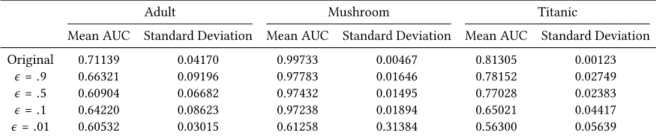
Mean AUC Standard Deviation Mean AUC Standard Deviation Mean AUC Standard Deviation Original 0.71139 0.04170 0.99733 0.00467 0.81305 0.00123

ϵ=.9 0.66321 0.09196 0.97783 0.01646 0.78152 0.02749

ϵ=.5 0.60904 0.06682 0.97432 0.01495 0.77028 0.02383

ϵ=.1 0.64220 0.08623 0.97238 0.01894 0.65021 0.04417

ϵ=.01 0.60532 0.03015 0.61258 0.31384 0.56300 0.05639 Table 6.1.:Mean Area Under the Curve of the ROC Curve on the out-of-sample data from each data

set. Recall, this is averaged over 5 runs, with the mean score and standard deviations presented.

After fitting the BRL algorithm and our DP-BRL runs with different ϵs on these three datasets, we tested the out-of-sample accuracy of the resulting rule lists. Table A.1 in the Appendix displays similar patterns for in-sample accuracy. As expected, we witness a

6.2. Experimental Results degradation in accuracy as we increase privacy (decreasingϵ), this is expected given the more privacy, the more noise we add. However, it should be noted that this is not always the case. Moving fromϵof 0.5 to 0.1 on the Adult dataset witnesses an increase in accuracy, potentially due to a lack of convergence for MCMC on this dataset given we could not run our convergence tests for this dataset. It should also be noted that especially within the more complex datasets, the UCI Adult and Mushroom datasets, accuracy is penalized only a small amount. ϵ values of 0.9 and 0.1 yield accuracy scores within 0.07 of the original algorithm. Overall, DP-BRL withϵ = 0.1 scores decently well, staying within 0.17 of the original algorithms results for all datasets, and within 0.025 for the Mushroom dataset. It’s worth pointing out that the expected patterns of degradation are followed more closely while examining in-sample accuracy (Table A.1). These results are promising in terms of the utility of DP-BRL.

Interpretability

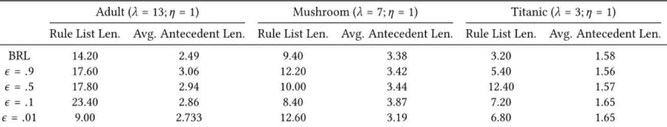
Adult (λ= 13;η= 1) Mushroom (λ= 7;η= 1) Titanic (λ= 3;η= 1) Rule List Len. Avg. Antecedent Len. Rule List Len. Avg. Antecedent Len. Rule List Len. Avg. Antecedent Len.

BRL 14.20 2.49 9.40 3.38 3.20 1.58

ϵ=.9 17.60 3.06 12.20 3.42 5.40 1.56

ϵ=.5 17.80 2.94 10.00 3.44 12.40 1.57

ϵ=.1 23.40 2.86 8.40 3.87 7.20 1.65

ϵ=.01 9.00 2.733 12.60 3.19 6.80 1.65

Table 6.2.:Mean rule list length and average antecedent lengths averaged over 5 runs, with

prefer-encesλandηfor rule list length and antecedent length respectively.

Letham et al. introduce hyperparametersλandηfor users of BRL to add their interpretability preferences into the algorithm. Given that these factors are a measure of interpretability within the original algorithm, we wish to compare our closeness to these parameters and the “interpretability” of the rule lists sampled by the original algorithm. In Table 6.2, we can see that if these are our metrics of interpretability, then the DP-BRL algorithm seems to follow the parameters far less closely than the original algorithm. In considering the simpler Titanic dataset, we can see rather arbitrary numbers for rule list length, this could have some relation to the limited set of antecedents given the size of the dataset. In contrast, rule list lengths from DP-BRL trained on the other two datasets seemed to follow the original algorithm more closely, however, they do still differ by a noticeable degree. Additionally, it is interesting to note that the average antecedent lengths for all algorithms are very close, appearing as though differential privacy had little effect in disturbing this aspect of the rule lists interpretability.

6. Experimental Results

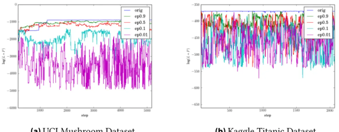
(a)UCI Mushroom Dataset (b)Kaggle Titanic Dataset

Figure 6.1.:log(score(r,N,A,λ,η,α)) for the rule list retrieved at the end of every MCMC step. Burn in not depicted.

Log Scoring, MCMC Convergence, and Scalability

Log Scoring In Figure 6.1 we plot log(score(r,D,λ,η,A)) as a function of MCMC steps. In

doing this, we can compare the log-scores of the sampled rule lists with different privacy budgets against the original BRL algorithm. Note that for the mushroom dataset with 22 categories, rule lists created with a largeϵ of 0.9 are comparable in score to a smallϵ of 0.5. What’s more is that theseϵ values also score similarly to the original algorithm, which makes us believe that utilizing a somewhat small privacy budget does not significantly harm the utility of the algorithm given a more feature-complex dataset. On a simpler dataset, such as the Titanic dataset with only 6 attributes, results may seem sporadic and low-utility, however we observe a window of around 100, which is a fairly small range (log(100)≈ 5), within which these scores land in Figure 6.1b for low values ofϵ. These observations are fortified by our findings in the previous section on accuracy analysis.

6.2. Experimental Results

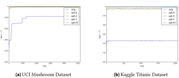
(a)UCI Mushroom Dataset (b)Kaggle Titanic Dataset

Figure 6.2.:Convergence of MCMC as a function of score over steps. Burn in included.

MCMC Convergence To determine convergence of MCMC for our different algorithms, we

run our chains for a fixed number of steps, splitting the runs into windows of 250 steps. After these runs, we check that the scores of the rule lists from the last two windows are within [−0.05n,0.05n] of each other, wherenis the number of records in the dataset. Utilizing this methodology, all five algorithms converged for our two test datasets.

Moving onto figure 6.2 we observe that our MCMC mixes well over time. We utilize each algorithms respective scoring function to gauge convergence here (for the original algorithm: u(r), and ϵ2

2∆uu(r) for DP-BRL, whereu(r) = log(score(r,D,λ,η,A))), and it should be noted

that we count the first 170 and 70 steps as burn-in for the trials on the Mushroom and Titanic datasets respectively. Additionally it can be seen in figure 6.2a that differential privacy, and subsequently smaller privacy budgets, cause MCMC to converge earlier within the same dataset. Intuitively, this is caused byϵdampening the scores we calculate for each rule list. The smallerϵ, the closer our scores are the 0 and the less variety between them, allowing our MCMC to mix faster.

Dataset: Adult Mushroom Titanic

Time Time Time

BRL 392.566 43.906 1.597

ϵ=.9 386.833 44.177 2.568 ϵ=.5 354.940 38.554 2.809 ϵ=.1 335.519 34.813 2.556 ϵ =.01 248.485 30.816 2.125

6. Experimental Results

Scalability Table 6.3 shows algorithm run times. From these results, patterns seem to arise

from both the size of the dataset, but also the complexity of it. We observe a vast increase in run time from the Titanic to Mushroom datasets, which can be attributed to the complexity of the datasets and the size disparity. Additionally if we compare the timing of the original BRL algorithm to our DP-BRL runs within the Adult and Mushroom datasets, we can see a decrease in run times as our privacy budget decreases, giving us improved scalability, seemingly at a trade off with accuracy. The time difference reaching over two minutes per run forϵ = 0.01 on the Adult dataset.

7. Conclusion

7.1. Contributions

This paper has introduced DP-BRL, a differentially private version of the Bayesian Rule List algorithm introduced by Letham et al. [17]. In doing so we analyzed the algorithm as three separate components, and performed a literature review to gain an understanding of ways to potentially privatize the differing parts. Once our methods of privatization were determined, we calculated the sensitivities (see Chapter 5) necessary and proved the privacy for each subroutine. Through experimentation on the completed algorithm, we were able to perform critical analyses of the effects of our privacy budgetϵon the interpretability, accuracy and scalability of our model. While the original Letham et al. algorithm bests our algorithm in both interpretabilty and accuracy, we believe this degradation is manageable and a necessity when promising privacy. Additionally, the improvements to run time through the addition of differential privacy may make the algorithm more attractive to some users, offsetting the setbacks to accuracy and interpretability. As for the interpretability of rule lists retrieved from DP-BRL, we hope further investigation can unpack our seemingly arbitrary results.

7.2. Future Work

For the future, we hope that a full suite of experiments can be run on DP-BRL with a differen-tially private frequent itemset mining algorithm in place. Tests for utility and interpretability would be both useful and interesting to examine after this modification. Moreover, it would be interesting to drop our privatization subroutines into the Scalable Bayesian Rule Lists algorithm by Yang et al. [26] for an even faster, more scalable interpretable machine learning algorithm with differential privacy. In addition, we would be interested in running our algorithm on a server or cluster to test accuracy and efficiency on larger, real world datasets. The effects of noise due to privacy on an algorithms accuracy can can be mitigated by database size, and so the experimental utility would be nice to see on sets of larger size. Further, given the lack of correlation between the interpretability hyperparameters and the lengths of rule lists retrieved from DP-BRL, we are interested in investigating ways to modify

7. Conclusion

DP-BRL in order to improve interpretability. In a similar vein, we believe that some usability testing would be of interest to gauge interpretability. For now, we gauge interpretability by λandη, but interviewing users of the current BRL algorithm, and potential users could be of interest to understand what truly determines interpretability, and how much our differential privatization effects these factors.

To close, our code is open sourced and publicly available on GitHub1for any future work and innovation that may come. We encourage the inspired reader to continue off our work in this paper, and to contribute to the growing fields of differential privacy and interpretable machine learning.

1_{https://git.io/DP-BRL}

A. Appendix

Theorems

Theorem 3. Sampling fromscore(r,N,A,λ,η,α)is notϵ-differentially private

Proof. For sampling fromscore(r,N,A,λ,η,α) to beϵ-differentially private, we need there to existϵsuch that exp(−ϵ) ≤ score(r,N,A,λ,η,α)

score(r,N0,A,λ,η,α) ≤ exp(ϵ). score(r,N,A,λ,η,α)

score(r,N0_,A,λ,η,α) =

Likelihood(N,r,α)∗Prior(r|A,λ,η) Likelihood(N0_{,r,α)∗Prior(r|A,λ,η)}

Since we utilize the same rule listr, and the prior does not correlate to the data, we can further simplify: Likelihood(N,r,α)∗Prior(r|A,λ,η) Likelihood(N0,r,α)∗Prior(r|A,λ,η) = Likelihood(N,r,α) Likelihood(N0,r,α) = Qm j=0 Γ(Nj,0+α0)Γ(Nj,1+α1) Γ(Nj,0+Nj,1+α0+α1) Qm j=0 Γ(N0 j,0+α0)Γ(N 0 j,1+α1) Γ(N0 j,0+Nj0,1+α0+α1) Recall any data point is captured by only one rule and one label, contributing to one count ofN_i0_,1orN_i0_,0, without loss of generality, let’s assume our missing point was captured by N0

i,0. Then, for alli 6=j, our numerator and denominator cancel out, leaving us with:

Qm j=0 Γ(Nj,0+α0)Γ(Nj,1+α1) Γ(_Nj,0+Nj,1+α0+α1) Qm j=0 Γ(N_j0_,0+α_0)Γ(N_j0_,1+α₁₎ Γ(N0 j,0+Nj0,1+α0+α1) = Γ(Ni,0+α0)Γ(Ni,1+α1) Γ(Ni,0+Ni,1+α0+α1) Γ(N_i0_,0+α_0)Γ(N_i0_,1+α₁₎ Γ(N0 i,0+Ni0,1+α0+α1) = Γ(Ni,0+α0)Γ(Ni,1+α1) Γ(Ni,0+Ni,1+α0+α1) Γ(Ni,0+α0−1)Γ(Ni,1+α1) Γ(Ni,0+Ni,1+α0+α1−1) = Γ(Ni,0+α0) Γ(Ni,0+Ni,1+α0+α1) Γ(Ni,0+α0−1) Γ(Ni,0+Ni,1+α0+α1−1) = (Ni,0+α0−1)!(Ni,0+Ni,1+α0+α1−2)! (Ni,0+α0−2)!(Ni,0+Ni,1+α0+α1−1)! = Ni,0+α0−1 Ni,0+Ni,1+α0+α1−1.

To minimize this, we wantNi,0 as small as possible, soNi,0 = 1, noteNi,0 >0 given the data

point concerned was captured byNi,0. Maximizing the denominator, we wantNi,1as large as possible, soNi,1=n−1, so _n+11 ≤ Ni,0+α0−1

Ni,0+Ni,1+α0+α1−1. Note that asn → ∞then 1

n+1 → 0 and

@ϵ such that exp(−ϵ) ≤ 0< _scorescore₍(_rr_,,_NN0,_,A,λ,η,α)

A. Appendix

Tables

Adult Mushroom Titanic

Mean AUC Standard Deviation Mean AUC Standard Deviation Mean AUC Standard Deviation Original 0.83159 0.00347 0.96521 0.00883 0.83191 0.00026

ϵ=.9 0.81652 0.00591 0.96586 0.00251 0.80088 0.02982

ϵ=.5 0.81024 0.00378 0.95815 0.00565 0.79669 0.024615

ϵ=.1 0.77889 0.01559 0.87845 0.03401 0.66865 0.06099

ϵ=.01 0.72638 0.04993 0.76669 0.08074 0.57981 0.07639 Table A.1.:Mean Area Under the Curve of the ROC Curve for all five algorithms on our three datasets

(in-sample). This is averaged over 5 runs, with the mean score and standard deviations presented.

Bibliography

[1] Learning from data. InData Mining. IEEE, 2009.

[2] M. Abadi, A. Chu, I. Goodfellow, H. B. McMahan, I. Mironov, K. Talwar, and L. Zhang. Deep learning with differential privacy. In Proceedings of the 2016 ACM SIGSAC Conference on Computer and Communications Security, CCS ’16, pages 308–318, New York, NY, USA, 2016. ACM.

[3] R. Bhaskar, S. Laxman, A. Smith, and A. Thakurta. Discovering frequent patterns in sensitive data. InProceedings of the 16th ACM SIGKDD international conference on Knowledge discovery and data mining - KDD '10. ACM Press, 2010.

[4] N. Carlini, C. Liu, J. Kos, Ú. Erlingsson, and D. X. Song. The secret sharer: Measuring unintended neural network memorization & extracting secrets. CoRR, abs/1802.08232, 2018.

[5] K. Chaudhuri, C. Monteleoni, and A. D. Sarwate. Differentially private empirical risk minimization. J. Mach. Learn. Res., 12:1069–1109, July 2011.

[6] Z. Che, S. Purushotham, R. G. Khemani, and Y. Liu. Interpretable deep models for icu outcome prediction. AMIA ... Annual Symposium proceedings. AMIA Symposium, 2016:371–380, 2016.

[7] D. Dheeru and E. Karra Taniskidou. UCI machine learning repository, 2017.

[8] J. Dressel and H. Farid. The accuracy, fairness, and limits of predicting recidivism. Science Advances, 4(1), 2018.

[9] C. Dwork. Differential privacy. In33rd International Colloquium on Automata, Lan-guages and Programming, part II (ICALP 2006), volume 4052, pages 1–12, Venice, Italy, July 2006. Springer Verlag.

[10] C. Dwork, F. McSherry, K. Nissim, and A. Smith. Calibrating noise to sensitivity in private data analysis. InProceedings of the Third Conference on Theory of Cryptography, TCC’06, pages 265–284, Berlin, Heidelberg, 2006. Springer-Verlag.

[11] C. Dwork and A. Roth. The algorithmic foundations of differential privacy.Foundations and Trends® in Theoretical Computer Science, 9(3-4), 2013.

Bibliography

[12] M. Fredrikson, S. Jha, and T. Ristenpart. Model inversion attacks that exploit confidence information and basic countermeasures. In Proceedings of the 22Nd ACM SIGSAC Conference on Computer and Communications Security, CCS ’15, pages 1322–1333, New York, NY, USA, 2015. ACM.

[13] A. Friedman and A. Schuster. Data mining with differential privacy. InProceedings of the 16th ACM SIGKDD International Conference on Knowledge Discovery and Data Mining, KDD ’10, pages 493–502, New York, NY, USA, 2010. ACM.

[14] Z. Ji, Z. C. Lipton, and C. Elkan. Differential privacy and machine learning: a survey and review. CoRR, abs/1412.7584, 2014.

[15] Kaggle. Titanic: Machine learning from disaster. https://www.kaggle.com/c/ titanic/data, 2016. [Online; accessed 3-April-2018].

[16] G. J. Katuwal and R. Chen. Machine learning model interpretability for precision medicine. 2016.

[17] B. Letham, C. Rudin, T. H. McCormick, and D. Madigan. Interpretable classifiers using rules and bayesian analysis: Building a better stroke prediction model. The Annals of Applied Statistics, 9(3):1350–1371, sep 2015.

[18] B. Li, C. Chen, H. Liu, and L. Carin. On connecting stochastic gradient mcmc and differential privacy. 12 2017.

[19] D. J. C. MacKay. Information theory, inference & learning algorithms. Cambridge University Press, New York, NY, USA, 2002.

[20] F. McSherry. Privacy integrated queries. Communications of the ACM, 53(9):89, sep 2010.

[21] A. Narayanan and V. Shmatikov. How to break anonymity of the netflix prize dataset. CoRR, abs/cs/0610105, 2006.

[22] E. Shen and T. Yu. Mining frequent graph patterns with differential privacy. In Proceedings of the 19th ACM SIGKDD international conference on Knowledge discovery and data mining - KDD '13. ACM Press, 2013.

[23] L. Sweeney. k-Anonymity: A model for protecting privacy. International Journal of Uncertainty, Fuzziness and Knowledge-Based Systems, 10(05):557–570, oct 2002.

[24] J. Vaidya, B. Shafiq, A. Basu, and Y. Hong. Differentially private naive bayes classifi-cation. InProceedings of the 2013 IEEE/WIC/ACM International Joint Conferences on Web Intelligence (WI) and Intelligent Agent Technologies (IAT) - Volume 01, WI-IAT ’13, pages 571–576, Washington, DC, USA, 2013. IEEE Computer Society.

Bibliography [25] Y.-X. Wang, S. E. Fienberg, and A. Smola. Privacy for free: Posterior sampling and

stochastic gradient monte carlo. 02 2015.

[26] H. Yang, C. Rudin, and M. I. Seltzer. Scalable bayesian rule lists. InICML, 2017. [27] S. Yıldırım. On the use of penalty mcmc for differential privacy. 04 2016.

[28] C. Zeng, J. F. Naughton, and J.-Y. Cai. On differentially private frequent itemset mining. Proc. VLDB Endow., 6(1):25–36, Nov. 2012.

[29] J. Zhang, Z. Zhang, X. Xiao, Y. Yang, and M. Winslett. Functional mechanism: Regres-sion analysis under differential privacy. PVLDB, 5:1364–1375, 2012.