Two-stage Framework for Visualization
of Clustered High Dimensional Data
Jaegul Choo∗College of Computing Georgia Institute of Technology 266 Ferst Drive, Atlanta, GA 30332, USA
Shawn Bohn†
National Visualization and Analytics Center Pacific Northwest National Laboratory 902 Battelle Blvd, Richland, WA 99354, USA
Haesun Park∗
College of Computing Georgia Institute of Technology 266 Ferst Drive, Atlanta, GA 30332, USA
ABSTRACT
In this paper, we discuss dimension reduction methods for 2D vi-sualization of high dimensional clustered data. We propose a two-stage framework for visualizing such data based on dimension re-duction methods. In the first stage, we obtain the reduced dimen-sional data by applying a supervised dimension reduction method such as linear discriminant analysis which preserves the original cluster structure in terms of its criteria. The resulting optimal re-duced dimension depends on the optimization criteria and is of-ten larger than 2. In the second stage, the dimension is further re-duced to 2 for visualization purposes by another dimension reduc-tion method such as principal component analysis. The role of the second-stage is to minimize the loss of information due to reducing the dimension all the way to 2. Using this framework, we propose several two-stage methods, and present their theoretical character-istics as well as experimental comparisons on both artificial and real-world text data sets.
Keywords: dimension reduction, linear discriminant analysis,
principal component analysis, orthogonal centroid method, 2D pro-jection, clustered data, regularization, generalized singular value decomposition
Index Terms: H.5.2 [INFORMATION INTERFACES AND
PRE-SENTATION]: User Interfaces—Theory and methods
1 INTRODUCTION
Within the visual analytics community, various types of informa-tion content are represented using high dimensional signatures. To make these signatures useful they often need to be transformed into a lower dimension (i.e., 2D or 3D) for a variety of visual represen-tations such as scatter plots. Many researchers in this community have used a wide assortment of dimension reduction techniques, e.g., self-organizing map (SOM) [12], principal component analy-sis (PCA) [11], multidimensional scaling (MDS) [2], etc. However, it is not always clear why a certain technique has been chosen over another, especially to the end user. Typically, its goal can be viewed in terms of two aspects: efficiency and accuracy. Efficiency as de-fined here is the time to compute the reduction, but accuracy may not be as simple to quantify. Many would amiably agree to quan-tify accuracy as a measure of the relationship preservation in the high dimensional space to the reduced dimensional space. Note that most techniques either directly or indirectly work on this principle. There are other properties that are important to those interpreting the semantics of the reduced space. Specifically, we note that while local neighbor preservation is important it depends upon the anal-ysis task. No single reduction technique will provide the complete view as various properties of the space are obscured or lost. We have mentioned that typically the primary objective is relationship preservation. However, there are at least two others: outlier and macro structure visualization. Outliers are conceptually easy (i.e., a variance beyond some threshold), but more difficult to quantify,
∗e-mail:{joyfull, hpark}@cc.gatech.edu
†e-mail:[email protected]
as we do not necessarily know which set of outliers are important to accentuate to the user. Certain techniques (e.g., PCA) tend to show outliers more readily, however tend to compress the reduced space at the expense of showcasing the outliers. Other techniques (e.g., SOM) maximize space usage well, but do so at the expense of masking or even hiding those outliers. Likewise, macro struc-tures of the high dimensional space may be masked or massively distorted during the reduction. Macro structures are those larger or-der groupings (e.g., clusters) that exist in the original dimensional space. We recognize they are important in dimension reduction re-search and to those in the visual analytics community. However, few of them focus on data representation especially for visualiza-tion of the clustered data [20, 13, 3].
We propose theoretical measures for these properties and effi-cient algorithms which will aid not only the researchers but ul-timately the users/analysts to better understand which balance of properties are important and for which analytic tasks.
2 MOTIVATION
The focus of this paper is the fundamental characteristics of dimen-sion reduction techniques for visualizing high dimendimen-sional data in the form of a 2D scatter plot when the data has cluster structure. The role of dimension reduction here is to give a 2-dimensional representation of data while preserving cluster structure as much as possible. To this end, supervised dimension reduction methods that incorporate cluster information such as linear discriminant analy-sis (LDA) [4] or orthogonal centroid method (OCM) [10] can be naturally considered.
However, one of the issues is that with many dimension reduc-tion methods designed to preserve the cluster structure in the data, the theoretically optimal reduced dimension, which is the smallest dimension that is acceptable with respect to the optimization crite-ria of the dimension reduction method, is usually larger than 2. For example, in LDA, the minimum reduced dimension that preserves the cluster structure quality measure defined as a trace maximiza-tion problem is one less than the number of clusters in the data in general [8, 7].
In this case, one may simply choose the two dimensions that contribute most to such a measure. However, with only two dimen-sions, such a measure may become significantly smaller than the original quantity after dimension reduction. This results in loss of information that hinders visualization in properly reflecting the true cluster relationship of the data. A similar situation may occur when using PCA for visualizing the data not having a cluster structure. Even though PCA finds the principal axes that maximally capture the variance of the data, when the resulting 2-dimensional repre-sentation of the data maintains only a small fraction of the total variance, the relationships of the data in 2 dimension are likely to be highly inconsistent with those in the original dimension.
Such loss of information is inevitable in that the dimension has to be reduced to 2. Our main motivation is to deal with such loss more carefully by separating the loss-introducing stage from the origi-nal dimension reduction methods. Based on this idea, we propose the two-stage framework of dimension reduction for visualization.
In this framework, a supervised dimension reduction method is ap-plied in the first stage so that the original dimension is reduced to the minimum dimension achievable while preserving the quality of cluster measure as defined in a dimension reduction method. The reduced dimension achieved in the first stage is often larger than 2. Thus in the second stage, we find another dimension reducing transformation that minimizes the loss introduced in further reduc-ing the dimension all the way to 2. This two-stage framework pro-vides us with a means to flexibly apply different types of dimension reduction techniques in each stage and to systematically analyze their effects, which provides understanding the effects of the over-all dimension reduction methods for visualization of clustered data. The issues then are the design of the most appropriate dimension reduction methods, the modeling of optimization criteria, and the corresponding solution methods.
In this paper, we present both theoretical and empirical answers to these issues. Specifically, we propose several two-stage methods utilizing linear dimension reduction methods such as LDA, orthog-onal centroid method (OCM), and principal component analysis (PCA), and we present their theoretical justifications by modeling the optimization criteria for which each method provides the opti-mal solution. Also, we illustrate and compare the effectiveness of the proposed methods by showing empirical visualization on syn-thetic and real-world data sets.Although nonlinear dimension re-duction methods such as MDS or other manifold learning methods such as isometric feature mapping [16] and locally linear embed-ding [14] may also be utilized for the effective 2D visualization of high dimensional data, our focus in this paper is on linear methods. The linear methods are computationally more efficient in general, and unlike most of the manifold learning methods, they also provide dimension reducing transformations that can be applied to map and visualize unseen data points in the same space where the existing data are visualized.
Our approach to successively apply two dimension reduction methods should be discerned from the previous works [18, 19, 21] in that they usually aim for improving computational effi-ciency, scalability, or applicability of a certain dimension reduction method, e.g., LDA.
The rest of this paper is organized as follows. In Section 3, LDA, OCM, and PCA are described based on a unified framework of the scatter matrices and their trace optimization problems. In Section 4, we formulate two-stage dimension reduction methods, and in Sec-tion 5, several two-stage methods for visualizaSec-tion are proposed and compared along with their criteria. Experimental comparisons are given using artificial and real-world data sets in Section 6, and con-clusion and future work are addressed in Section 7.
3 DIMENSION REDUCTION AS TRACE OPTIMIZATION
PROBLEM
In this section, we introduce the notions of scatter matrices used in defining cluster quality and optimization criteria for dimension reduction.
Suppose a dimension reducing linear transformationGT∈Rl×m
maps an m-dimensional data vector x to a vector z in an
l-dimensional space (m>l):
GT:x∈Rm×1→z=GTx∈Rl×1. (1)
Suppose also that a data matrixA= [a1a2· · ·an]∈Rm×nis given
where the columnsaj,j=1, . . . ,n,ofArepresentndata items in
anm-dimensional space, and they are partitioned intok clusters.
Without loss of generality, for simplicity of notations, we further
assume thatAis partitioned as
A= [A1 A2 · · · Ak],whereAi∈Rm×niand
k
∑
i=1ni=n.
LetNi denote the set of column indices that belong to clusteri,
andnithe size ofNi. Thei-th cluster centroidc(i)and the global
centroidcare defined, respectively, as
c(i)= 1 ni j
∑
∈N i ajandc= 1 n n∑
j=1 aj.The scatter matrix within the i-th cluster S(wi), the within-cluster
scatter matrix Sw, the between-cluster scatter matrixSb, and the
total (or mixture) scatter matrixStare defined [9, 15], respectively,
as S(wi) =
∑
j∈Ni (aj−c(i))(aj−c(i))T, Sw = k∑
i=1 S(wi)= k∑
i=1j∑
∈Ni (aj−c(i))(aj−c(i))T, (2) Sb = k∑
i=1j∈∑
Ni (c(i)−c)(c(i)−c)T= k∑
i=1 ni(c(i)−c)(c(i)−c)T = 1 n k−1∑
i=1 k∑
j=i+1 ninj(c(i)−c(j))(c(i)−c(j))T,and (3) St = n∑
j=1 (aj−c)(aj−c)T. (4)Note that the total scatter matrixStis related toSwandSbas [9]
St=Sw+Sb. (5)
WhenGT in Eq. (1) is applied to the matrixA, the scatter matrices
Sw,Sb, andStin the original dimensional space are reduced to the
l×lmatrices
GTSwG,GTSbG,andGTStG,
respectively. By computing the trace of the scatter matrices as
trace(Sw) = k
∑
i=1j∑
∈Ni (aj−c(i))T(aj−c(i)) = k∑
i=1j∑
∈Ni kaj−c(i)k22, (6) trace(Sb) = k∑
i=1j∑
∈Ni (c(i)−c)T(c(i)−c) = k∑
i=1 nikc(i)−ck22 (7) = 1 n k−1∑
i=1 k∑
j=i+1 ninjkc(i)−c(j)k22,and (8) trace(St) = n∑
j=1 (aj−c)T(aj−c) = n∑
j=1 kaj−ck22, (9) we obtain values that can be used to measure the cluster quality.Note that from Eqs. (7) and (8), trace(Sb)can be viewed as the
squared sum of the pairwise distances between cluster centroids as well as that of the distances between each centroid and the global centroid.
The cluster structure quality can be defined by analyzing how well each cluster can be discriminated from each other. High
qual-ity clusters usually have small trace(Sw)and large trace(Sb),
re-lating to the small variance within each cluster and the large dis-tances between clusters. Subsequently, dimension reduction
meth-ods may be intended to maximize trace(GTS
trace(GTS
wG)in the reduced dimensional space. This
simultane-ous optimization can be approximated to a single criterion as
Jb/w(G) =max trace((GTSwG)−1(GTSbG)), (10)
which is the criterion of LDA. In addition, one may focus on maxi-mizing the distances between clusters, which can be represented as the criterion of OCM, i.e.,
Jb(G) = max
GTG=Itrace(G
TS
bG). (11)
On the other hand, regardless of cluster dependent terms,Sw and
Sb, the trace of the total scatter matrixStcan be maximized as
Jt(G) = max
GTG=Itrace(G
T
StG), (12)
which turns out to be the criterion of PCA. In Eqs. (11) and (12),
without the constraint,GTG=I,Jb(G)andJt(G)can become
ar-bitrarily large.
In what follows, LDA, OCM, and PCA are discussed based on such maximization criteria, and their properties relevant to visual-ization are identified.
3.1 Linear Discriminant Analysis (LDA)
Conceptually, in LDA, we are looking for a dimension reducing transformation that keeps the between-cluster relationship as
re-mote as possible by maximizing trace(GTS
bG)while keeping the
within cluster relationship as compact as possible by minimizing
trace(GTS
wG). As shown in Eq. (10), the criterion of LDA can be
written as
Jb/w(G) =max trace((GTSwG)−1(GTSbG)). (13)
It can be shown that for anyG∈Rm×lwherem>l,
trace((GTSwG)−1(GTSbG))≤trace(S−w1Sb), (14)
meaning that the cluster structure quality measured by trace(S−1
w Sb)
cannot be increased after dimension reduction [4]. By setting the
derivative of Eq. (13) with respect toGto zero, which gives the
first order optimality condition, it can be shown that the solution
of LDA, where we denote it asGLDA,has the columns which are
the leading generalized eigenvectorsuof the generalized eigenvalue
problem,
Sbu=λSwu. (15)
Since the rank ofSbis at mostk−1, LDA achieves the upper bound
of trace((GTS
wG)−1(GTSbG))in Eq. (14) for anylsuch thatl≥
k−1, i.e.,
trace((GTLDASwGLDA)−1(GTLDASbGLDA))
=trace(S−w1Sb)forl≥k−1, (16)
which indicates trace(S−1
w Sb) is preserved between the original
space and the reduced dimensional space obtained byGLDA.
3.2 Orthogonal Centroid Method (OCM)
Orthogonal centroid method (OCM) [10] focuses only on
maximiz-ing trace(GTS
bG)under the constraint ofGTG=I. The criterion
of OCM is shown as
Jb(G) = max
GTG=Itrace(G
T
SbG). (17)
It is known that for anyG∈Rm×lwherem>lsuch thatGTG=
I,
trace(GTSbG)≤trace(Sb), (18)
which means the cluster structure quality measured by trace(Sb)
cannot be increased after dimension reduction. The solution of Eq.
(17) can be obtained by setting the columns ofGas the leading
eigenvectors ofSb. SinceSbhas at mostk−1 nonzero eigenvalues,
the upper bound of trace(GTS
bG)in Eq. (18) can be achieved for
anylsuch thatl≥k−1, i.e.,
trace(GTSbG) =trace(Sb)forl≥k−1. (19)
Eq. (19) indicates trace(Sb)is preserved between the original and
the reduced dimensional spaces.
An advantage of OCM is that it achieves an upper bound of
trace(GTS
bG)more efficiently by using QR decomposition,
avoid-ing the eigendecomposition. The algorithm of OCM is as
fol-lows. First the centroid matrix C is formed so that each
col-umn ofCis composed of each cluster’s centroid vector, i.e.,C=
c1 c2 · · · ck
. Then the reduced QR decomposition [5] of
Cis computed forC=QkRwhereQk∈Rm×kwithQTkQk=Iand
R∈Rk×kis upper triangular. The solution of OCM,GOCM, is found
as
GOCM=Qk.
Note that the columns ofGOCM are composed of the orthogonal
bases for the subspace spanned by the centroids, andl=kin this
case. Finally, OCM achieves
trace(GT
OCMSbGOCM) =trace(Sb),wherel=k.
By using the equivalence between Eqs. (3) and (3), one can prove that each pairwise distance between cluster centroids is also preserved in the reduced dimensional space obtained by OCM.
Another important property of OCM is that by projecting data into the subspace spanned by the centroids, the order of similarities between any particular point and centroids are preserved in terms of Euclidean norm and cosine similarity measure [10, 7]. In other
words, for any vectorq∈Rm×1and cluster centroidsc(i)andc(j),
we have
kq−c(i)k2<kq−c(j)k2⇒
kGTOCMq−GTOCMc(i)k2<kGTOCMq−GTOCMc(j)k2,and
qTc(i) kqk2kc(i)k2 < q Tc(j) kqk2kc(j)k2 ⇒ GT OCMq T GT OCMc(i) kGTOCMqk2kGTOCMc(i)k2 < G T OCMq T GT OCMc(j) kGTOCMqk2kGTOCMc(j)k2 .
3.3 Principal Component Analysis (PCA)
PCA is a well-known dimension reduction method that captures the maximal variance in the data. The criterion of PCA can be written as
Jt(G) = max
GTG=Itrace(G
TS
tG). (20)
For anyG∈Rm×lwherem>lsuch thatGTG=I, we have
trace(GTStG)≤trace(St), (21)
which means trace(St)cannot be increased after dimension
reduc-tion. The solution of Eq. (20), where we denote it asGPCA, can
be obtained by setting the columns ofGas the leading
eigenvec-tors ofSt. Since the rank ofStis at most min(m,n), PCA achieves
the upper bound of trace(GTS
tG)in Eq. (21) for anylsuch that
l≥min(m,n), i.e.,
Table 1: Comparison of dimension reduction methods. It is assumedSbandStare full rank.
LDA OCM PCA
Optimization Criterion (x∈Rm×1G→Ty∈Rl×1) Jb/w(G) = max trace((GTS wG)−1(GTSbG)) Jb(G) = max GTG=Itrace(G TS bG) Jt(G) = max GTG=Itrace(G TS tG)
Algorithm generalized eigendecomposition QR decomposition symmetric eigendecomposition
Smallest dimension achieving
the criterion upper bound k−1 k min(m,n)
In many applications of PCA, however, l is usually chosen as a
fixed value less than the ranke ofSt for the purpose of dimension
reduction or noise reduction. This noisy subspace corresponds to
the smallest eigenvectors ofSt, and they are removed by PCA for
better representation of the data.
AlthoughSt is related to Sb andSw as in Eq. (5), St as it is
does not contain any information on cluster labels. That is, unlike LDA and OCM, PCA ignores the cluster structure represented by
Sband/orSw, which is why PCA is considered as an unsupervised
dimension reduction method.
Usually, PCA assumes that the global centroid is zero by sub-tracting the empirical mean of the data from each data vector.
The centered data can be represented as A−ceT, where eis
n-dimensional vector whose components are all 1’s.
PCA has a unique property that, given a fixedl, it produces the
best reduced dimensional representation that minimizes the
differ-ence between the centered matrixA−ceT and its projection to the
reduced dimensional spaceGGT(A−ceT)whereGhas
orthonor-mal columns, i.e.,
GPCA=arg min
G,GTG=IlkGG
T(A−ceT)−(A−ceT)k,
where the matrix normk · kis either a Frobenius norm or a
Eu-clidean norm.
The three discussed methods are summarized in Table 1.
4 FORMULATION OFTWO-STAGEFRAMEWORK FOR
VISU-ALIZATION
Suppose we want to find a dimension reducing linear
transforma-tionVT∈R2×mthat maps anm-dimensional data vectorxto a
vec-torzin a 2-dimensional space (m≫2):
VT:x∈Rm×1→z=VTx∈R2×1. (22)
Further assume that it is composed of two stages of dimension re-ductions as follows. In the first stage, a dimension reducing linear
transformationGT∈Rl×mmaps anm-dimensional data vectorxto
a vectoryin thel-dimensional space (l≪m):
GT:x∈Rm×1→y=GTx∈Rl×1, (23)
wherelis fixed as its minimum optimal dimension by the first-stage
criterion. Whenl≤2, we have no further dimension reduction to
do after the first step. However, an optimallin many methods and
for many data sets is larger than 2, and so we assume thatl>2.
In the second stage, another dimension reducing linear
transfor-mationHT∈R2×lmaps anl-dimensional data vectoryto a vector
zin the 2-dimensional space(l>2):
HT:y∈Rl×1→z=HTy∈R2×1. (24)
Such consecutive dimension reductions performed byGT
fol-lowed byHT can be combined, resulting in a single dimension
re-ducing transformationVTas
VT=HTGT. (25)
In the next section, discussion will be focused on various ways
for choosing the first stage dimension reducing transformationG
and the second stage dimension transformationHwith a purpose
to construct combined dimension reducing transformationVT =
HTGT for 2-dimensional visualization according to various
opti-mization criteria.
5 TWO-STAGEMETHODS FOR2D VISUALIZATION
All the proposed two-stage methods start from one of the super-vised dimension reduction methods such as LDA or OCM that are
designed for clustered data. In the first stage (byGT ∈Rl×m in
Eq. (23)), the dimension is reduced by LDA or OCM to the small-est dimension that satisfies Eq. (16) or (19), respectively. There-fore in the first stage, the cluster structure quality measured either
by trace(S−1
w Sb)or trace(Sb)is preserved. Then we perform the
second-stage dimension reduction (byHT∈R2×lin Eq. (24)) that
minimizes the loss of information either by applying the same
cri-terion used in the first stage or by usingJtin Eq. (20), i.e., that of
PCA. As seen in Section 3.3, Eq. (20) gives the best approxima-tion of the first-stage results that minimize the difference in terms of Frobenius/Euclidean norm.
In what follows, we describe each of the two-stage methods in
detail, and derive their equivalent single-stage methods (byVT ∈
R2×min Eq. (22)) in case they exist.
5.1 Rank-2 LDA
In this method, LDA is applied in the first stage, and trace(S−1
w Sb)
is preserved in thel-dimensional space wherel=k−1. In the
second stage, the same criterionJb/w(H)is used to reduce the
l-dimensional first-stage results to 2-l-dimensional data.
The criterion of the second-stage dimension reducing matrixH
can be formulated as Hb/w= max H∈Rl×2trace((H T(GT LDASwGLDA)H)−1 (HT(GTLDASbGLDA)H)). (26)
Assuming the columns ofGLDA, which are generalized
eigenvec-tors of Eq. (15), are in decreasing order of their corresponding
gen-eralized eigenvalues, i.e.,GLDA=
u1 u2 · · · uk−1
where
λ1≥λ2≥ · · · ≥λk−1, the solution of Eq. (26) is
Hb/w=
e1 e2
,
where e1 and e2 are the first and the second standard unit
vectors, i.e., e1 =
1 0 · · · 0 T
∈ Rl×1 and e2 =
0 1 0 · · · 0 T
∈Rl×1. This solution is equivalent to
choosing two dimensions with the most leading generalized eigen-values from the first stage result, and the resulting two-stage method can be represented as a single-stage dimension reduction method by
V∈Rm×2which directly maximizeJb/w, i.e.,
Vb/w = arg max V∈Rm×2Jb/w(V) = arg max V∈Rm×2trace((V TS wV)−1(VTSbV)). (27)
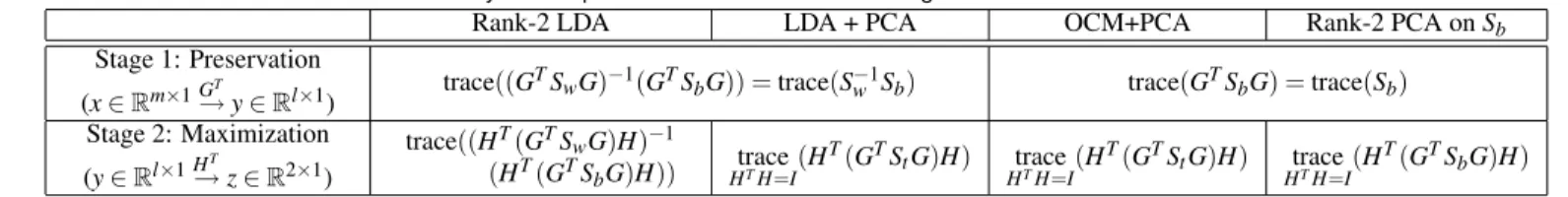
Table 2: Summary of the optimization criteria of the two-stage dimension reduction methods.
Rank-2 LDA LDA + PCA OCM+PCA Rank-2 PCA onSb
Stage 1: Preservation
(x∈Rm×1→GTy∈Rl×1) trace((G
TS
wG)−1(GTSbG)) =trace(Sw−1Sb) trace(GTSbG) =trace(Sb)
Stage 2: Maximization (y∈Rl×1H→Tz∈R2×1) trace((HT(GTS wG)H)−1 (HT(GTS bG)H)) trace HTH=I(H T(GTS tG)H) trace HTH=I(H T(GTS tG)H) trace HTH=I(H T(GTS bG)H)
The solution of Eq. (27) becomes
Vb/w=GLDAHb/w=
u1 u2 ,
where u1and u2 are the leading generalized eigenvectors of Eq.
(15). This solution is also known as reduced-rank linear discrim-inant analysis [6].
5.2 LDA followed by PCA
In this method, LDA is applied in the first stage, and trace(S−1
w Sb)is
preserved in thel-dimensional space wherel=k−1. In the second
stage, PCA is applied in order to obtain the best approximation of
thel-dimensional first-stage results in terms of Frobenius/Euclidean
norm.
The second-stage dimension reducing matrixHis obtained by
solving
Ht=arg max
H∈Rl×2,HTH=Itrace(H
T(GT
LDAStGLDA)H), (28)
where the solution is the two leading eigenvectors of the total scatter
matrix of the first-stage result,GTLDAStGLDA.
From Eq. (5), we have
GTLDAStGLDA=GLDAT (Sb+Sw)GLDA. (29)
Since LDA conceptually maximizes trace(GTS
bG)and minimizes
trace(GTS
wG), the result is expected to satisfy
trace(GTLDASbGLDA)≫trace(GTLDASwGLDA)),
which means thatGTLDAStGLDAis dominated byGTLDASbGLDA, i.e.,
GTLDA(Sb+Sw)GLDA≃GTLDASbGLDA.
In this case, the principal axes that PCA gives in the second stage better reflect those of the between-cluster matrix of the first-stage
result,GTLDASbGLDA, and they may in turn discriminate the clusters
clearly in the 2-dimensional space. In this sense, LDA followed by PCA achieves a clear cluster structure as well as a good approxima-tion of the first-stage result.
5.3 OCM followed by PCA
In this method, OCM is applied in the first stage, and trace(Sb)is
preserved in thel-dimensional space wherel=k. In the second
stage, PCA is applied in order to obtain the best approximation of
thel-dimensional first-stage results in terms of Frobenius/Euclidean
norm.
As in Section 5.2, the second-stage dimension reducing matrix
His obtained by solving
Ht=arg max
H∈Rl×2,HTH=Itrace(H
T(GT
OCMStGOCM)H), (30)
where the solution is the two leading eigenvectors of the total scatter
matrix of the first-stage result,GTOCMStGOCM.
From Eq. (5), we have
GTOCMStGOCM=GOCMT (Sb+Sw)GOCM. (31)
Unlike LDA, OCM does not minimize trace(GTS
wG)as shown in
Eq. (17). Therefore the following may not be the case:
trace(GTOCMSbGOCM)≫trace(GTOCMSwGOCM),
which means that GTOCMSbGOCM does not necessarily dominate
GT
OCMStGOCM. Then the two principal axes ofGTOCMStGOCM
ob-tained by PCA in the second stage tend to fail to reflect those of
GTOCMSbGOCM, which may rather scatter the data points within
each cluster, eventually preventing the visualization results from showing a clear cluster structure.
5.4 Rank-2 PCA onSb
In this method, OCM is applied in the first stage, and trace(Sb)is
preserved in thel-dimensional space wherel=k. In the second
stage, the same criterionJb(H)is used to reduce thel-dimensional
first-stage results to 2-dimensional data.
The second-stage dimension reducing matrixHis obtained by
solving
Hb=arg max
H∈Rl×2,HTH=Itrace(H
T(GT
OCMSbGOCM)H), (32)
where the solution is the two leading eigenvectors of the
between-scatter matrix of the first-stage result,GTOCMSbGOCM. The columns
ofGOCM form the subspace spanned by centroids, and this
sub-space includes the range sub-space ofSb. Accordingly, one can easily
show that the eigenvectoruYi ∈Rl×1ofGTOCMSbGOCMis related to
eigenvectorsui∈Rm×1ofSbas
uYi =GTOCMui
with their corresponding eigenvalues matched as well, i.e.,λY
i =λi.
Hence, the solution of Eq. (32) can be written as
Hb= uY1 uY2 =GTOCM u1 u2 . (33)
Using Eq. (33) and the relationship shown in Eq. (25), the
single-stage dimension reducing transformationVbcan be built as
VbT = HbTGTOCM= uT1 uT2 GOCMGTOCM = uT 1 uT2 (34) = arg max V∈Rm×2Jb(V) = arg max V∈Rm×2trace(V T SbV). (35)
Eq. (34) holds since the eigenvectors ofSb,u1andu2, are in the
range space ofGOCM. The criterion of Eq. (35) has been used in
one of the successful visual analytic systems, IN-SPIRE, for 2D representation of document data [17].
The discussed two-stage methods are summarized in Table 2.
6 EXPERIMENTS
In this section, we present visualization results using the proposed methods for several data sets, especially focusing on undersam-pled text data visualization where the data item is represented in
m-dimensional space and the number of the data itemsnis less
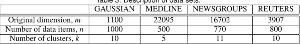
Table 3: Description of data sets.
GAUSSIAN MEDLINE NEWSGROUPS REUTERS
Original dimension,m 1100 22095 16702 3907
Number of data items,n 1000 500 770 800
Number of clusters,k 10 5 11 10
6.1 Regularization on LDA for undersampled data
In undersampled cases, the LDA criterion shown in Eq. (13)
can-not be applied directly becauseSw is singular. In order to
over-come this singularity problem, Howland et al. proposed a univer-sal algorithmic framework of LDA using the generalized singular value decomposition (LDA/GSVD) [8, 7]. Specifically, for the case
when m≫n≫k, which is usual for most undersampled
prob-lems, LDA/GSVD gives the solution forGsuch thatGTSwG=0
while maintaining the maximum value of trace(GTS
bG). This
so-lution makes sense since LDA criterion is formulated to minimize
trace(GTS
wG). However, it means that all of the data points
be-longing to a specific cluster are represented as a single point in the reduced dimensional space, which lessens the generalization abil-ity for classification as well as for visualizing the individual data relationship within each cluster.
On the contrary, the fact that LDA makesGTSwG=0 can be
viewed as an advantage for visualization purposes since LDA has
the capability to fully minimize trace(GTS
wG). By means of
regu-larization onSwone can control trace(GTSwG), which determines
the scatter of the data points within each cluster. In regularized LDA
which was originally proposed to avoid the singularity ofSwin
clas-sification context,Swis replaced by a nonsingular matrixSw+γI
whereIis an identity matrix, andγis a control parameter. In
gen-eral, asγis increased, the within-cluster distance, trace(GTS
wG),
also becomes larger with data points being more scattered around
their corresponding centroids. Asγis decreased, the within-cluster
distance becomes smaller, and the data points gather closer around
their centroids. Such manipulation ofγcan be exploited in a
vi-sualization context because one can choose an appropriate value of
γso that the second-stage method such as PCA, which maximizes
trace(GTS
tG) =trace(GTSbG+GTSwG), does not focus too much
on trace(GTS
wG). The results that follow are based on such choices
ofγ.
6.2 Data Sets
The data sets tested are composed of one artificially-generated Gaussian-mixture dataset (GAUSSIAN) and three real-world text data sets (MEDLINE, NEWSGROUPS, and REUTERS) that are clustered based on their topics. All the text documents are encoded as term-document matrices where each dimension corresponds to a particular word, and the value of a certain dimension represents the frequency of the corresponding word shown in the document. Each data set is set to have an equal number of data per cluster, and have a mean of zero which is attained by subtracting the global mean. (See Section 6.3.)
The descriptions of data sets, which are also summarized in Ta-ble 3, are as follows.
The GAUSSIAN data set is a randomly generated Gaussian mix-ture with 10 clusters. Each cluster is made up of 100 data vectors, which add up to 1000 in total, and the dimension is set to 1100, which is slightly more than the number of the data items. In its vi-sualization shown in Fig. (1), the clusters are labeled using letters as
• ’a’, ’b’,. . ., and ’j’.
The MEDLINE data set is a document corpus related to medical
science from the National Institutes of Health1. The original
di-mension is 22095, and the number of clusters is 5, where each
clus-1http://www.cc.gatech.edu/˜hpark/data.html
ter has 100 documents. The cluster labels that correspond to the document topics are shown as
• heart attack (’h’), colon cancer (’c’), diabetes (’d’), oral cancer
(’o’), and tooth decay (’t’),
where the letters in parentheses are used in the visualization shown in Fig. (2).
The NEWSGROUPS data set [1] is a collection of newsgroup documents, and originally composed of 20 topics. However, we have chosen 11 topics for visualization, and each cluster is set to have 70 documents. The original dimension is 16702, and the clus-ter labels are shown as
• comp.sys.ibm.pc.hardware (’p’), comp.sys.mac.hardware (’a’),
misc.forsale (’f’), rec.sport.baseball (’b), sci crypt (’y’),
sci.electronics (’e’), sci.med (’d’), soc.religion.christian (’c’),
talk.politics.guns (’g’), talk.politics.misc (’p’), and talk.religion.misc (’r’),
where the letters in parentheses are used in the visualization shown in Fig. (3).
The REUTERS data set [1] is the document collection that ap-peared in the Reuters newswire in 1987, and originally composed of hundreds of topics. Among them, 10 topics related to economic subjects are chosen for visualization, and each cluster has 80 doc-uments. The original dimension is 3907, and the cluster labels are shown as
• earn (’e’), acquisitions (’a’), money-fx (’m’), grain (’g’), crude (’r’),
trade (’t’), interest (’i’), ship (’s’), wheat (’w’), and corn (’c’), where the letters in parentheses are used in the visualization shown in Fig. (4).
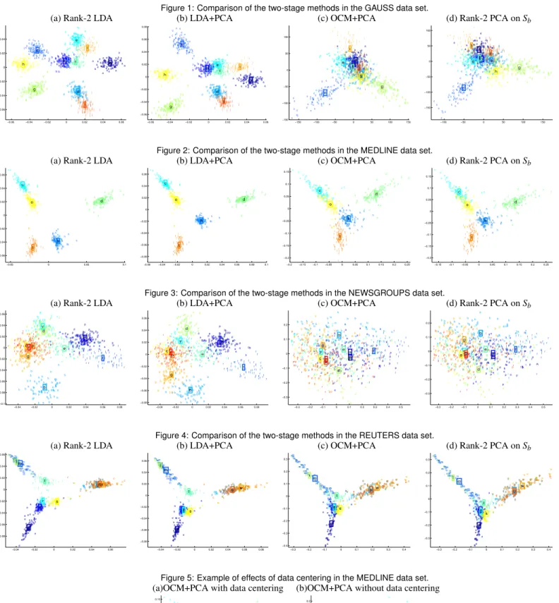
6.3 Effects of Data Centering
Fig. 5 is the example of applying OCM+PCA to the MEDLINE data set with and without data centering. Once the MEDLINE data set is encoded as a term-document matrix, every component has a non-negative value, which results in the global centroid that is sig-nificantly far from the origin. Then performing PCA without data centering might give the first principal axis as the one reflecting the global centroid rather than that discriminating clusters. If we con-sider projecting the data onto each of the horizontal and the vertical axes in Fig. 5, the former, which corresponds to the first princi-pal axis, does not help in showing the cluster structure clearly, and only the vertical axis, which corresponds to the second principal axis from PCA, discriminates clusters. We have found that such undesirable behavior is common in many cases without data center-ing, which is why we assume that data is centered throughout this paper. Accordingly, all the results shown in Figs 1-4 are obtained after data centering.
6.4 Comparison of Visualization Results
The results of four two-stage methods for the tested data sets are
shown in Figs.1-42.
In all cases, LDA-based methods show cluster structures more clearly than OCM-based methods. This proves the effectiveness of LDA that considers both within- and between-cluster measures while OCM only takes into account the latter. Due to this differ-ence, OCM generally produces a widely-scattered data representa-tion within each cluster. As a result, in the NEWSGROUPS dataset, such a wide within-cluster variance significantly deteriorates the
2Those figures can be arbitrarily magnified without losing the resolution
cluster structure visualization even if OCM still attempts to max-imize the between-cluster distance.
In the MEDLINE and the REUTERS data sets, all of the four
methods produce relatively similar results. However, we have
controlled the within-cluster variance in LDA-based methods
us-ing the regularization termγI. In addition, the fact that rank-2
LDA and LDA+PCA produce almost identical results indicates that
GT
LDAStGLDAis dominated byGTLDASbGLDAafter LDA is applied in
the first stage as we expected.
Rank-2 LDA represents each cluster most compactly by mini-mizing the within-cluster radii both in the first and the second stage. However, it may reduce the between-cluster distances as well
be-causeJb/wmaximizes the conceptual ratio of two scatter measures.
As can be seen in the two LDA-based methods applied to the NEW-GROUPS data set, while rank-2 LDA minimizes the within-cluster radii, it also places the centroids closer to each other as compared to those in LDA+PCA. Due to this effect, which one is preferable between rank-2 LDA and LDA+PCA depends on the data set to be visualized.
Overall, OCM+PCA and Rank-2 PCA onSb show similar
re-sults. It meansGTSbG≃GTStGin that the difference between two
methods lies in whether PCA is applied toGTSbGorGTStGin the
second stage. Since performing PCA onGTSbGis
computation-ally more efficient than PCA onGTStG, Rank-2 PCA onSbcan be
a good alternative to OCM+PCA in case efficient computation is important.
Finally, these visualization results reveal the interesting clus-ter relationships underlying in the data. In Fig. (2), the clusclus-ters for colon cancer (’c’) and oral cancer (’o’) are shown close to each other. In Fig. (3), the clusters of soc.religion.christian (’c’) and talk.religion.misc (’r’), those of comp.sys.ibm.pc.hardware (’p’) and comp.sys.mac.hardware (’a’), and those of sci.crypt (’y’) and sci.med (’d’) are closely located respectively in LDA-based
methods. In addition, the two clusters, misc.forsale (’f’) and
rec.sport.baseball (’b’), are shown to be the most distinctive, which makes sense because those topics are quite irrelevant to the others. In Fig. (4), the clusters of grain (’g’), wheat (’w’), and corn (’c’) as well as those of money-fx (’m’) and interest (’i’) are visualized very close.
7 CONCLUSION ANDFUTUREWORK
According to our results, LDA-based methods are shown to be superior to OCM-based methods since both within- and between-cluster relationships are taken into account in LDA. Especially, combined with PCA in the second stage, LDA+PCA achieves a clear discrimination between clusters as well as the best approx-imation of the results of LDA when the distance between data is measured in terms of Frobenius/Euclidean norm.
However, many classes except for few of them that are clearly unrelated tend to be overlapped especially when dealing with large numbers of data points and clusters. This is inherently due to the nature of the second-stage dimension reduction in which only the two axes are chosen so that the classes which contribute most to the second stage criteria can be well-discriminated. Such behavior can exaggerate the distances between particular clusters, and more elaboration towards new criteria that fits in visualization is required. In the MEDLINE and the REUTERS datasets, visualization results seem to have a tail-shape along specific directions. We often found this phenomenon to occur in many other data sets. It is still unclear as to what causes this and how it affects the visualization, e.g. char-acteristics of information loss in the second stage. Finally, in order to determine how much loss of information is introduced by each method, more rigorous analysis based on various quantitative mea-sures such as pairwise between-cluster distance and within-cluster radii should be conducted.
ACKNOWLEDGEMENTS
The work of these authors was supported in part by the National Science Foundation grants CCF-0732318 and CCF-0808863. Any opinions, findings and conclusions or recommendations expressed in this material are those of the authors and do not necessarily re-flect the views of the National Science Foundation.
REFERENCES
[1] A. Asuncion and D. Newman. UCI machine learning repository. Uni-versity of California, Irvine, School of Information and Computer Sci-ences, 2007.
[2] T. F. Cox and M. A. A. Cox.Multidimensional Scaling. Chapman &
Hall, London, 1994.
[3] I. S. Dhillon, D. S. Modha, and W. S. Spangler. Class visualization of
high-dimensional data with applications. Computational Statistics &
Data Analysis, 41(1):59 – 90, 2002.
[4] K. Fukunaga. Introduction to Statistical Pattern Recognition, second
edition. Academic Press, Boston, 1990.
[5] G. H. Golub and C. F. van Loan.Matrix Computations, third edition.
Johns Hopkins University Press, Baltimore, 1996.
[6] T. Hastie, R. Tibshirani, and J. Friedman.The Elements of Statistical
Learning: Data Mining, Inference, and Prediction. Springer, 2001. [7] P. Howland, M. Jeon, and H. Park. Structure preserving dimension
re-duction for clustered text data based on the generalized singular value
decomposition. SIAM Journal on Matrix Analysis and Applications,
25(1):165–179, 2003.
[8] P. Howland and H. Park. Generalizing discriminant analysis using
the generalized singular value decomposition. Pattern Analysis and
Machine Intelligence, IEEE Transactions on, 26(8):995–1006, Aug. 2004.
[9] A. Jain and R. Dubes. Algorithms for clustering data. Prentice-Hall,
Inc. Upper Saddle River, NJ, USA, 1988.
[10] M. Jeon, H. Park, and J. B. Rosen. Dimensional reduction based on centroids and least squares for efficient processing of text data. In
Proceedings of the First SIAM International Workshop on Text Mining. Chiago, IL, 2001.
[11] I. Jolliffe.Principal component analysis. Springer, 2002.
[12] T. Kohonen.Self-organizing maps. Springer, 2001.
[13] Y. Koren and L. Carmel. Visualization of labeled data using linear
transformations. InInformation Visualization, 2003. INFOVIS 2003.
IEEE Symposium on, pages 23–30, Oct. 2003.
[14] S. T. Roweis and L. K. Saul. Nonlinear Dimensionality Reduction by
Locally Linear Embedding.Science, 290(5500):2323–2326, 2000.
[15] D. L. Swets and J. J. Weng. Using discriminant eigenfeatures for
image retrieval.IEEE Transactions on Pattern Analysis and Machine
Intelligence, 18(8):831–836, 1996.
[16] J. B. Tenenbaum, V. d. Silva, and J. C. Langford. A Global
Geo-metric Framework for Nonlinear Dimensionality Reduction.Science,
290(5500):2319–2323, 2000.
[17] J. A. Wise. The ecological approach to text visualization. Journal
of the American Society for Information Science, 50(13):1224–1233, 1999.
[18] J. Ye and Q. Li. A two-stage linear discriminant analysis via
qr-decomposition. Pattern Analysis and Machine Intelligence, IEEE
Transactions on, 27(6):929–941, June 2005.
[19] H. Yu and J. Yang. A direct LDA algorithm for high-dimensional data
with application to face recognition. Pattern Recognition, 34:2067–
2070, 2001.
[20] X. Zhang, C. Myers, and S. Kung. Cross-weighted fisher discriminant
analysis for visualization of dna microarray data. InAcoustics, Speech,
and Signal Processing, 2004. Proceedings. (ICASSP’04). IEEE Inter-national Conference on, volume 5, pages V–589–92 vol.5, May 2004. [21] W. Zhao, R. Chellappa, and A. Krishnaswamy. Discriminant analysis
of principal components for face recognition. Automatic Face and