Delineation of Road Networks from Remote Sensor Data with Deep Learning

(1)

Delineation of Road Networks from Remote Sensor Data

with Deep Learning

Pinjing Xu

A Thesis in

The Department of

Computer Science and Software Engineering

Presented in Partial Fulfillment of the Requirements for the Degree of Master of Computer Science at

Concordia University Montréal, Québec, Canada

November 2019

(2)

C

ONCORDIA

U

NIVERSITY School of Graduate Studies

This is to certify that the thesis prepared

By: Pinjing Xu

Entitled: Delineation of Road Networks from Remote Sensor Data with Deep Learning

and submitted in partial fulfillment of the requirements for the degree of Master of Computer Science

complies with the regulations of this University and meets the accepted standards with respect to originality and quality.

Signed by the Final Examining Committee:

Chair Dr. N. Shiri Examiner Dr. T.D. Bui Examiner Dr. A. Krzyzak Supervisor Dr. C. Poullis Approved by

Dr. Lata Narayanan, Chair

Department of Computer Science and Software Engineering

November 2019

Dr. Amir Asif, Dean

(3)

Abstract

Delineation of Road Networks from Remote Sensor Data with Deep Learning

Pinjing Xu

In this thesis we address the problem of semantic segmentation in geospatial data. We investigate different deep neural network architectures and present a complete pipeline for extracting road net-work vector data from satellite RGB orthophotos of urban areas.

Firstly, we present a network based on the SegNeXt architecture for the semantic segmentation of the roads. A novel loss function is introduced for training the network. The results show that the pro-posed network produces on average better results than other state-of-the-art semantic segmentation techniques. Secondly, we propose a fast post-processing technique for vectorizing the rasterized segmentation result, removing erroneous lines, and refining the road network. The result is a set of vectors representing the road network. We have extensively tested the proposed pipeline and provide quantitative comparisons with other state-of-the-art based on a number of known metrics. This work has been published and presented at the14thInternational Symposium on Visual Com-puting, 2019.

Finally, we present an altogether different approach to road extraction. We reformulate the task of extracting vectorized road networks as a deep reinforcement learning problem with partially observable state-space and present our preliminary results and future work.

(4)

Acknowledgments

I would like to express my sincere gratitude to my supervisor Dr. Charalambos Poullis who never stop encouraging, inspiring and guiding me in the past two years. Without his persistent help, my master study would not have been as substantial as today.

This research is based upon work supported by the Natural Sciences and Engineering Research Council of Canada Grants DG-N01670 (Discovery Grant) and DND-N01885 (Collaborative Re-search and Development with the Department of National Defence Grant).

(5)

List of Figures

Figure 2.1 AlexNet architecture . . . 4

Figure 2.2 VGG16 architecture . . . 5

Figure 2.3 ResNet block . . . 5

Figure 2.4 Image Segmentation Example: Horses Image . . . 6

Figure 2.5 FCN architecture . . . 7

Figure 2.6 Deconvolutional network architecture . . . 8

Figure 2.7 U-Net Architecture . . . 9

Figure 3.1 System overview . . . 15

Figure 3.2 SegNeXt-variant architecture . . . 16

Figure 3.3 Small patch size vs. large patch size. . . 18

Figure 3.4 MSE Loss Function . . . 19

Figure 3.5 Generate ground truth image for ISPRS Potsdam dataset . . . 21

Figure 3.6 ISPRS Potsdam dataset imagery is out-of-date . . . 22

Figure 3.7 OSM data mistakes . . . 23

Figure 3.8 Refinement process . . . 24

Figure 3.9 Segmentation and post-processing results . . . 25

Figure 3.10 Cities exhibiting different characteristics . . . 28

Figure 3.11 Result comparison . . . 29

Figure 4.1 CartPole-v1 Environment . . . 33

Figure 4.2 Reinforcement learning system . . . 34

(8)

Figure 4.4 RL Mesh Envirinment . . . 37 Figure 4.5 Preliminary Results of Deep Reinforcement Learning Approaches . . . 40

(9)

List of Tables

Table 3.1 Numeric results comparison . . . 26 Table 3.2 Improvement of post-processing . . . 27

(10)

Chapter 1

Introduction

The automatic extraction of road networks from remote sensor imagery has long been a challenge not just to the GIS but also the computer vision communities. The vast variations in the road functions [e.g. rural, urban, highways, etc], colors [e.g. dirt road, asphalt] , shapes [e.g. wind-ing mountain roads, straight highways], and sizes, make it an extremely challengwind-ing task. Recent attempts using deep learning techniques have shown promising results [56], [47], the majority of which reformulate the problem as a pixel classification problem and employ semantic segmentation techniques. Although this is useful in some cases, the majority of the applications employing road network data, e.g autonomous driving, GIS, etc, require that the network is in vector form; and in fact, it is this vectorization or linearization of the road network pixels that is perhaps one of the most challenging tasks.

In this thesis we present a novel approach for extracting road networks in vector form. A deep convolutional neural network based on the SegNeXt architecture is trained to classify road pixels in satellite images of urban areas. This architecture offers a reduced number of parameters and high localization accuracy therefore eliminating the need for the typical refinement of the segmentation results using MRF-based techniques. Furthermore, a novel loss function is proposed which provides better results than the typical loss functions used. The segmentation result is then vectorized and refined using a fast post-processing technique. During the post-processing, linear road segments are extracted using an iterative patch-based Hough transform technique which tracks the segments from one patch to the other. Next, a refinement process ensures that the nearby linear road segments

(11)

are connected together to form a larger road network, and conflicting/overlapping parallel segments and other small segments are removed. The final result of the proposed technique is a road network in vector form which can be readily used in any GIS-based application.

In addition, we present preliminary results of a proposed technique based on deep reinforcement learning. In order to overcome the aforementioned limitations with generating vectorized data, we reformulate the problem as one of training an agent with reinforcement learning to move along road centerlines; and in doing so directly generating a road network graph. We present the learning environment, and details on the training of the agent using two typical deep reinforcement learn-ing techniques namely, deep Q-learnlearn-ing (DQN) and Asynchronous Advantage Actor-Critic (A3C). Finally, we discuss the feasibility of utilizing deep reinforcement learning for road extraction. In summary, in this thesis:

• we present a complete and efficient pipeline for solving the problem of road extraction from satellite imagery, in which a SegNeXt-like deep neural network is used, with a novel loss function.

• we propose a new post-processing technique for the vectorization of road data from semantic segmentation results.

• we reformulate road extraction as a deep reinforcement learning problem with partially-observable state-space.

1.1 Thesis Organization

The rest of the thesis is organized as follows: Chapter 2 provides a brief overview of the state-of-the-art related to our work, including procedural and deep-learning approaches in computer vision. In Chapter 3 we present a semantic segmentation-based technique for road network extraction with a novel post-processing method. Chapter 4 describes a novel technique for road extraction using deep reinforcement learning and presents preliminary results. Finally, in Chapter 5 we present the conclusion and future work.

(12)

Chapter 2

Literature Review

Below we provide a brief overview of the state-of-the-art most relevant to our work.

2.1 Deep Learning in Computer Vision

2.1.1 Image Classification

Image classification has been a core task in computer vision in the recent decades. Before deep neural networks were introduced into the field, the classic procedure of image classification was first extracting features from the image, building feature descriptors, and then using machine learning classifiers to classify the images. One such well known technique was Bag-of-Words, which was first published by Salton & McGill in 1983 [54]. The main idea of Bag-of-Words model is to treat the frequency of occurrence of each word in a text as a feature for training a classifier. Though originally designed to represent text information in natural language processing, the concept of Bag-of-words was later brought into the field of computer vision. When classifying images, local features are first extracted using feature detectors, such as the Scale-Invariant Feature Transform (SIFT [36]) interest point detector, and then a descriptor is formed for a small region around each feature point. SIFT descriptor is commonly used in this process. A codebook is then generated from all possible features, and each image can be represented as a histogram of the codebook and used for the training of a classifier. Using the Bag-of-Features technique, Sivic & Zisserman [62] developed an approach called Video Google, that can achieve immediate run-time object retrieval

(13)

throughout a movie database.

Figure 2.1: AlexNet architecture [30]. Due to the hardware limitations, the authors trained the network on two GPUs, and combined the outputs in the last dense layer to generate labels for different categories.

ImageNet database [17] is a large visual database that contains more than 14 million hand-annotated images in more than20,000categories. In 2012, Krizhevshy designed the first modern deep neural network (AlexNet [30]) for the purpose of image classification, and won the ImageNet Large Scale Visual Recognition Challenge (ILSVRC [53]). Figure 2.1 shows the architecture of AlexNet. It contains five convolutional layers followed by three fully connected layers, max-pooling layers and ReLU activation function are also applied. The trained network achieved an error rate of16.4%, where as the winner in 2011 had an error rate around 26%. This was a breakthrough for both deep learning and image classification area. In the next few years, all the winners of the ILSVRC challenge were using deep learning models and the classification error rate fell to only a few percent.

Following the step of AlexNet, the VGG16 [59] architecture was proposed two years later. By the time, the most common way of getting better results from convolutional neural networks is to make the network deeper. So the VGG16 network, as shown in Figure 2.2 is designed to have sixteen convolutional layers, with multiple max-pooling layers and three fully connected layers at the end.3×3kernel filters is used, instead of the kernel size of11×11used in AlexNet. The smaller kernel size helps to decrease the number of parameters to train. VGG16 architecture reached7.3% top-5 error rate on the 2014 ILSVRC challenge.

(14)

Figure 2.2: VGG16 architecture [13]. Gray blocks are convolutional layers, red blocks are max-pooling layers, blue blocks are fully connected layers, and green block is the output layer to deter-mine a label from the1000categories.

6.7%. It is composed of22 layers using inception modules for a total of over 50 convolutional layers. Although it has a similar performance as the VGG16 network, the size of the model is much smaller than VGG16 due to the three fully connected layers used in VGG16 which take a large amount of space to store.

Figure 2.3: ResNet block proposed in [24].

The authors in [24] showed that by increasing the depth of the network the error rate also in-creases. Residual networks were then introduced to alleviate this problem. Residual learning cre-ates connections between the output of multiple convolutional layers and their original input with an identity mapping. Consequently, features from the training images can be learned faster in deeper layers. The so called ResNet architecture, which won the 2015 ILSVRC challenge with an error rate of3.57%, contains154convolutional layers with3×3filters using residual learning by block of two layers. An example of ResNet block structure is shown in Figure 2.3

(15)

(a) Origin (b) LA (c) SMC

(d) Human (e) EAMS (f) NC

Figure 2.4: Image segmentation example on horse image [29]. 2.4a: Original Image, 2.4b: Local Variation Algorithm [21], 2.4c: Spectral Min Cut [19], 2.4d: Human Labeled [37] [38], 2.4e: Edge Augmented Mean Shift [12] [11], 2.4f: Normalized Cut [57] [15]

2.1.2 Semantic Segmentation

Image segmentation is a pixel-wise classification problem, where every pixel in an image has to be assigned a label. Generally in a segmentation result, pixels with the same label should share similar visual characteristics, such as color, intensity, texture, etc. Thus, image segmentation is not only of interest to artificial intelligent and computer vision communities, but also widely used in image compression, image editing, and many other image processing techniques. The procedural methods of segmenting images are more or less depending on thresholds. Figure 2.4 shows an example of the performance of some classic image segmentation algorithms on a test image.

Unlike ordinary segmentation that partitions the image with only low-level cues, such as color and intensity, semantic segmentation tries to partition the image by considering the semantic mean-ing of pixels and classifies them into one of the pre-determined classes. This means semantic seg-mentation takes one more step further than image classification i.e. in addition to finding the object category similar to image classification, it also indicates the position of the object in a given image, by assigning different labels to object pixels and background pixels, or between different classes of objects; this is in contrast to image classification where only one label is required for the image as a whole. For this reason, semantic segmentation is generally considered as a harder problem than

(16)

Figure 2.5: FCN architecture [35].

image classification and ordinary segmentation.

In the past few years, following the highly active development of image classification, deep learning has also proved to be a very efficient tool for solving semantic segmentation problems. By modifying the existing deep neural networks used in image classification tasks, fully convolutional networks (FCN) [35] were purposed. The result of semantic segmentation, is an image of equal size as the input image. Figure 2.5 shows the architecture of FCN network. The authors in [35] replaced the fully connected layers used in AlexNet and VGG16 with convolutional layers to allow the network to have an arbitrary input size and corresponding output size. Then a skip connection architecture was defined that combines semantic information from the deep layer with appearance information from the shallow layer. An up-sampling at the end of the network is necessary to re-cover the reduced size caused by convolution operations. This is commonly called "deconvolution" because it generates a larger size for output than the input of this layer. The authors in [35] showed that in a FCN trained end-to-end pixels-to-pixels on semantic segmentation exceeds all procedural methods without having additional post-processing steps.

Since then, a lot of work has been done to improve the performance of FCN [8, 34, 40, 64]. In contrast to FCN, which replaces the fully connected layers in VGG16 network architecture, the authors in [47] designed a new deconvolutional network. In their work, as shown in Figure 2.6,13

(17)

Figure 2.6: Deconvolutional network architecture [47]

convolutional layers were adopted from a generic VGG16 network, and a deconvolution network consisting of a corresponding number of deconvolution and unpooling layers was used as the second part of the complete architecture. This network achieved72.5%accuracy, measured with the mean Intersection-over-Union(mIoU) metric, in the 2012 PASCAL VOC segmentation challenge [20], where the original FCN network achieved62.2%mIoU score.

Building upon the FCN architecture, U-Net [51] was proposed to solve biomedical image seg-mentation problems. Similar to the deconvolution network designed in [47], U-Net also has a series of convolutional layers and pooling layers, followed by symmetric deconvolutional layers and up-sampling layers. Feature maps from the convolutional part are integrated with the output from deconvolutional layers which helps with improving the overall precision. The architecture can be seen in Figure 2.7. Moreover, a key challenge for the development of deep learning techniques in the field of biomedical image segmentation is the relatively smaller size of the available datasets. Thousands of training images are usually beyond reach in biomedical tasks, while AlexNet in 2012 ILSVRC was trained with1million images. To solve this problem, U-Net also utilized extensive data augmentation techniques, which allowed the network to learn invariance to all kinds of defor-mations. As a result, the authors were able to train the network on a dataset that contains only30 images without overfitting.

2.2 Deep Reinforcement Learning

The first well-known method that combines reinforcement learning and deep learning is Deep Q-Learning [44]. In this work, a system that consists of a network called Deep Q-Network (DQN)

(18)

Figure 2.7: U-Net Architecture [51].

trained with a variant of Q-learning learns to play most of the Atari 2600 video games with a human-like performance. Based on this system, a lot of improvements and variants have been proposed such as the work in [23, 45, 55, 58, 67] to name a few.

Since then, most deep reinforcement learning algorithms are tested with the Atari 2600 games which have a relatively simple game environment e.g. Pong, Breakout, Space Invaders, Seaquest and Beam Rider. These games have a fixed background scene, instant reward, and only a small number of possible actions for the agent. A more complex game environment was considered in [61] called Montezuma’s Revenge. The game has sporadic and delayed reward. The agent must jump down, climb up, get the key, and open the door, and kill the monster in order to win the reward. This leads to problems in training the agent and in fact the authors report that all current techniques (circa 2017) of using deep reinforcement learning failed primarily because theε-greedy strategy fails to explore the game in a consistent and efficient manner. A similar conclusion was also mentioned in the original DQN paper in [44].

In [32], the authors designed a method that applies double Deep Q-Networks (DDQN [23]) for dynamic path planning of an unknown indoor environment. Their results shows that after training, the agent is able to reach the local target position successfully in an unknown dynamic environment.

(19)

In the work of [50], the authors created a Memory-based Deep Reinforcement Learning algorithm for robots that can explore unknown environments like indoor mazes.

Following a different approach which employs real ground-based geospatial data, the authors in [41] created a city scale interactive navigation environment called StreetLearn that uses an end-to-end reinforcement learning approach. StreetLearn takes images and underlying connectivity in-formation from Google Street View as input and can traverse and navigate from start to goal within a city. This is the first work that successfully utilizes an RL method on large-scale outdoor navigation based on real-world images instead of indoor environments or simulated outdoor environments.

2.3 Road Extraction

2.3.1 Procedural Approaches

Research aimed at extracting roads from remote sensing data automatically has been going on for more than three decades. For many years, though important progress has been made, the majority of the road extraction techniques relied solely on procedural approaches. An overview can be found in [66]. Similar to the most common techniques, authors in [2] designed an automatic algorithm to extract roads from aerial images using dynamic programming and Kalman filters. By modeling the urban and road context in different scales, authors in [26] described a new speed function con-structed using multi-spectral characteristics and road geometry. In [27], a knowledge-based system was built that could find the dominant directions of the road footprint, then initialize and track a road segment without user interaction. However it suffers from over-extraction due to the design of multi-directional road tracker. [68] determine road likelihood with superpixels and then create road networks using the shortest path algorithm and Conditional Random Field (CRF). Of the most recent, is the work in [33] where the authors propose a technique for extracting urban roads from satellite images by using orientation histograms and morphological profile features to guide a binary partition tree, thus achieving a higher accuracy.

As it is evident, all these methods mentioned above strongly rely on low-level image features, make a lot of assumptions, and require prior knowledge for the road extracting process to work. Due to the different illumination effects, appearances, and the complex environments in urban areas, such

(20)

as shadows and occlusions of buildings, trees, vehicles, etc images captured by cameras carried on airplanes or satellites can be highly variable and different. Thus, it is extremely difficult for these procedural methods to generalize on arbitrary remote sensing image datasets.

2.3.2 Deep Learning Approaches

Although generalization is a hard problem for procedural methods, it is a perfect task for modern deep learning techniques. Perhaps one of the first works on training deep neural networks for extracting large-scale road networks from satellite images is the work presented in [43]. The authors present an approach for automatically detecting roads in aerial imagery using a neural network. In this work, synthetic road/non-road labels generated from readily available vector road maps were used as ground truth labels. Firstly, principal component analysis (PCA) was applied to the RGB aerial images as pre-processing. This step was able to reduce the dimensions of the input data by two thirds and make it possible to use a large context (i.e. larger-sized patches containing a large number of urban features) for training the neural network using limited memory. By using a larger context, it is easier to better differentiate between what is a road vs a non-road pixel. Then a neural network was initialized using an unsupervised pre-training procedure proposed in [25], which has been proved better to use than initializing neural network weights randomly [25, 31]. While training the network, random angle rotations are applied to each image patch before feeding it into the network, so that the network is trained to generalize and not favor roads in any particular orientation. Lastly, as a post-processing step, a neural network was trained to refine the predictions given by the former network. This post-processing approach showed a significant improvement on the results by removing the disconnected blotches and filling in the gaps in the prediction images.

Recently, following the success of FCN, U-Net and residual block in the field of semantic segmentation, more studies in road extraction are following the semantic segmentation approach [10, 60]. Linknet architecture was proposed in [7], which takes benefit of combining U-Net archi-tecture and residual blocks from ResNet archiarchi-tecture, and using pre-trained weights from ResNet18 network as its encoder. Although ResNet18 was a light network at the time, it outperforms many other deep networks on benchmark datasets [5, 14] and the training speed is fast. On top of Linknet, D-LinkNet [74] added to the architecture dilated convolutional layers to increase the receptive fields

(21)

of feature points without decreasing the resolution of the feature maps. Also the encoder in D-LinkNet is upgraded to ResNet34 with pre-trained weights on ImageNet dataset. The network surpassed U-Net and Linknet34 and achieved64.12%IoU score during the DeepGlobe Road Ex-traction Challenge [16].

The authors in [6] propose a fully convolutional network based on the U-Net family architecture with pre-trained ResNet34 as the encoder. They optimize a loss function which combines the binary cross entropy and the intersection over union. During the test phase they report that data augmen-tation, such as randomly scaling the image by a factor between0.6−1.4and rotating the image by 30degrees, helps improve the prediction results even further.

In [73] the authors present a network which combines the ResNet and U-Net architectures to address the road network extraction. Their network employs skip connections within the residual units and between the encoding and decoding paths of the network to facilitate propagation of information, and also reduce the number of the generic U-Net’s parameters by75%.

The purpose of extracting road networks from aerial or satellite images is for using in real applications, such as autonomous driving, city planning and GIS system, where vectorized road data is required. However, the above mentioned methods are addressing road segmentation, which feeds RGB images into a deep neural network, labels the pixels as road/non-road and outputs an image that is a rasterized result. As a matter of fact, it is the vectorization or linearization of the road network pixels that is perhaps one of the most challenging tasks in road networks extraction.

The authors in [39] propose an approach named as DeepRoadMapper that estimates road topol-ogy from aerial images. Firstly, they utilize an encoder-decoder (convolution-deconvolution) net-work that consists of several ResNet blocks with a total of55convolutional layers in the encoder and3fully convolutional layers in the decoder. Skip connections are also used between convolu-tional layers in the decoder and corresponding layers in the encoder. This deep network generates an initial segmentation for roads. Then road centerlines are extracted by applying a thinning al-gorithm [72]. Treating every pixel on the centerlines as a node, a graph of the road network is generated, which is later refined and simplified using Ramer–Douglas–Peucker algorithm [18, 49]. In the latter half of the proposed pipeline, a heuristic algorithm is designed to make a hypothesis on

(22)

possible connections for gaps and missing parts in the graph. A second network built with an in-ception network [63] is then trained to classify and determine whether a hypothesized connection in the graph is correct or not. The DeepRoadMapper is a complete workflow, that takes RGB imagery as input and generates a fine-tuned road graph as their output. Their result fits the requirements of real applications, but issues still exist.

As of early 2019, the best performing road network extraction technique is RoadTracer pre-sented in [3]. Instead of using deep neural networks for semantic segmentation, the authors follow a new paradigm in which a CNN is used as a decision function for tracing the road network in the image. A searching algorithm is designed that maintains a graph and a stack of vertices in the graph. Given a known road pixel in the RGB image, a small patch around this pixel is cropped and fed into a convolutional neural network. The CNN contains17convolutional layers, with batch normalization [28] and ReLU [46] activation applied after each layer. The network has two output components: an action to decide between "GO" and "STOP", and a vector of 64elements repre-senting64orientations around the current road pixel indicating the specific orientation for the next step if the action component shows "GO". Every time the CNN decides to move i.e. "GO", a new vertex will be added to the vertex stack according to the orientation component, meanwhile this new vertex and an edge will be added into the graph. By doing so, it is possible to trace along the road in the satellite imagery. Once the CNN outputs "STOP" as the action component, the vertex stack will pop the top vertex and the tracer will jump back to the last visited vertex (top vertex in the stack) to check if there is any other options to choose (i.e. at a road junction). This approach is doing an excellent job on extracting vectorized road data with no post-processing required, but it has the pre-condition that the starting point lies on a road otherwise the tracing fails. Problems also arise in cases where tracing the road network runs out of points to process e.g. commonly occurring at bridges. In this case, the result will be partial and disjoint from the entire road network and it becomes hard to recover the missing parts.

(23)

Chapter 3

Deep Residual Neural Networks and

Iterative Hough Transform for Road

Extraction

In this chapter, we present a complete pipeline for road extraction. A SegNeXt-like network ar-chitecture trained with a novel loss function provides a semantic segmentation of roads. A novel post-processing technique then converts the segmented roads into vector form. We show that the post-processing technique produces better output when compared to other commonly used meth-ods in state-of-the-art road extraction techniques. The final result is a set of vectors representing the road network. We extensively test our network and present an analysis of the results on two benchmark datasets. This work has been published in the 14th International Symposium on Visual Computing [70].

3.1 Technical Overview

The input to our system is an RGB image which is fed forward into a deep autoencoder network (SegNeXt) with aggregated residual transformations. The network outputs a semantic segmentation of the image in the form of a grayscale image in which each pixel is classified into aroad or non-roadclasses. The classification image is then divided into patches which are further refined. During

(24)

Figure 3.1: System overview. The input RGB image is processed using SegNeXt and results in a grayscale classification image of road and non-road pixels. The classification image is then divided into patches which are further processed. The refinement process involves an iterative application of patch-based Hough transforms which results in a set of extracted lines. Erroneously extracted lines resulting from misclassification are removed, and nearby lines are either connected (if not parallel) or suppressed (if parallel). The result is a set of vectors representing the road network in the input image shown in yellow overlaid on the input image.

the refinement process, an iterative patch-based Hough transform is applied. Extracted lines are tracked from one patch to the other. Spurious lines resulting from misclassification are removed, and nearby lines are either connected (if non-parallel) or suppressed (if parallel). The result is a set of vectors representing the road network in the input image. Figure 3.1 summarizes the system overview.

3.2 Network Architecture

Although plenty of remarkable works has been done in the recent years to improve the performance of deep neural networks in the semantic segmentation task, the segmentation output of most network architectures is still coarse, due to the loss of information while applying pooling or down-sampling to the feature maps [1]. Thus, a post-processing technique, such as conditional random field to smooth and refine the segmentation result is often required. The skip connection used in U-Net is one of the solutions to this problem, where the feature maps are passed to the decoding layers from corresponding layers in the encoder, concatenated with the input to the decoder layers before apply-ing deconvolution. The SegNet architecture, proposed in [1], tries to solve the problem in another way. It stores the pooling indices while applying max-pooling, then directly passes the pooling indices to the corresponding decoder layers. During up-sampling for deconvolution, feature maps

(25)

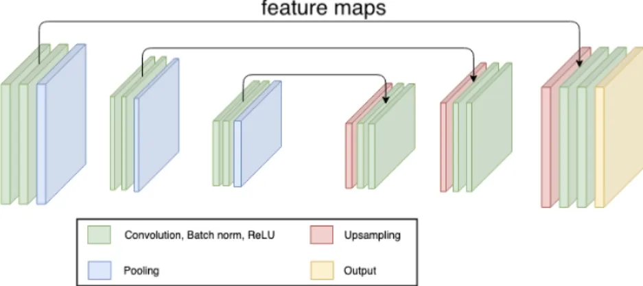
Figure 3.2: SegNeXt-variant architecture

are expanded according to the pooling indices, and the information lost during pooling operation is restored. As a result, the SegNet model is more efficient when compared to the U-Net where the entire feature maps in float precision are stored in memory.

In order to learn more detailed features from input images, most of the state-of-the-art deep neural networks try to build the network deeper and wider, as well as introducing various hyper-parameters within the architecture, e.g. atrous convolutions. However, the deeper a network, the more difficult it is for deeper layers to retain information about the input during training due to vanishing/exploding gradients. A solution to this was the ResNet block [24] which pushes the learning process at the deep layers, by having direct connections to shallower layers. In contrast to the ResNet blocks that help the network go deeper, the authors in [69] introduce the concept of "cardinality", which represents the size of the set of transformations. They demonstrated that by having a larger cardinality the networks can be built shallower and thus easier to train.

In our work, the network architecture resembles that of a SegNeXt network [22], which is a combination of a SegNet-like architecture and ResNeXt blocks [69] as shown in Figure 3.2. It consists of three deep convolutional encoders and a corresponding number of decoders with feed-forward links to pass the feature maps from the encoder layers to the decoder layers and merge it with the input of decoder layers; in contrast to the SegNet where only pooling indices are restored for up-sampling since the information lost from the pooling operation can not be fully recovered with pooling indices. The cardinality-enabled residual-based building blocks proposed in [69] are also used in our network. In each residual block the input data is split into multiple groups onto

(26)

which different kernels are applied. A dilation of 2 is applied during convolution to introduce more spatial context. Batch normalization [28] and the ReLU activation function [46] are applied at each convolutional layers. The feed-forward links from the encoders to the decoders help to retain high frequency information and improve the boundary delineation resulting in a smoother segmentation result therefore eliminating the need for any subsequent post-processing with conditional random fields (CRF), etc. In [69] these cardinality-enabled residual-based blocks used in shallow networks were shown to surpass in terms of performance other deeper CNNs. Thus, using these blocks the network can be shallower resulting in a smaller number of trainable network parameters therefore making the training process more cost-effective. In addition, the last layer that performs softmax operation in the original SegNeXt architecture, which is used for multi-class classification task, is replaced by a convolutional output layer that gives grayscale results in which the value of each pixel indicates the likelihood of it to be a road/non-road pixel.

3.3 Experiments

3.3.1 Dataset

We trained our network on two different datasets: (a) satellite imagery of Potsdam from 2D Se-mantic Labeling Contest [52] held by the International Society for Photogrammetry and Remote Sensing (ISPRS), and (b) Google Map Imagery data of40 different cities around the world. For both datasets, ground truth images are generated with road centerlines extracted from the Open-StreetMap [48] data.

Potsdam Imagery from ISPRS Benchmark Dataset

The ISPRS benchmark dataset for Potsdam contains 38RGB image tiles in total, with a pixel resolution of6K×6Kand ground sampling resolution of5cm. Of all these tiles, only24images are geo-referenced (GPS information included in the image file) and available for training neural networks. We spilt them into two sets,18images are used for training the network, and6images are for testing. The city of Potsdam shows a typical European city with relatively larger building blocks, narrower streets and dense settlement structure compared with modern cities in North America.

(27)

Google Maps Imagery

Google Maps Imagery data is very easy to use with; configurations such as location, zoom level and image resolution can be defined by the user. To make our work more comparable to the current state-of-the-art, we train and test our network following a similar approach as in [3]. 300satellite images acquired from Google Maps with resolution of4096×4096and ground sampling density of60_pixelcm (zoom level18) are used. These images are randomly selected in the24km2surrounding area of the GPS locations of40major cities.

3.3.2 Training

In order to maximize the training dataset we decided not to use a validation set during training but rather calculate the loss based after each epoch on three randomly selected patches from the training set. The training took48 hours on a single NVIDIA GTX 1080Ti with an adaptive learning rate. We have used Keras API (with Tensorflow as backend engine) for the development of the network and the code is available as open source athttps://theictlab.org/lp/2019Re_X/.

Input. It is necessary to make an appropriate choice for the patch size of the network input. If the patch is too large, it could not fit into the network due to the limited memory in GPU, and if a patch is too small it will have less coverage and therefore context which in turn will cause ambiguity when learning the features in the image as reported in [43] (see Figure 3.3). In each epoch during our training process, the input to the network is a batch of32 image patches of size200×200to make sure that the patch width is wider than the general road width in the imagery. Patches are cropped and selected from the images in the entire training set using random sampling in order to ensure appropriate coverage.

(a) (b)

Figure 3.3: An example of using small patch size vs. larger patch size given in [43]. These two images are showing the same roof top region, but with different patch size. On 3.3a, there is no way to determine the content inside the patch. On 3.3b, with a larger patch size, more context is visible to us, and helps to understand the semantic meaning of this region.

(28)

Data augmentation. We apply a series of different data augmentation operations on the input patches. A histogram equalization is first applied to all patches in order to reduce possible high con-trast resulting from deep black shadows. Next, a number of transformations is performed consisting of random rotations in the range of[0,π₂], scaling up/down by up to70%, and random flipping on the vertical/horizontal axis.

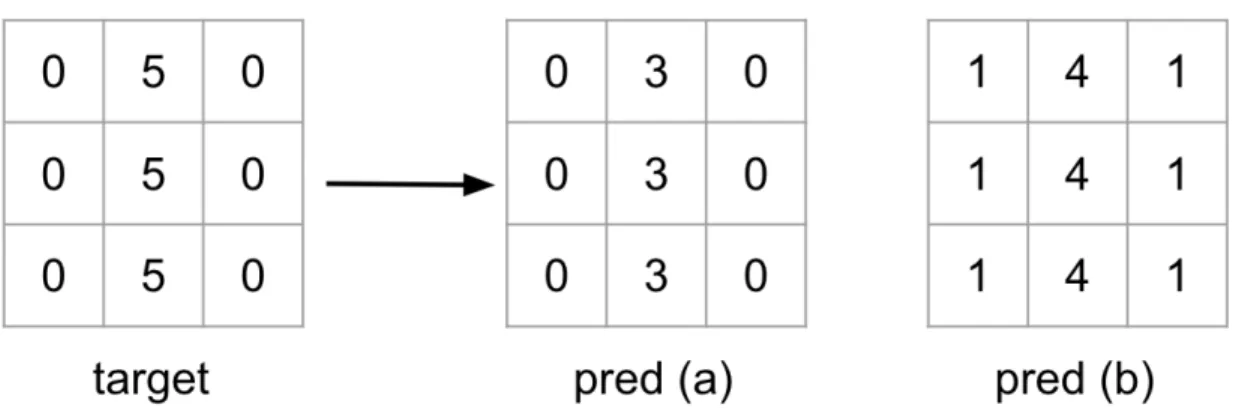
Loss function. Perhaps the most widely used loss functions when dealing with a classification problem are the (a) Mean square error(MSE), and (b) Intersection over Union(IoU). However, due to the characteristics of MSE (takes the sum of a patch but ignores the positional relationships, shown in Figure 3.4), it tends to result in a lot of noise in the segmentation output, and often yields bad performance. On the other hand, the use of an IoU loss function results in many gaps in the results as it was also recently reported in [3]. To address the aforementioned limitations, we propose a new loss function which comprises of both MSE and the inverse of IoU, and combines them as follows,

L=M SE× union

intersection (1)

Intuitively, the MSE is good at indicating whether a pixel is road or non-road, and the inverse of the IoU helps to reduce the noise.

Figure 3.4: An example of two different predictions to the same patch. MSE of prediction (a) is

12

9, MSE of prediction (b) is 9

9. Prediction (b) has a smaller loss in terms of number, but prediction

(a) is prefered in segmentation result because the edge in prediction (a) is sharper than in prediction (b), which makes it easier to choose a proper threshold value.

(29)

Training on Potsdam Imagery from ISPRS Benchmark Dataset

We had some issues while training our network on the ISPRS Potsdam dataset. The ground sampling resolution on this dataset (5cm) is too high. The range of 30cm to 60cm of ground sampling resolution is the commonly used in most of the related works. With the ground sampling resolution of5cmwe can hardly set a proper patch size for training the network. Furthermore, we tried to not only extract road centerlines from the satellite images but also the type and orientation of each extracted road. Thus, some pre-processing steps needed to be done before the actual training.

Firstly for the RGB imagery, we down-sampled all the image tiles to the pixel resolution of 600×600(was6K ×6K), so the ground sampling resolution is reduced to50cm and lies in the commonly used range. Then, while generating the ground truth images we designed an encoding that is able to include road type and orientation information into the pixel values. The encoding uses a three channel matrix, which can be visualized by an image, to store the information. The three-channel image is then compressed into a single channel image to reduce the dimensionality of the problem. The details are as follows (also see Figure 3.5):

• Extract data. Road centerlines and road type data are extracted from OpenStreetMap [48] database. Road orientations are calculated from the OSM road vector data. According to the extracted data, there are totally 11 road types appearing in the ISPRS Potsdam dataset: motorway, trunk, primary, secondary, tertiary, residential, track, pedestrian, side walk, foot way and unclassified road.

• Encode data.Encode the road information for all images with the following rules:

– Red channel:1if the pixel is road pixel, otherwise 0;

– Green channel:road orientation in the range[0,π₂], with11.25degrees increments at a time, which results in16different orientations in total;

– Blue channel:a number representing road type, if applicable, ranging in[1,11].

(30)

(a) (b)

(c) (d)

Figure 3.5: Generate ground truth image for ISPRS Potsdam dataset. 3.5a shows the RGB image tile. 3.5b shows align encoded 3-channel data with RGB imagery. 3.5c shows encoded 3-channel data without background. 3.5d shows compressed single channel data as a grayscale image.

sure each label can be mapped into an unique value by using the formula:

P ixelIntensity=R×(G×11 +B) (2)

During our experiment, we found that the training process can not reach a performance which will produce useful results. Although road pixels in the image can be labeled out by the network, the prediction is not good enough, as labels for road pixels can not be distinguished from each other. For pixels lying on the same road where the type and orientation should be identical, different labels

(31)

(a) (b) (c)

(d) (e) (f)

Figure 3.6: ISPRS Potsdam dataset imagery is out-of-date. 3.6a and 3.6d are the latest imagery download from Google Earth, 3.6b and 3.6e are the imagery in the ISPRS Potsdam dataset, 3.6c and 3.6f shows the ground truth data extracted from OpenStreetMap of the corresponding region.

were shown and there is no way to recover the correct label for the single complete road. We then tried to discard the encoding and change the labels in ground truth images into a binary format, using255vs0with respect to road vs non-road. At the same time, we widened the width of road centerlines in the ground truth images to10pixels instead of the single pixel width shown in Figure 3.5. The goal was to make the feature in the ground truth images clearer so that it won’t easily lose information during convolutional and pooling operations.

We examined both the training result and the ISPRS dataset and came up with the following conclusions:

• The ISPRS Potsdam dataset was captured at a past time and therefore did not match the latest OSM data well enough (see Figure 3.6);

• OSM data contains mistakes in the labels, and since ISPRS Potsdam has only18images in the training set, there is a large percentage of wrong examples in the training set. This makes it hard to learn correct features and also hard to evaluate. An example is shown in Figure 3.7.

(32)

Figure 3.7: Example shows OSM data mistakes. Yellow lines are road data extracted from Open-StreetMap database. It is clear to see that in the region of the red circle, the entire road is misaligned with the actual one.

For the above mentioned reasons, we concluded that the ISPRS Potsdam dataset is not appro-priate for this purpose.

Training on Google Maps Imagery

To make our work more comparable to the state-of-the-art approaches, we train and test our network following a similar approach as in [3], as well as the similar settings for dataset. Training and validation is performed using images of 25 of these cities, and testing is performed on the images of the remaining15cities. Thus, there are no images of the same city between the training and testing sets. The ground truth images are rendered with road center line data extracted from the OpenStreetMap [48], and the width of road lines is set to10pixels.

3.3.3 Inference

During inference, we run the network on the image with a sliding window, of size 200×200 and a step size of100. Instead of thresholding the semantic segmentation result similar to many

(33)

Figure 3.8: Refinement process. Three cases are considered. A: no overlap between two windows, move the two nearby end points to the average location to connect these two line segments; B: 50% overlapping between windows, in addition to merging nearby end points of line segments, the merging of nearby points-to-lines is also needed; C: extract a curve by merging nearby lines. Smaller windows size and larger overlapping area will yield smoother result.

other semantic segmentation techniques, we remove the noise and extract roads by applying Hough transform to extract line segments in each window based on the network predictions. Since we have overlaps between the sliding windows, extracted line segments may not agree in different windows. Thus, further refinement is needed to improve the result and get a clean road network.

3.3.4 Post-processing Refinement

Figure 3.8 shows all possible cases handled by our refinement process and what the resulting line segments will be. For a simple case, if there’s no overlap between two windows (patches), the extracted Hough lines will be like case A with no crossing over or overlap on one another. In this case, we merge all nearby line end points by moving them to their average location. Next, we consider the case of overlapping patches similar to case B in the Figure 3.8. If the extracted Hough lines on two patches do not match with each other, intersection or misalignment will occur. To address the misalignment issue, we perform the following steps:

(34)

2. For each line end point, search around itself for nearby lines, if there is a lineACpassing by this end point, merge this end point into the line in the following steps:

• break the lineAC;

• find the middle pointBbetween the end point and the line; • move the end point toB;

• connect the two end pointsAandCwith pointB, forming two new linesABandBC

This procedure is repeated on all line end points in the image and as a result all misaligned lines are removed. An advantage of this procedure is that although Hough transform cannot extract curved roads from the network prediction, by extracting short line segments a curved road can be approximated as a set of piece-wise linear segments connected to each other. By merging nearby points-to-points (e.g. case A) and points-to-lines (e.g. case B), we can reconstruct a curved road or a circle with Hough lines (e.g. case C).

Searching for road segments iteratively through the entire image space can be a time consuming process. Since we are using a sliding window technique during testing only neighbours of the current patch are within the search range for merging nearby points and connecting line segments. In most cases, only one or two line segments will be found on road patches. Thus, this searching and merging progress is very fast. Figure 3.9 shows an example of the network segmentation and result after post-processing.

(a) (b) (c)

Figure 3.9: An example of the network segmentation and result after post-processing. 3.9a is the RGB image, 3.9b is the segmentation output from our network, 3.9c is the final result after applying our proposed post-processing technique.

(35)

3.3.5 Evaluation

As of writing this manuscript the state-of-the-art in the area is considered to be the work presented in [3]. The authors have shown that they outperform all previously top performers in road extraction. Hence, we use the customjunction metric proposed by [3] and the well-known Intersection over Union (IoU) metric to evaluate our work and compare our results. The junction metric involves measuring the precision and recall based on the detected junctions in the inferred map. Furthermore, we report on additional metrics typically used in road extraction such as completeness, correctness, precision, recall, and F1 score.

Ours [3] RT [39] DRM

City F1 IoU Junction F1 IoU Junction F1 IoU Junction

Amsterdam 0.28 0.16 0.16 0.01 0.01 0.01 0.22 0.13 0.04 Boston 0.71 0.55 0.58 0.67 0.51 0.74 0.77 0.62 0.66 Chicago 0.58 0.41 0.41 0.69 0.52 0.77 0.68 0.51 0.51 Denver 0.71 0.56 0.57 0.69 0.53 0.73 0.46 0.30 0.35 Kansas City 0.82 0.69 0.70 0.76 0.61 0.82 0.85 0.74 0.76 Los Angeles 0.68 0.51 0.51 0.73 0.57 0.79 0.73 0.58 0.61 Montreal 0.73 0.57 0.55 0.78 0.63 0.80 0.69 0.53 0.56 New York 0.51 0.34 0.35 0.73 0.57 0.84 0.42 0.26 0.29 Paris 0.59 0.42 0.26 0.67 0.51 0.71 0.41 0.26 0.31 Pittsburgh 0.71 0.55 0.57 0.41 0.26 0.48 0.69 0.58 0.57 Salt Lake City 0.75 0.60 0.65 0.73 0.58 0.79 0.58 0.41 0.47 San Diego 0.72 0.56 0.62 0.66 0.49 0.77 0.79 0.65 0.72 Tokyo 0.38 0.24 0.11 0.56 0.39 0.60 0.42 0.27 0.34 Toronto 0.69 0.53 0.48 0.76 0.61 0.74 0.79 0.65 0.69 Vancouver 0.41 0.26 0.25 0.65 0.49 0.70 0.45 0.29 0.29

Average 0.63 0.47 0.45 0.63 0.49 0.69 0.60 0.45 0.48

Table 3.1: F1 Score, IoU and Junction metrics on 15 test cities. [3] RT: RoadTracer, [39] DRM: DeepRoadMapper (implementation provided in [3])

Table 3.1 shows the comparison between the proposed approach and the two state-of-the-art RoadTracer [3] and DeepRoadMapper [39]. The F1 Score and IoU metrics shown are for the 15 test cities. As it can be seen, our method outperforms the DeepRoadMapper on the overall test set in both F1 score and IoU metrics. Our technique also surpasses the RoadTracer in accuracy on at least half of the cities. We attribute this to the fact that our approach initially results in a very high number of classified roads which the refinement process then prunes down, leading to a lower error

(36)

rate than the other techniques.

In terms of the junction metric, the results show that both semantic segmentation methods (ours and DeepRoadMapper) have the same level of performance in detecting the junctions, whereas the RoadTracer performs better because it seldom misclassifies road pixels around junctions.

Ours (w/ PP) Ours (w/o PP) DRM [39] DRM (w/ PP)

City F1 IoU F1 IoU F1 IoU F1 IoU

Amsterdam 0.28 0.16 0.26 0.15 0.22 0.13 0.21 0.12 Boston 0.71 0.55 0.62 0.45 0.77 0.62 0.80 0.67 Chicago 0.58 0.41 0.44 0.29 0.68 0.51 0.74 0.58 Denver 0.71 0.56 0.64 0.47 0.46 0.30 0.55 0.38 Kansas City 0.82 0.69 0.78 0.64 0.85 0.74 0.88 0.79 Los Angeles 0.68 0.51 0.57 0.39 0.73 0.58 0.77 0.63 Montreal 0.73 0.57 0.69 0.52 0.69 0.53 0.74 0.59 New York 0.51 0.34 0.41 0.26 0.42 0.26 0.42 0.27 Paris 0.59 0.42 0.30 0.18 0.41 0.26 0.42 0.27 Pittsburgh 0.71 0.55 0.59 0.42 0.69 0.58 0.75 0.60 Salt Lake City 0.75 0.60 0.72 0.56 0.58 0.41 0.64 0.47 San Diego 0.72 0.56 0.64 0.47 0.79 0.65 0.83 0.71 Tokyo 0.38 0.24 0.08 0.04 0.42 0.27 0.42 0.26 Toronto 0.69 0.53 0.67 0.51 0.78 0.65 0.83 0.71 Vancouver 0.41 0.26 0.35 0.21 0.45 0.29 0.47 0.31 Average 0.63 0.47 0.52 0.37 0.60 0.45 0.63 0.49

Table 3.2: F1 score, IoU on 15 test cities with and without post-processing. [39] DRM: Deep-RoadMapper (implementation provided in [3]). DRM (w/ PP): DeepDeep-RoadMapper, but replace its own post-processing with our post-processing. w/ PP: with our post-processing. w/o PP: without our post-processing

As shown in the results in Figure 3.11, the road network resulting from our proposed method has relatively high completeness factor, and higher continuity than the results of DeepRoadMapper for the same areas. The images of some of the cities in the test dataset such as Tokyo and Amsterdam exhibit considerably different characteristics when compared to the images of other cities in the training set. As shown in Figure 3.10, the building density in Tokyo is much higher than other cities and the roads are narrower, therefore tall buildings produce shadows which occlude large parts of the roads. Amsterdam on the other hand has a different color temperature (tone). Both of these examples are rarely seen in the dataset during the training process, hence their presence in the testing dataset results in a higher misclassification rate. This is also evident from the reported

(37)

(a)

(b)

Figure 3.10: Cities exhibiting different characteristics i.e. patterns, building densities, building heights, etc. The most commonly occurring city pattern/density in the training dataset looks like Boston (a)-right and Chicago (b)-right. Unique cases appearing in the test dataset none similar to which were seen by our network during training such as Tokyo (a)-left and Amsterdam (b)-left. Tokyo (a)-left is shown at the same zoom-level as Boston (a)-right; has much higher road and building density, roads are narrower, tall buildings produce shadows which occlude large parts of the roads. Amsterdam (b)-left is shown at the same zoom-level as Chicago (b)-right. The majority of the images used in training have similar color temperature (tone) as Boston and Chicago; in contrast Amsterdam has more green and gray areas.

metrics shown in Table 3.1.

Table 3.2 shows the effect on the performance of the proposed post-processing method. A set of experiments were conducted to determine how the iterative Hough Transform post-processing affects the accuracy and completeness of the extracted road network. First, we applied our pipeline

(38)

(a) (b) (c)

(d) (e) (f)

(g) (h) (i)

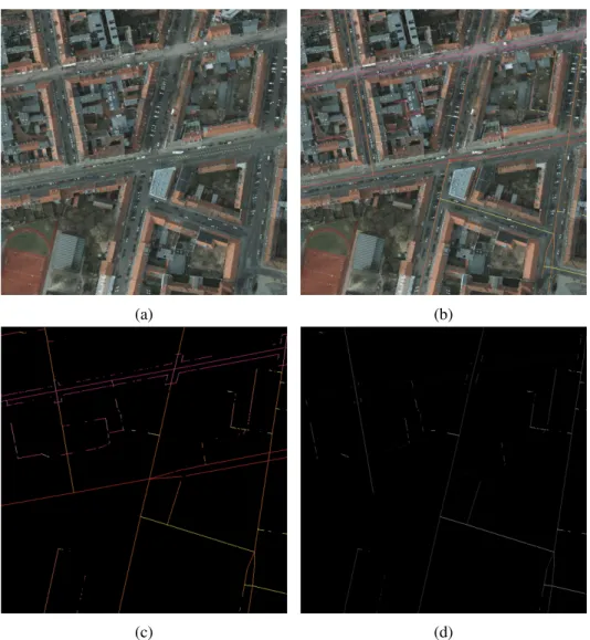
Figure 3.11: Comparison between the proposed technique (a, b, c), DeepRoadMapper [39] (d, e, f), and RoadTracer [3] (g, h, i) for the cities of Pittsburgh (left column), San Diego (middle column), and Kansas City (right column). Green: true positives. Red: false positives. Blue: false negatives. Ground truth: OpenStreetMap [48]. The full resolution comparison results for all 15 cities and the source code can be downloaded fromhttp://theictlab.org/lp/2019Re_X/

on the aforementioned 15 cities with- and without- the proposed post-processing. Furthermore, we applied our processing method on the results of DeepRoadMapper by replacing its own post-processing steps. As it can be seen from the reported metrics the proposed post-post-processing method has a significant and positive effect on the evaluation results. Specifically using our network, in

(39)

Tokyo where the network performs the worst the F1 score increased by30%and IoU increased by 19% when using our post-processing method, while the overall F1 score increased by10%, and IoU increased by 9%. For DeepRoadMapper, the average performance improved by4%on both F1 score and IoU after substituting their post-processing method with ours. It should be noted that DeepRoadMapper uses a post-processing method which relies on training yet another deep neural network to recover the missing segments and connect the gaps in the raw segmentation result. The authors indicate that the training of this second network takes at least a day to reach a good performance score. Thus, the iterative Hough transform method is not only improving the overall performance, but also takes less time to perform the task. All measurements shown in Table 3.2 are based on the F1 score and IoU metrics.

(40)

Chapter 4

Road Extraction using Deep

Reinforcement Learning

Semantic segmentation using deep learning techniques have been developed for many years, and have achieved a very good level in terms of the accuracy of pixel-wise classification, some re-cent works [9, 71] have reached nearly90%mIoU score on the 2012 PASCAL VOC segmentation challenge [20]. The score is 43.1% higher than FCN [35],22.8% higher than the deconvolution network [47]. As for the road extraction task, most researchers are following a similar approach which first performs a semantic segmentation of road pixels and then applies some post-processing techniques to refine the segmentation and extract road boundaries/centerlines. There are three main problems with this kind of workflow:

• Although semantic segmentation is still evolving, the accuracy of road extraction using se-mantic segmentation remains at around60%. So we have a reason to believe that the perfor-mance of road extraction task with the typical "segmentation and post-processing" technique is reaching an upper bound and will be difficult to surpass.

• Current semantic segmentation network architectures can be very confident while looking for the center area of an object, but less confident at the boundaries/edges. Although tricks like skip connections in U-Net and SegNet can help to generate smoother results, boundaries and edges are not as clear as the main body of objects in the final segmentation. But for roads,

(41)

boundaries or centerlines are vital features and more important than the roads surface. Road boundaries or centerlines are often not clear enough or even incomplete in the segmentation results due to convolutional operation itself and also the occlusion of trees and vehicles. • The segmentation result for roads is rasterized and can not be directly used in most of the

real-life applications, so processing is almost always required. There are plenty of post-processing techniques available, but which technique to use usually depends on what kind of segmentation we have. This fact makes the human labor involvement a necessary step during road extraction and thus it can no longer be considered an automatic process.

On the other hand, although reinforcement learning is not a new subject, the application of reinforcement learning can be seldom seen over a long period. Until AlphaGo, an AI Go player developed by Google DeepMind, defeated world top Go player Lee Sedol in a five-game Go match in March 2016, the application of reinforcement learning finally come into the spotlight. The tech-nique behind AlphaGo [58] is actually a combination of reinforcement learning and deep learning, where a deep neural network is used as a decision function. In fact, the work in [44] is the first to apply a deep neural network into the reinforcement learning framework. This was later named deep reinforcement learning, and made it possible for a machine to learn playing Atari 2600 video games at human expert level. More recently, a new AI agent called AlphaStar [65] developed by Google DeepMind successfully mastered on the real-time strategy game StarCraft II, and was able to beat 99.8%of all human players.

In recent years, a few works on applications of reinforcement learning have been done, and most of them focus on self-driving cars or indoor path planning for robots. Considering the drawbacks of semantic segmentation and the advances of deep reinforcement learning, we investigate the use of deep reinforcement learning for the task of road extraction.

4.1 Fundamentals of RL

Reinforcement learning is an area of machine learning which aims at training the learning agent on how to behave (take actions) in a given environment so that it can maximize a cumulative re-ward. Figure 4.1 shows a simple example of a typical environment used to train a reinforcement

(42)

Figure 4.1: CartPole-v1 Environment [4]. This environment consists of a track, a cart that can move along the track, and a pole attached to the cart. the pole is not solid fixed on the cart, in other words, the joint between the cart and pole is un-actuated. The system is controlled by applying a force from the left or the right to the cart. The pendulum starts upright, and the goal for a learning agent is to prevent it from falling over as long as possible. A reward of +1 is provided to the agent for every second that the pole remains upright. The game ends when the pole is more than a certain degrees from vertical, or the cart moves more than a certain length away from the center.

learning agent. A complete reinforcement learning system consists of4component: environment, observation, action and reward. The explanation of these concepts are as follows:

Environmentis the state-space that the learning agent will explore and interact with.

Observationis a sub-space of the whole environment, which is visible to the learning agent at each time. The learning agent will make decisions based on its former experience and current observation.

Actionin an action space that contains all possible actions to take in the environment.

Rewardis gained when learning agent achieves a goal as expected. Can be positive or nega-tive.

Figure 4.2 shows the relationship between these4components. In an environment, the learning agent has an observation. According this observation, an action is taken by the agent. This action can possibly change the settings of the environment, so the environment space is updated after every iteration after the agent takes an action. The agent will receive a reward according to how its action changed the environment, which can be positive or negative. Then the agent will have

(43)

Figure 4.2: Reinforcement learning system. The agent updates the environment with actions, and environment updates the decision policy of the agent with reward.

a new observation in the environment and will adjust its decision policy to achieve higher reward. After many attempts, the agent will finally learn how to interact with the environment in a way that maximizes the final accumulated reward. In some simple cases, such as the Atari game set and even the Go game that the entire game board i.e. state-space is visible to the learning agent during the game play, the observation space is the same as the environment space. But in most cases, they are different. For example in the case of self-driving, the agent is driving a car through a city. The observation is the view captured by a camera/radar sensor in front of the agent. The environment is the entire city, which contains much more context than the observation of the agent.

4.2 Technical Overview

The system takes satellite image tiles as input. An image patch centered at a road pixel is sampled and fed into a deep neural network. The network is used as a decision function and predicts the best action to take at each location. The action is then applied by the learning agent to update the environment and receive rewards. During training, the ground truth is used to check whether all roads in the image are visited and terminates the tracking progress when it is finished. During the inference stage, the ground truth is unknown to the system, thus the termination request will be

(44)

Figure 4.3: RL System Overview. During training progress, the ground truth information will be used to determine whether the agent is on the right track, and also to tell if the terminate state is reached. During inference, the lower part in the figure will be removed, so the agent will trace the road all by itself.

given from other factors in the environment. The output of this system is expected to be a road network in a graph format for each satellite image tile. Figure 4.3 summarizes the reinforcement learning system overview.

4.3 Design the DRL System

To design a reinforcement learning system, we need to define the 4components according to the problem we want to solve. In our case, we want to formulate the problem of satellite image road extraction into a automatic road tracking and exploring task, similar to the process of training a robot to achieve the self-driving task in urban street environment. Based on the characteristics of the problem, we define our RL system as follows:

Environment.At both stages of training and inference a satellite image forms the environment. Once the process starts, the roads that have been visited by the agent will be remembered and labeled, so that the agent will know which road is visited before and which is not.

Observation. For every move of the learning agent, an image patch centered at the current position of the agent is extracted. We set the patch size to200×200to ensure the context visible to the agent is enough to learn the orientation of the current road and make a decision on which direction it will go for the next step.

(45)

Action. For the road tracking problem, we define the actions as moving along the8directions around the agent: north, east, south, west, northeast, southeast, northwest, southwest.

Reward. Starting from a road point in the environment, the agent should keep walking along the road. Every time when the decision made by the agent leads it to a road point that it has not yet visited before, a positive reward will be given. If the decision leads the agent onto a visited road pixel, a small negative reward/penalty will be given to encourage the agent explore more. Finally if the decision leads the agent to go off the road, the agent will receive a great negative reward/penalty. If the accumulated reward keeps decreasing, then this means that the agent keeps tracing along a visited road, or keeps making mistakes by going off the road. When the accumulated reward reached a certain negative number, it will raise a "game over" signal to terminate the current tracing process and reset the environment to start from the beginning again.

One thing that is worth noting is the complex nature of the environment space. Consider the Go game, which uses19×19 grids as its game board and each grid on board has three possible cases (white, black, not occupied), is considered to have a complexity of 10to the power of170 possible board configurations. In our case, the resolution of each satellite imagery is4096×4096 (pixels), and each pixel is represented by [R, G, B] values ranging in[0,255]. The complexity of our environment is intractable. Thus, we first need to simplify our environment.

4.4 Creating the Environment

There are several issues that one needs to consider when creating the environment. On one hand, tracing roads in high resolution satellite imagery has a very high complexity. On the other hand, training an agent to trace the road using deep reinforcement learning always begins from a starting point. The agent then explores the surrounding region and tries to move further away in incremental steps. This makes the size of state-space visible to the network limited. This is in contrast to image classification or semantic segmentation where networks process a batch of randomly sampled patches at every epoch and therefore learn to generalize quickly.

For these reasons, while creating the environment for the designed reinforcement learning sys-tem, we were following two simple rules:

(46)

(a) (b)

Figure 4.4: RL Mesh Envirinment. 4.4a shows mesh only, 4.4b shows road centerline labeled.

• The environment must be as simple as possible to make it easier for the learning agent to optimize its decision policy.

• Since we are training the agent to trace roads in the image, the environment should have a good representation for road/non-road regions.

Following these two rules, the easiest way to simplify the environment is down-sampling the high-definition satellite image to reduce its resolution. A serious problem arises when the image is down-sampled by a large factor: there is a massive loss of information. We found that the general road width in the dataset is around20pixels, and the resolution of the satellite imagery is4096× 4096. If we down-sample the image to one-tenth of its original, the roads in the resulting image will have a width of2pixels. A narrower road in the original image will vanish during the down-sampling process. Thus, we would rather keep the high resolution image as it is, and create another image whose size is one-tenth of the original to be used as the learning environment. A mesh is drawn on each high resolution satellite image, and each grid in the mesh is mapped into a pixel in the small image. By doing so, the small images are considered as the representation of the large one. Figure 4.4a shows an example of the reduced-size image (mesh) environment from a satellite imagery.

(47)

we remove all pixels that are not mapped into road pixels in the original satellite image, and label them as non-road pixels. The rest of the pixels in the environment are labeled as road pixels (as shown in Figure 4.4b). While running the deep reinforcement learning system, the small image is used as the environment that the agent explores in, and the original high resolution image is only used as the input to the deep neural network, which acts as the decision function in the reinforcement learning system.

4.5 Experiments

4.5.1 Environment Configurations

To create the environment, we randomly choose one image tile from the dataset. The image resolu-tion is4096×4096, and ground sampling resolution is60cm. We draw mesh on the image to get the grids, each having a size of10×10pixels. A small single channel image of size409×409is then created. While mapping each grid into a small image we check whether there is road centerline extracted from OpenStreetMap [48] lying through this grid. If there is any, the region in this grid will be labeled as road, and the corresponding pixel in the reduced image (mesh) is labeled as road pixel (use1as its value). Otherwise, the grid is a non-road and the linked pixel in the reduced image is labeled as non-road pixel (use0as its value).

Next, the409×409image is used as the environment. For every training epoch, the agent starts from a randomly selected road pixel. The step size is set to1pixel in the environment (equivalently to10 pixels in the original satellite image). First the current position of the agent in the original satellite image is located, and a patch of size200×200is cropped and fed-forward into the deep neural network. According to the network output, an action is taken by the agent. During the tracing process, if the action leads the agent to a road pixel which is never visited before, a reward of10 points will be given to the agent. If the agent steps onto a road pixel that has been visited before, it will get the small penalty of−1point. Finally, if an action is leading the agent to a non-road pixel, the agent will not move in the environment, and a large penalty of−10points will be given. When all the road pixels in the environment are visited at least once by the agent, this training epoch will end. In addition, if the accumulated reward reaches−500before the agent managed to visit all road