Case study of a sales simulation system
KASPER KARLSSON
TOBIAS LANS
Chalmers University of Technology
Department of Computer Science & Engineering
Computer Science - Algorithms, Languages & Logic
Master of Science Thesis
pose make it accessible on the Internet.
The Authors warrant that they are the authors to the Work, and warrant that the Work does not contain text, pictures or other material that violates copyright law.
The Authors shall, when transferring the rights of the Work to a third party (for ex-ample a publisher or a company), acknowledge the third party about this agreement. If the Authors have signed a copyright agreement with a third party regarding the Work, the Authors warrant hereby that they have obtained any necessary permission from this third party to let Chalmers University of Technology and University of Gothenburg store the Work electronically and make it accessible on the Internet.
BIG DATA ALGORITHM OPTIMIZATION
CASE STUDY OF A SALES SIMULATION SYSTEM
KASPER KARLSSON TOBIAS LANS
c
KASPER KARLSSON & TOBIAS LANS, July 2013.
Examiner: PETER DAMASCHKE
Chalmers University of Technology
Department of Computer Science and Engineering SE-412 96 G¨oteborg
Sweden
Telephone + 46 (0)31-772 1000
When sales representatives and customers negotiate, it must be confirmed that the final deals will render a high enough profit for the selling company. Large companies have different methods of doing this, one of which is to run sales simulations. Such simulation systems often need to perform complex calculations over large amounts of data, which in turn requires efficient models and algorithms.
This project intends to evaluate whether it is possible to optimize and extend an existing sales system called PCT, which is currently suffering from unacceptably high running times in its simulation process. This is done through analysis of the current implementation, followed by optimization of its models and development of efficient algorithms. The performance of these optimized and extended models are compared to the existing one in order to evaluate their improvement.
The conclusion of this project is that the simulation process in PCT can indeed be optimized and extended. The optimized models serve as a proof of concept, which shows that results identical to the original system’s can be calculated within < 1% of the original running time for the largest customers.
We would like to start by thanking Pierre Sandboge for his help with getting the systems up and running and his never-ending patience for our questions.
We would also like to thank Peter Damaschke for acting as our supervisor and making this project possible.
A final thanks goes out to Hoi-Man Lui, Peter Borg and all of the other great people at the Omegapoint office in Gothenburg.
List of Figures iii List of Tables v List of Algorithms vi 1 Introduction 1 1.1 Motivation . . . 1 1.2 Big data . . . 1
1.3 Goals and limitations . . . 2
1.4 Thesis outline . . . 2
2 Simulation 4 2.1 Customer discount simulation . . . 4
2.1.1 Data needed for a customer discount simulation . . . 5
2.1.2 The simulation process . . . 9
2.1.3 Discount inheritance . . . 12
2.1.4 Current implementation . . . 13
2.2 Scaling simulation . . . 17
2.2.1 Data needed for a scaling simulation . . . 18
2.2.2 Discount stairs . . . 20
2.2.3 The scaling simulation process . . . 21
2.2.4 Scaling simulation output . . . 23
2.2.5 Technical difficulties . . . 23
3 Method 24 3.1 Customer Discount Model . . . 24
3.1.1 Preparation step . . . 25
3.1.2 The simulation step . . . 28
3.1.3 Complexity analysis . . . 30
3.2.1 Model overview . . . 33
3.2.2 Calculate constants . . . 34
3.2.3 Prepare scaling node . . . 36
3.2.4 Scaling simulation . . . 38
3.2.5 Database indexing . . . 40
4 Results 41 4.1 Customer discount results . . . 41
4.2 Scaling results . . . 50
5 Discussion 54 5.1 Customer discount simulation . . . 54
5.2 Scaling simulation . . . 56
5.3 Future work . . . 57
5.4 Conclusions . . . 57
2.1 An example article tree containing clothes and accessories . . . 6
2.2 A print screen from PCT showing how simulation output is presented in the current system . . . 10
2.3 An example article tree where discount rates have been set for four nodes 13 2.4 Discount inheritance in the example article tree from figure 2.3 . . . 13
2.5 Redundant calculation of values in PCT . . . 17
3.1 Path tree with aggregated sales history . . . 26
3.2 Propagation of simulated values . . . 29
3.3 Customer discount simulation formulas . . . 29
3.4 Explanation of the complexity variables in algorithm 3.1.4 . . . 31
3.5 Path tree with scaling functionality . . . 33
3.6 Aggregation of order rows for the cache . . . 37
3.7 Overview of scaling simulation procedure . . . 39
3.8 Scaling simulation formulas . . . 39
4.1 Comparison of running time for first simulation between PCT and our model . . . 42
4.2 Running time for repeated simulations over the same datasets in PCT . . 43
4.3 Running time for repeated simulations over the same datasets in our model 44 4.4 Comparison of running time for first simulation between PCT and our model . . . 45
4.5 Running time for first simulation using our model . . . 46
4.6 Comparison of running times depending on the proportion of sales history under the chosen price level 1 node . . . 47
4.7 Comparison of running times where conditions affect the specified number of articles . . . 49
4.8 Running time for scaling simulations where the number of order rows increases . . . 50
4.9 Running time of scaling simulations where the percentage of total sales history used for scaling increases . . . 51 4.10 Correlation between the number of articles that are affected by conditions
2.1 The amount of nodes for each level of the article tree provided for this
project . . . 7
2.2 An example order row from the aggregated sales history database . . . 7
2.3 An example customer condition . . . 8
2.4 The columns which are used to structure the output from a simulation . . 11
2.5 The meaning of different complexity variables in algorithm 2.1.2 . . . 15
2.6 An example order row from the order history database . . . 18
2.7 An example scaling condition . . . 19
2.8 An example set of discount thresholds . . . 20
2.9 The resulting discount intervals from the thresholds in table 2.8 . . . 20
4.1 Running time for first simulation in PCT and our model . . . 42
4.2 Running time for repeated simulations in PCT and our model . . . 44
4.3 Running time for first simulation in PCT and our model over generated data . . . 46
4.4 Running time for different history distributions in PCT and our model . . 48
4.5 Running time depending on the amount of articles covered by existing conditions . . . 49
2.1.1 findDiscountRate(Node n) . . . 12
2.1.2 Structure of the simulation process in PCT . . . 14
2.2.1 getValues(Node na) . . . 21
2.2.2 scalingSimulation(Node na, DiscountStairds) . . . 22
3.1.1 Prepare simulation . . . 27
3.1.2 findDiscountAndDependency(AggregatedSalesHistory art) . . . 28
3.1.3 Customer discount simulation . . . 30
3.1.4 Structure of the prepare simulation step . . . 31
3.2.1 Prepare scaling simulation . . . 34
3.2.2 getValuesAndPathLevel(artAgg) . . . 35
3.2.3 Prepare scaling node . . . 38
3.2.4 Scaling node simulation . . . 38
1
Introduction
1.1
Motivation
Omegapoint is an IT consulting company focusing on business development, high quality system development and information security.
One of Omegapoint’s clients wish to improve and extend their current order system. This system is called PCT, which stands for Price revenue management Client Tool. PCT is used by sales representatives to find suitable discount rates for different items when negotiating with customers. As a central part of this process, a sales representative will run simulations over different discount rates in order to evaluate their expected profit.
When the system performs a simulation, it starts by making an estimation of the customer’s future order quantities based on their order history. This estimation serves as a basis when calculating the expected marginal profit which the given discount rates will yield. However, running such simulations takes too long time in PCT and as such an optimization of the simulation process is needed.
1.2
Big data
Big data is a slightly abstract phrase which describes the relation between data size and data processing speed in a system. A comprehensible definition of the concept is “data whose size forces us to look beyond the tried-and-true methods that are prevalent at that time.” [1]. This means that a scenario where innovative optimization of both models and algorithms is required to handle large amounts of data might well be classified as a big data problem.
In PCT, the big data challenge arises from the huge amounts of data needed in order to run simulations for large customers. In some cases more than fifty thousand historical order rows may have to be handled, with multiple possible conditions and discount rates applied to every single one of them. While the data set itself is not extremely large by
today’s standards, the complex operations and calculations which have to be performed on each one of them adds new dimensions to the simulation procedure. Discounts are for example inherited through a large tree structure containing tens of thousands of nodes and the results must be presented to the user within a reasonable amount of time.
The reasonable time limit has been defined as ten seconds for the simulation proce-dure in PCT. This value is based on research [2, 3] showing that a system user who has to wait even further for results of complex calculations will lose focus - something which could prove devastating during a negotiation with a customer.
An ideal simulation procedure would always return the results within just a few sec-onds, since this would mean that simulations could take place during normal conversation without requiring any waiting at all.
1.3
Goals and limitations
The first goal of this project is to optimize the existing discount simulation algorithm in order to reduce its running time. The discount simulation’s purpose is to apply given discounts to articles and article categories, in order to evaluate whether they will generate an acceptable profit for the selected customer.
The second goal is to create a model with associated algorithms for a scaling extension of the system’s simulation functionality. The purpose of this extension is to make it possible to apply different discount rates depending on the volume of individual orders. This will encourage customers to place a few large orders every year instead of several small ones, thus decreasing shipping and warehouse charges for the company without reducing the sales volumes.
In order to achieve these goals, this report focuses on two possible areas of improve-ment - optimizations of the models and algorithms themselves and improveimprove-ments of the underlying SQL database. Other possible improvements such as hardware upgrades on machines running the algorithm, implementations of the algorithm in programming languages other than Java or other database solutions than SQL are not considered.
1.4
Thesis outline
The rest of this report is divided into four chapters - Simulation, Method, Results and Discussion.
The Simulation chapter begins with a detailed description of how discount rate sim-ulations work and the problems which the current implementation has introduced. The second part contains a specification of the scaling simulation functionality and an expla-nation of the technical difficulties which are introduced by this extension.
The Method chapter describes the models and algorithms which have been developed in this project. It also contains a theoretical analysis of these and comparisons between the current implementation in PCT and our solution.
In the Results chapter, the performance of PCT as well as of our solutions for both the optimized customer discount model and the scaling extension are presented. This
is split up into a set of test cases, with motivations of their relevance for actual usage scenarios.
The report is wrapped up with a Discussion chapter. This is where the results are discussed and conclusions and ideas for future work are presented.
2
Simulation
When a sales representative negotiates with a customer, one can think of it as a sort of balancing problem. The sales representative wishes to maximize the profit gained by keeping discounts at a minimum, while the customer wants to minimize his or her costs by maximizing the discounts. This is where the simulation process comes in handy - by simulating the effects of new discounts, it is possible to decide whether they are profitable enough or not.
When both the sales representative and the customer are satisfied with the results, they can save the discounts as conditions in the system’s database. Discount rates from such conditions will then be applied to the customer’s future orders.
This chapter is divided into two main parts. The first one describes how customer discount simulations work and how these are currently implemented in PCT. The second part focuses on a scaling extension to the simulation process, which makes it possible to use different discount rates depending on individual order volumes.
The models and algorithms presented in this chapter are not necessarily identical to the ones implemented in PCT or the optimized system. They are supposed to be read as explanations of the expected functionality of an arbitrary implementation, unless anything else is explicitly stated.
2.1
Customer discount simulation
Customer discount simulations are currently fully implemented in PCT. By running a simulation over the data described in section 2.1.1, a sales representative will find out which profit would be gained if the customer bought the same articles as in the historical period but using current pricing conditions. Even more importantly, new discount rates can be applied to the simulation meaning that the sales representative can see which effects they will give and whether they seem profitable enough or not.
the chapter in the presented order is highly recommended. Understanding of the under-lying concepts is a great advantage when trying to gain insight into the workings of the simulation process.
2.1.1 Data needed for a customer discount simulation
A simulation is based on data from the following sources:
• Article tree - A tree structure where branch nodes represent article categories and leaf nodes represent articles
• Sales history - A set of aggregated order rows, containing information about pre-vious sales history
• Existing customer conditions - Agreed discount rates from existing contracts, which set a certain discount rate to a specific node in the article tree
• User input - Various parameters that specify which historical data and discount rates to use in the simulation
Since the contents of these data sources are very central to the simulation process, a quick description of each one of them is presented below.
The article tree
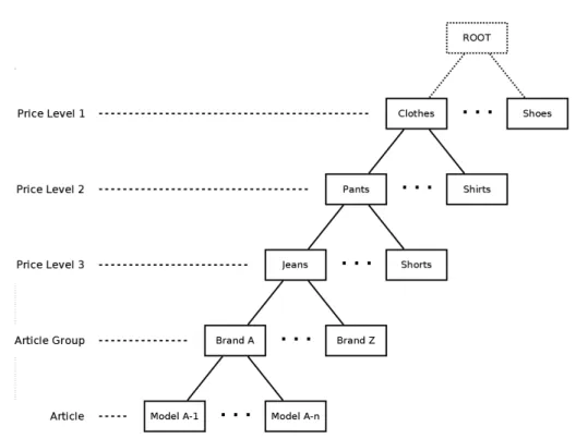
The article tree categorizes all of the company’s articles into article groups. These are in turn grouped together into more general categories in three “price levels”, where level 3 is the most specific and level 1 is the most general category. An example tree using this structure is presented in figure 2.1.
Figure 2.1: An example article tree containing clothes and accessories
As seen in this figure, leaf nodes contain articles while branch nodes represent article categories. The most general categories are stored in price level 1 (Clothes and Shoes), subcategories of these in price level 2 (Pants and Shirts are both subcategories of Clothes) and so on. In the current article database, each price level 3 node contains exactly one article group meaning that these two levels are equally specific.
While the tree in the figure is just an example (using made up names of clothes and accessories instead of the more cryptical category codes from the real system), it should be enough to explain the concept of the article tree structure used in PCT. The amount of nodes for each level in the reduced tree provided for this project is shown in table 2.1. The corresponding numbers for the actual system’s tree are even larger. Since internal company policies do not allow sharing of the full article tree, this reduced tree has been used throughout the whole project.
Node level #Nodes Price level 1 8 Price level 2 64 Price level 3 802 Article Group 802 Article 9,706
Table 2.1: The amount of nodes for each level of the article tree provided for this project
Sales history
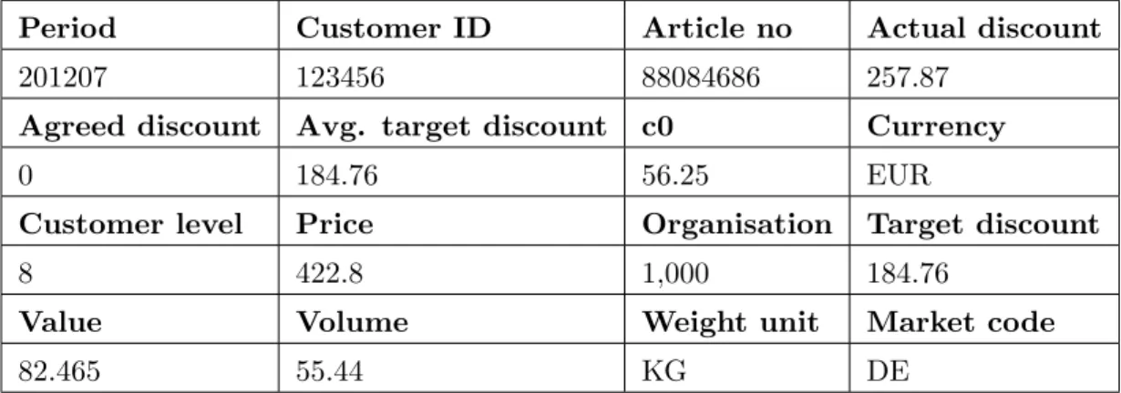
The sales history consists of a database containing a large set of historical order infor-mation, aggregated on a per month basis. An example aggregated order row is shown in figure 2.2.
Period Customer ID Article no Actual discount
201207 123456 88084686 257.87
Agreed discount Avg. target discount c0 Currency
0 184.76 56.25 EUR
Customer level Price Organisation Target discount
8 422.8 1,000 184.76
Value Volume Weight unit Market code
82.465 55.44 KG DE
Table 2.2: An example order row from the aggregated sales history database
This example row shows that customer123456 in the German market bought a total of 55.44 kg of article88084686 during July 2012. One can also see what the total value of the sold articles were, which discount the customer received and so on. The fields which are relevant for the simulation process are described in greater detail in section 2.1.2.
To provide the reader with a perspective of the amount of data stored here, the sales history database for the German market alone stores around 750,000 such aggregated order rows during a single year.
Existing customer conditions
When a sales representative and a customer agree on a discount rate for a certain article or article category, this is added to a database of customer conditions. An example condition is shown in figure 2.3.
ID Opt lock Aggvalorvol Channel
abcdef0123456789 0 01
Command Dirty Discount Eff. stop date
1 FALSE 10.5
Freeze enddate Freeze pl date Freeze start date New freeze FALSE
Note End date Start date Status
This is just an example 201310 201211
Contract ID Created by Customer ID Pricelevel ID
fedcba0987654321 SalesRep01 123456 DEPL3 10
Unfreeze cond. ID
Table 2.3: An example customer condition
In this example, we can see that the sales representativeSalesRep01 has agreed to give customer123456 a 10.5% discount on all articles in the categoryDEPL3 10. Other fields indicate the ID of the condition, the ID of the contract which the condition belongs to, whether or not the condition is temporarily disabled (“frozen”), an optional note specified by the sales representative and so on. Once again, the fields that are relevant for the simulation process are described in greater detail in section 2.1.2.
User input
The final data needed for a simulation is provided by the user. This data consists of a
customer, a path leading from the root down to an arbitrary node in the article tree, a
time period and a set of discount rates for the nodes in the path.
The customer is specified as a reference to the ID of a customer in the customer database. Each sales representative has a set of assigned customers whom he or she can choose from.
The path is as a set of selected nodes in the article tree, where the first selected node lies on price level 1 and any node added afterwards must be a child of the last selected node. This means that there is always a price level 1 node in the path and that the sales
representative may choose to add a price level 2 node as well. If a price level 2 node was added, the user can choose to proceed by adding a price level 3 node and so on. The shortest possible path has the length 1 (meaning that the path consists of a price level 1 node) and the longest possible path has the length 5 (containing one node each from price levels 1-3, an article group node and finally an article node), which is equal to the height of the article tree.
The time period is represented by a start date and an end date, each represented as a combination of a year and a month. When a simulation is run, historical order data whose period parameter lies inside of this interval will be used and any data outside of the interval will be ignored. The end date must of course lie after the start date and the start date must lie within the last 13 months. This limit ensures that a full year’s history can always be used, since the sales history database may not contain the current month’s full history yet.
Finally, the user will specify a discount rate for each node in the path. A discount rate is a decimal number between 0.0 and 99.9 with one decimal value, representing the discount percentage. It is also possible to let a node inherit its parent’s value by not assigning a discount rate to it. Since the price level 1 node does not have a parent node to inherit from, its discount is set to 0.0% if no discount rate is entered on this level. The discount rates are typically modified multiple times during the simulation process, since the sales representative must simulate over multiple configurations in order to find a suitable set of discount rates to add to a contract.
2.1.2 The simulation process
The sales representative starts by entering which customer he is negotiating with and selecting a path in the article tree (see section 2.1.1) for which discounts will be entered. Next up, a start and stop month is specified and now the system is ready to run the first simulation.
Since no discount rates have been entered at this point, all nodes in the path will use their existing discount rates if any such exist in the active conditions and 0.0% otherwise. All price level 1 nodes which are not affected by the existing conditions will also have their discounts set to 0.0%. Due to the concept of discount inheritance (see section 2.1.3), all other nodes will inherit their parent’s discount rate top-down if they do not have an existing condition. This means that the results of the first run will always show the economical results that will follow if the same item quantities are sold as in the historical data used for the simulation, taking only currently active conditions into account.
Conditions may have been added or removed since the historical orders were handled, so it is not enough to just aggregate the values and profits from the history database. Instead, the “base value” (which one can think of as the price for the order rows if no discounts had been applied) must be calculated for each article. By applying discount rates from existing conditions to these base values, the system finds out how much the customer would have to pay for the same orders if they had been placed using current conditions.
In the next step, the sales representative sets discounts for the nodes in the selected path and runs another simulation over the same data. Any conditions affecting discount rates for the path nodes will be overrun by the discount rates set by the sales repre-sentative, while conditions affecting other nodes will still be taken into consideration. The user specified discount rates will then be inherited down through the article tree just like the ones from the conditions. The result will thereby correspond to the profit which would be achieved if these new rates were added to the conditions database and the same orders as in the historical data were then placed again by the customer.
This simulation step will typically be run multiple times with different discount rates for the nodes in the path, until they are balanced in such a way that both the customer and the sales representative are satisfied with the results. Running multiple simulations with different discount rates for the same time period and historical data until one gets satisfying results is referred to as going through a simulation process.
Simulation output
So far, the output of simulations has been described in terms of “profit” and “value”. The actual values computed during a simulation are of course more specific than that and as such, the specification of requirements presents guidelines for the output data layout.
The specification indicates that the output should be presented as a table, where each node in the selected path is represented as a row. There is also a top row labeled “Total”, which shows the total simulation values of all articles in the whole article tree.
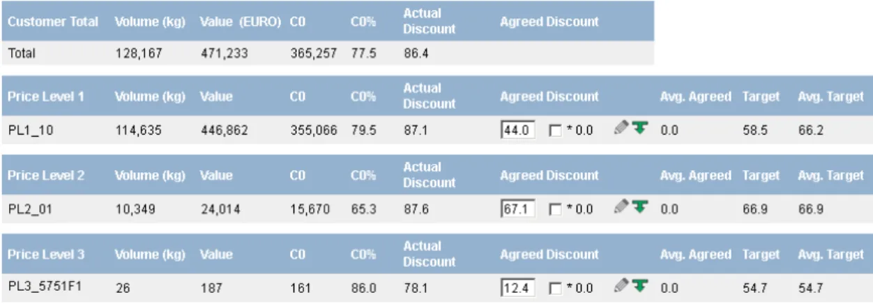
A print screen showing how this looks in the current version of PCT is shown in figure 2.2. The columns of each row are described in table 2.4.
Figure 2.2: A print screen from PCT showing how simulation output is presented in the current system
Field name Unit Type Description
Node name n/a String The name of the row’s node
Volume kg Integer The total volume of all orders for articles under the row’s node in the article tree Value Euro Integer The total amount of money which the
customer would have to pay if all historical orders for articles under the row’s node were placed again, with the new discounts applied C0 Euro Integer The profit which the company would gain if
all historical orders for articles under the row’s node were placed again, with the new discounts applied
C0% Percent Decimal Shows how many percent of the row’s value number C0 corresponds to, i.e. (Value/C0)*100 Actual discount Percent Decimal The average historical discount for articles
number under the node in the simulation period Above target n/a Boolean A warning flag which shows whether the
agreed discount is higher than the node’s target discount
Agreed discount Percent Decimal The discount used for the row’s node in number the current simulation
Avg Agreed Percent Decimal The average agreed discount for articles number under the row’s node in the article tree Target discount Percent Decimal A recommended target discount for the node,
number based on the customer’s pricing level Avg Target Percent Decimal The average historical target discount of
number articles under the row’s node
Table 2.4: The columns which are used to structure the output from a simulation
The five last columns are empty for the “Total” row, since these values are considered irrelevant to display for the whole article tree.
2.1.3 Discount inheritance
Discounts can be applied to nodes on any level of the article tree - from price level 1 down to specific articles. It is intuitive that a discount which is set for a single article will only affect the price of that specific article. When it comes to discounts set on article groups or price level nodes, the system uses a concept called “discount inheritance” to let this affect underlying nodes. In order to determine which discount rate to apply to a given node, the method presented in algorithm 2.1.1 is used.
Algorithm 2.1.1: findDiscountRate(Node n) Input: A noden from the article tree
Result: The discount rate which should be applied to n
if nis a node in the path for which a discount rate d is set then
1
return d
2
else if n is not a node in the path AND nhas an active condition c then
3
return the discount rate from conditionc
4
else if n is a price level 1 node then
5
return 0.0%
6
else
7
parent := n’s parent node in the article tree
8
return findDiscountRate(parent)
9
end
10
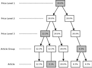
The concept of discount inheritance is easy to visualize due to the tree structure of the article database. An example tree with some existing discount rates is shown in figure 2.3. Existing discount rates are written directly onto the grey nodes to which they belong, while nodes without such rates are white. The final result of the discount rate inheritance in the same tree can be seen in figure 2.4, where arrows show how discount rates are passed down through the tree.
Figure 2.3: An example article tree where discount rates have been set for four nodes
Figure 2.4: Discount inheritance in the example article tree from figure 2.3
2.1.4 Current implementation
As mentioned in the project motivation in section 1.1, the current implementation of PCT suffers from critical performance issues. Since the source code of this system is not allowed to be included in this report, the problems of its algorithm have to be explained in terms of bad structure choices and complexity rather than examples and excerpts from the actual code.
A (very) rough outline of the algorithm structure used to perform simulations in PCT is presented in algorithm 2.1.2. While it does not motivate or explain the details of each step, it does provide enough information to analyse its complexity. To give the reader some sort of idea of the actual magnitude of the implementation of this algorithm, its Java source code takes up several hundred kilobytes (not including GUI, server connec-tions, database handling and other parts which are not directly related to the algorithm). In other words, a line describing e.g. criteria matching means running a separate algo-rithm which in turn has a complexity worth mentioning.
Algorithm 2.1.2: Structure of the simulation process in PCT if this is the first run of the simulation process then
1
initialize connection to each input data element in the GUI [O(k)]
2
end
3
foreach price level in the article tree[O(k)]do
4
match condition level [O(k)]
5
match price level [O(k)]
6
foreach item in the customer’s cache [O(n)]do
7
match criteria [O(k)]
8
end
9
retrieve target discount [O(k)]
10
foreach article in the article tree [O(a)]do
11
foreacharticle in the customer’s cache [O(n)] do
12
match criteria [O(k)]
13
foreachprice level in the article tree [O(k)]do
14
retrieve data and calculate results
15
end
16
end
17
retrieve agreed discounts [O(k)]
18
compare discounts to target discounts [O(k)]
19
end
20
end
21
foreach article in the customer’s cache [O(n)] do
22
calculate results for articles under price level 1 nodes ∈/ path
23
end
24
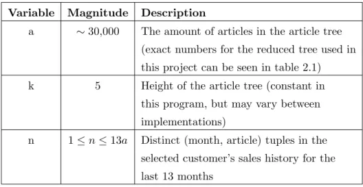
In the pseudo code above, the complexity has been included on each line whereO nota-tion is applicable. The meaning of each occuring variable in theOnotation is presented in table 2.5.
Variable Magnitude Description
a ∼30,000 The amount of articles in the article tree (exact numbers for the reduced tree used in this project can be seen in table 2.1) k 5 Height of the article tree (constant in
this program, but may vary between implementations)
n 1≤n≤13a Distinct (month, article) tuples in the selected customer’s sales history for the last 13 months
Table 2.5: The meaning of different complexity variables in algorithm 2.1.2
The total complexity of the implementation of the current simulation algorithm is
O(k+k(k+k+nk+k+a(n(k+k))+k+k)+n) =O(k+5k2+nk2+2ank2+n) =O(ank2)
It should also be noted that the complexity of repeated runs of the algorithm is
O(k(k+k+nk+k+a(n(k+k)) +k+k) +n) =O(5k2+nk2+ 2ank2+n) =O(ank2)
This is barely an improvement from the first run at all - one single k term is removed since the initialization step on line 2 does not need to be run again. The total complexity of O(ank2) is high in itself, since both a and n can hold quite large numbers and the
k term is used at multiple places. However, this is not the only reason behind the high running times of the algorithm.
Another big problem is the on-demand usage of database resources. Every time a set of values from the database is needed, a new connection to the database is opened. The sought values are then retrieved by an SQL query and afterwards the database connection is closed again. Repeatedly opening and closing database connections takes time and this is done in many parts of the algorithm, including the data retrieval methods mentioned in line 15. This means thatO(ank2) database connections and SQL queries may have to be opened and run in the worst case. Some values are even retrieved from the database multiple times during a single execution, since they are used in multiple places in the code but are not saved after being retrieved the first time.
It should however be noted that some actions have been taken in order to reduce the amount of data retrieved from the database per simulation. Every customer’s order his-tory for the last year is stored as a list in a hash map indexed by the customer ID, which thereby works as an in-memory database. This makes retrieval of a customer’s historical
data (without direct database access) in O(1) time possible. Of course, iterating over the resulting list will still take O(n) time. This cache is created on server startup and updated regularly, so creation and updates of the cache do not affect the running time of the simulation algorithm. Some loops in PCT are still performed over all distinct values in certain database tables when information from this cache could have been used instead, leading to even more unnecessary database lookups.
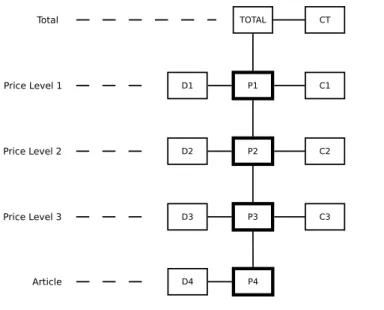
A third cause of the high running time is the redundant calculation of certain values. The foreach loop on lines 4-21 in the algorithm above runs once for each price level and calculates the results for all articles under the node on that level. This means that the results for all articles under the price level 1 node will be calculated first, followed by a recalculation of all articles under the price level 2 node and so on for a total of up to k
calculations of the same values for some articles.
Let the selected path in the simulation be called P and the path from an arbitrary article a up to its price level 1 ancestor be called Pa. Then, |PTPa| (the amount of
nodes which are both inP and in Pa) equals the number of times articlea’s results has
to be calculated during each simulation. Calculating the same value more than once is of course redundant and adds unnecessary running time. This is visualised in figure 2.5. Nodes in the path P are marked with thick outlines in the figure. Values for articles within the blue box (A1−A5) are calculated once, while articles within the green box (A1−A4) are calculated once more and articles within the red box (A2,A3) yet another
time. The purple box (A6) marks articles that lie under a price level 1 node∈/ P, whose
TOTAL Price Level 1 Price Level 2 Price Level 3 Article Group Article A1 A2 A3 A4 A5 A6 P1 P2 P3
Figure 2.5: Redundant calculation of values in PCT
The combination of a high time complexity, inefficient database usage and redundant calculations cause the running time of each simulation to grow rapidly for increasing values ofn.
2.2
Scaling simulation
As mentioned in section 1.1, the company wants a scaling extension of the simulation process and conditions in PCT. The purpose of this extension is to make it possible to apply different discount rates depending on the volume of each individual order. If larger order volumes are rewarded with higher discounts, customers will be more likely to place large orders a few times per year instead of small orders every week or month, thus decreasing shipping and warehouse charges.
The extension’s specification is built around a concept called “discount stairs”. These are set by sales representatives on a per customer and node basis, in order to define which discount rates will be applied to orders of certain volumes. This concept is described in greater detail in section 2.2.2. The data sources which are needed for scaling simulations are in turn described in section 2.2.1.
2.2.1 Data needed for a scaling simulation
A scaling simulation is based on data from the following sources:
• Article tree - A tree structure where branch nodes represent “price levels” (article categories) and leaf nodes represent articles
• Sales history - A set of order rows, containing information about previous sales history. The aggregated sales history from the customer discount model is also required.
• Existing scaling conditions - Agreed scaling conditions from existing contracts, which set a certain discount stair to an article, article group or price level 3 node in the article tree
• User input - Various parameters that specify which historical data to use, which discount stair to use and various other simulation settings
The article tree
This is exactly the same tree as the one used for customer discount simulations, which is described in section 2.1.1.
Sales history
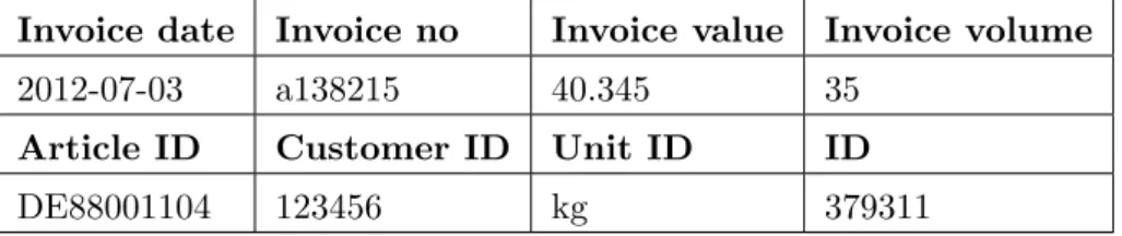
The sales history used for scaling simulations consists of a database containing a large set of historical orders. Note that these order rows are not aggregated, as opposed to the ones used for customer discount simulations. An example order row is shown in table 2.6.
Invoice date Invoice no Invoice value Invoice volume
2012-07-03 a138215 40.345 35
Article ID Customer ID Unit ID ID
DE88001104 123456 kg 379311
Table 2.6: An example order row from the order history database
However, in some situations data from the aggregated database table (described in sec-tion 2.1.1) is used as well. This means that scaling simulasec-tions require both of these database tables to be present.
Existing scaling conditions
Agreed discount stairs for specific article tree nodes and customers are added to a database of scaling conditions. An example scaling condition is show in table 2.7.
Price level ID Customer ID v0 v1 v2 v3 v4
DEP L3 5690F1 123456 5 10 20 30 50
v5 d0 d1 d2 d3 d4 d5
12.1 15.0 17.5 20.0 25.3
Table 2.7: An example scaling condition
In this example, the scaling condition covers the price level 3 node DEP L3 5690F1 for customer 123456. The stair has five thresholds, whose volume limits are shown in columns v0−v4 and their respective discounts in columns d0−d4. Since there is no sixth threshold in this example, v5 and d5 are left empty. A description of how these values are used in a scaling simulation is presented in section 2.2.3.
According to the scaling extension specification, all customers can be expected to have a total of at most ten active scaling conditions. Most discounts are in other words still expected to be handled through customer discount conditions when the scaling extension has been implemented.
User input
The final data needed for a scaling simulation is provided by the user. This data consists of acustomer, atime period, a node and a discount stair.
The customer is a reference to the ID of a customer in the customer database, just like in customer discount simulations.
The time period is represented by a start date and an end date, which is slightly different from the time period in customer discount simulations. Since the historical order rows used for scaling simulations are not aggregated per month like the ordinary order history, these dates specify a day of the month as well.
The node is a reference to either an article, an article group or a price level 3 node in the article tree. This is quite different from the path used in customer discount simulations - not only because only a single node is selected, but also because price level 1 and price level 2 nodes can not be used.
A discount stair is a way of defining different discount rates for the same node, depending on individual order volumes. This is described in greater detail in section 2.2.2.
2.2.2 Discount stairs
As mentioned in section 2.2.1, discount stairs make it possible to apply different discount rates for orders depending on their volumes. Just like in customer discount simulations, discount inheritance (see section 2.1.3) is applied. However, scaling conditions can not be set for price level 1 or price level 2 nodes in the article tree. The reason behind this is that articles who do not share the same ancestor on price level 3 are generally considered too diverse to share volume limits. In other words, it would not always make sense to apply the same discount rate for i.e. orders between 20 and 25 kg on two articles of very different types.
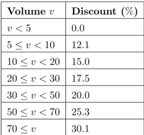
A discount stair consists of between one and six volume thresholds and a discount rate for each one of these. The thresholds indicate boundaries between weight intervals, meaning thatithresholds definei+1 intervals. A set of such thresholds is shown in table 2.8 and its resulting interval limits are shown in table 2.9. Since there are six thresholds in this example, there are seven discount intervals.
Threshold volume Threshold discount (%)
5 12.1 10 15.0 20 17.5 30 20.0 50 25.3 70 30.1
Table 2.8: An example set of discount thresholds
Volume v Discount (%) v <5 0.0 5≤v <10 12.1 10≤v <20 15.0 20≤v <30 17.5 30≤v <50 20.0 50≤v <70 25.3 70≤v 30.1
From the last table we can easily see that an order with e.g. volume v = 4 would get 0.0% discount if this stair is used, while an order with volumev = 27 would receive a 17.5% discount.
2.2.3 The scaling simulation process
The general workings of scaling simulations are similar to those of customer discount simulations, but some differences are of course present. A scaling simulation begins with a sales representative selecting a customer. In excess of this, a price level 3 node, article group node or article node in the article tree (see section 2.1.1) is selected and a time interval specified. Furthermore, a set of one to six volume thresholds is specified. Note that only volumes are entered before the first run - actual discount rates for these are not entered until later. The system is now ready to run the first scaling simulation.
During the first run, the selected node n will use the discount rate 0.0% for each volume interval specified in the input step. After each run, the user can modify the discount rates for each interval of n’s discount stair, apart from the lowest one which is always locked to 0.0%. The values for all articles are calculated according to the method described in algorithm 2.2.1.
Algorithm 2.2.1: getValues(Nodena)
Input: An article nodena from the article tree
Result: Total simulated cost, value and volume for article na
current := na
1
repeat
2
if current is the selected simulation node with discount stair ds then
3
returnscalingSimulation(na,ds)
4
else if current has an existing discount stair da in a scaling condition then
5
returnscalingSimulation(na,da)
6
end
7
current := current’s parent in the article tree
8
until current is a price level 3 node
9
return Total cost, value and volume from aggregated (i.e. not scaling) history
10
database for na during selected time period
As line 10 in the algorithm above shows, values for articles that are not affected by the scaling node or scaling conditions are retrieved directly from the aggregated database table (which is also used for customer discount simulations). This works since the ag-gregated data for a month per definition equals the sum of all individual orders from the same month.
Even if only a part of the month is covered by the selected time interval for the simulation, the whole month’s history will still be used in this case. It should also be noted that the calculation of base prices and application of customer discounts are ignored - the aggregated values are used directly in order to lower the scaling simulation’s
complexity.
Algorithm 2.2.2 shows how the scalingSimulation() function which is called in algo-rithm 2.2.1 works.
Algorithm 2.2.2: scalingSimulation(Node na, DiscountStairds)
Input: An article nodena from the article tree and a discount stairds
Result: Simulated values (cost, value and volume) for article na
totalCost := 0 1 totalValue := 0 2 totalVolume := 0 3
orderRows := all order rows from the scaling sales history (see section 2.2.1) for
4
articlena within selected time period
foreach row r in orderRows do
5
rowVolume := r’s volume
6
aggrPrice := price for na inr’s month in the aggregated history database
7
aggrCost := cost for na inr’s month in the aggregated history database
8
aggrVolume := volume for na inr’s month in the aggregated history database
9
listPrice := aggrPrice / aggrVolume
10
listCost := aggrCost / aggrVolume
11
rowDiscount := The discount fromdswhose volume interval covers rowVolume
12
rowCost := rowVolume * listCost
13
rowValue := rowVolume * listPrice * (1 - rowDiscount*0.01)
14
totalCost := totalCost + rowCost
15
totalValue := totalValue + rowValue
16
totalVolume := totalVolume + rowVolume
17
end
18
return (totalCost, totalValue, totalVolume)
19
Since the specification of historical order rows does not include any columns for price and cost, these values have to be calculated from the aggregated historical data. First off, the article’s “list price” and “list cost” are calculated as a sort of base values on the form currency unit/volume unit (e.g. Euro/kg) for the specified article and month. These values are then multiplied by the current order row’s volume in order to get its price and cost.
Next up, the row’s simulated value is calculated. The row’s volume is matched to a volume interval in the discount stair (as seen in section 2.2.2) and the corresponding discount is applied to the row’s price in order to find its value.
Finally, the sum of all row’s costs, values and volumes are returned. The simulation results are obtained by aggregating the resulting values for all articles, including the ones where values are retrieved from the aggregated historical database.
2.2.4 Scaling simulation output
The output of a scaling simulation should be presented just like the output of a customer discount simulation, which is described in section 2.1.2. The bottom row covers the scaling node, all of its ancestor nodes have a row each in the middle and the top row contains the total values for the whole article tree.
2.2.5 Technical difficulties
Scaling simulations have not yet been implemented in PCT. Adding this functionality has been considered impractical, since scaling simulations run over far larger data sets than customer discount simulations (which already have problems with high running times). The non-aggregated data is even too large to be held in an in-memory database cache, which means that every historical order row will have to be retrieved from an ordinary database. This slows down the data handling even further.
Customers are estimated to place orders for the same article up to once a week and the time period used for a scaling simulation can be at most one year. This means that one can assume a maximum of 52 order rows per article in a single scaling simulation.
As shown in table 2.1, the reduced article tree contains 9,706 distinct articles while the full article tree has around 30,000 nodes. It is deemed possible that a single customer buys up to a thousand different articles regularly.
Scaling simulations can only be run over article nodes or price level 3 nodes in the article tree, but if scaling conditions are specified for other such nodes than the selected scaling node, these require separate scaling simulations on their own. The running time of a scaling simulation over an arbitrary node for a customer will thereby increase for every scaling condition added for the same customer. Price level 3 nodes have an average of 12.3 and a maximum of 172 underlying articles, so adding a single condition could increase the number of required historical order rows by almost 9,000.
This means that running a scaling simulation can require multiple separate scaling simulations for articles with existing scaling conditions. In total, these could require computations over as many as 52,000 historical order rows.
3
Method
This chapter explains the optimized models and algorithms which we have developed during this project. Just like the previous chapter, this is divided into two parts. The first part shows how the customer discount model can be optimized and the second part describes an efficient model for scaling simulations.
3.1
Customer Discount Model
If we examine the current simulation process described in section 2.1.2 and remember the issues from section 2.1.4, we note that the major bottlenecks in the existing imple-mentation are that:
• Simulations suffer from a high time complexity
• Data retrieval from the database and in-memory cache is done in an inefficient way
• The same data is redundantly calculated and aggregated several times in the sim-ulation process
Intuitively, a good place to start in order to reduce the time complexity is to eliminate redundant calculations in the simulation process. Doing this would not only improve the performance of single simulations, but also lead to shorter running times for repeated simulations. An example of this is to save the parts that remain constant during repeated simulations, in order to avoid reaggregation and recalculation of the same values in each run.
Apart from the three bottlenecks there is another issue which can be addressed, i.e. the structure of the article tree. From table 2.1 we can see that there is an equal number of price level 3 and article group nodes in the article tree. As one might suspect, each price level 3 node categorizes exactly one article group. This means that the article
group level does not fill any function and can be entirely removed from the article tree. The resulting article tree will as such consist of four levels, i.e. price level 1-3 and the article level.
A rough outline of our optimized model is to first construct a path tree, where we aggregate parts of the sales history prior to actually performing any simulation calcu-lations. Since we know which articles will be used in the simulation process after the simulation path has been selected, it is a simple matter to tag the articles whose values will remain constant and the ones which will be affected by the simulation. This means that we only need to iterate over the articles in the article tree once. After this, it is a simple and relatively fast procedure to apply the user set discounts and merge the results of the simulation. In order to avoid redundancy, we will use a bottom up approach to merge the results of the simulations.
Our solution consists of two major parts. In the first step, we perform the expensive part of tagging and aggregating the data needed for the simulation. In the second step we perform a small series of calculations on the aggregations to run the simulations and merge the results.
3.1.1 Preparation step
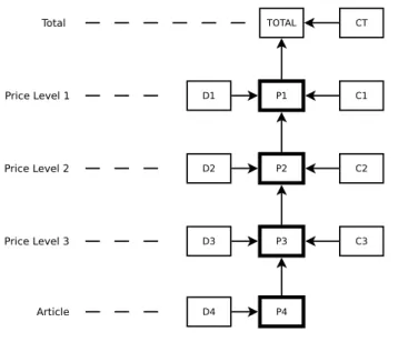
The preparation step consists of retrieving the sales history for the selected customer and time period and merge this with the existing article tree to construct a path tree, which is shown in figure 3.1. Here all the necessary data for the simulation will be aggregated without any user specified discounts applied. This means that we can apply the discounts and calculate the results in a later procedure.
This new tree structure consists of the selected simulation path nodes with dependent and constant parts attached to each node. The dependent part contains the values of ar-ticles under the path node that will be directly affected by the discount set at that node. Respectively, the constant part contains the values of articles under the path node that will remain constant regardless of the discount set at the node. This includes articles that lie under another price level one node and articles covered by existing conditions. In the figure we note that the total level does not have a dependent part, since we can only simulate up to price level one. Similarly, the article level does not have a constant part since articles cannot have any underlying nodes.
TOTAL
Price Level 1
Price Level 2
Price Level 3 Total
Node in chosen path Constant part on level n Dependent part on level n P1 P2 P3 Pn C1 C2 C3 Cn Dn CT D1 D2 D3 Article D4 P4
Figure 3.1: Path tree with aggregated sales history
The aggregation of the relevant history from the in-memory cache into the correct de-pendent or constant node in the path tree is described in algorithm 3.1.1.
By aggregating the customer’s historical data from the PCT cache (which was de-scribed in section 2.1.4) into a temporary customer cache, a smaller set of historical rows is obtained without affecting its total values. The idea here is to have the order history aggregated for each article and customer on a time period basis. This is a big improvement from the original solution, since we can now access the total aggregated sales history for an article in constant time. Previously, this would have required itera-tion through the customer’s entire sales history each time data for an article was needed. We also created a cache for all of the conditions for the selected customer, in order to make fast lookup of discounts from conditions possible.
Algorithm 3.1.1: Prepare simulation
Data: An empty path tree treepath with the same number of levels as specified from user input
Result: treepath populated with aggregated sales history
history populated with all sales history for the selected customer and time period
conditions populated with all conditions that exist for the selected customer
Construct and populate a hash map history that contains aggregated sales history
1
for the selected customer and time period, with the article number as key Construct and populate a hash mapconditions that maps nodes in the article
2
tree to existing conditions for the customer foreach AggregatedSalesHistory art in historydo
3
(index,isConstant,discount) := findDiscountAndDependency(art)
4
current := chosen path node at level index intreepath
5
if isConstant then
6
constVal := applydiscount to sales history for art
7
addconstVal tocurrent’s constant node
8
else
9
add sales history forart tocurrent’s dependent node
10
end
11
end
12
The function call to findDiscountAndDependency that is used in algorithm 3.1.1 finds which node in the path tree to add the article’s sales history to and which discount to apply. This is done by traversing the original article tree upwards from the article, examining if there are any conditions present for the current node in each step. For each article there are three possible outcomes:
• The article’s discount is dependent on a node in the simulated path
• The article is in another price level 1 subtree without a condition
• The article’s discount is inherited from an existing condition
When the article’s discount depends directly on the simulated path, we simply aggregate the sales history into the correct dependent node in the path tree. We don’t have to find a discount in this case, since we will use the one specified by the user. If the article is in another price level one subtree and we do not have a condition specified, we aggregate the sales history to the total constant node with a discount of 0%. Finally, if the article’s discount depends on a node with a specified condition we begin by finding the condition and retrieving its discount. We then locate the path node which this constant article’s data should be aggregated to. Pseudo code for this is presented in algorithm 3.1.2.
Algorithm 3.1.2: findDiscountAndDependency(AggregatedSalesHistory art) Input: Aggregated sales history for an article art
Result: Returns a tuple consisting of
• the discount that should be applied to the article
• a boolean indicating whether the article is constant
• the level in the path tree whichart should be added to
discount := 0.0
1
isConstant := false
2
foreach node n in the path in the article tree from art to price level 1 do
3
for ifrom 1 to 5 do
4
if n equals the node at level i in path tree then
5 return (i,isConstant,discount) 6 end 7 end 8
if n has an existing condition in the conditionshash map then
9
discount := existing condition ofn
10 isConstant := true 11 end 12 end 13
/* Node lies under a price level 1 node outside of the path */ return (0, true, 0.0)
14
3.1.2 The simulation step
After running the preparation step, the heavy computations have been performed and all that remains is to apply the discounts to the dependent nodes and merge the results. We apply a bottom up strategy as shown in figure 3.2, where arrows show how values propagate upwards in the path tree. This is far more efficient than calculating from the top down, as was the case in PCT (see section 2.1.4).
TOTAL
Price Level 1
Price Level 2
Price Level 3 Total
Node in chosen path Constant part on level n Dependent part on level n P1 P2 P3 Pn C1 C2 C3 Cn Dn CT D1 D2 D3 Article D4 P4
Figure 3.2: Propagation of simulated values
The simulation calculations consist of applying the discount from the path node to the data values in the dependent node and calculating the values specified in table 2.4. The next step is to add the values from the constant and child nodes to the simulated dependent value and reiterate this process for each path node until the total level is reached. A high level description of the propagation of the simulated values and the mathematical formulas used to perform these calculations are shown in figure 3.3.
V4 = d4(D4) Vi The values of path node i
V3 = d3(D3) +C3+V4 di(Di) The discount applied to dependent of node i
V2 = d2(D2) +C2+V3 Ci The constant values of node i
V1 = d1(D1) +C1+V2 VT = CT +V1
Figure 3.3: Customer discount simulation formulas
Algorithm 3.1.3: Customer discount simulation Data: A populated path tree
Result: Calculates the values of all simulation path nodes
foreach node n in the simulation path tree from lowest to highest level do
1
if n is on lowest level in path then
2 child := null 3 constant = null 4 else 5
child := path node on the next level
6
constant =n.constant
7
end
8
if n is on highest level in path then
9
dependent := null
10
else
11
dependent := n.dependent with n’s discount applied
12
end
13
calculate n.values based onconstant,dependent and child
14
end
15
To summarize the customer discount model, we have made four major changes to the original model from PCT. The first is that we perform all of the data aggregation from the in-memory cache in a prepare step and aggregate the data from each article into the correct node in the simulation path. The second change is that the path tree is also stored between simulations to allow for faster repeated simulations. The third one is that article groups have been removed from the article tree. The last change is that we merge the results of the simulations in a bottom up fashion, in order to remove the redundancy caused by recalculation of values for each level in the path.
3.1.3 Complexity analysis
In section 2.1.4 we performed a complexity analysis of the PCT implementation. In order to get an idea of how this model relates to PCT, we will perform a complexity analysis of our model as well and compare them. Since the preparation step is where the heavy calculations occur in our model, it is most suitable to compare the complexity of that part to the original model. A very rough outline of the preparation step’s complexity in our model is given in algorithm 3.1.4.
Algorithm 3.1.4: Structure of the prepare simulation step Build article cache [O(n)]
1
Build condition map [O(c)]
2
foreach article in article cache[O(u)] do
3
foreach price level in path from article to price level 1 [O(k)]do
4
Find discount from possible existing condition
5
end
6
Find path node to aggregate article to [O(k)]
7
end
8
Calculate initial values [O(m)]
9
Set target and agreed discounts [O(k)]
10
The pseudocode above contains the complexity in O notation on each line where it is applicable. A description of each variable is presented in table 3.4.
Variable Magnitude Description
a ∼30,000 The number articles in the article tree (exact numbers for the reduced tree used in this project can be seen in table 2.1) k 4 Height of the article tree
n 1≤n≤13a Distinct (month, article) tuples in the selected customer’s sales history for the last 13 months
c <50 The number of active conditions for the selected customer
m 1≤m≤k The height of the selected simulation path u 1≤u≤a The number of distinct articles in the customer’s
sales history for the selected period
From algorithm 3.1.4 we can deduce that the complexity for the preparation step is
O(n+c+u(k+k) +m+k) =O(n+c+ 2uk+m+k) =O(uk)
Once the preparation step has been executed, simulations will have a complexity of
O(m). The analysis of the original implementation in section 2.1.4 showed that the time complexity for each simulation in PCT is O(ank2), where ais the number of articles,n
is the number of articles with sales history and k is the height of the article tree. The complexity is the same both for single and repeated simulations in PCT.
By comparing the complexity of the preparation step in our model to PCT, we can see that there is a factor ofO(nk) difference in favor of our model. In repeated simulations there is a difference of factorO(ank), sincemis bounded byk. This means that at least in theory, our model should work significantly faster than PCT.
3.2
Scaling model
As we saw in section 2.2, the scaling functionality requires an extension and a restructur-ing of the existrestructur-ing simulation procedure. There are however several aspects that remain the same from the customer discount model. The user will still have to choose a path in the article tree to simulate over and it must be possible to run repeated simulations over the same chosen path. Discount inheritance still applies, with the difference that we now have to apply a discount stair (see section 2.2.2).
In order to organize the results, we can reuse the path tree from figure 3.1. This method has already proven efficient in the customer discount model and could as such be used to make quick repeated simulations possible in the scaling model as well.
The main difficulty of the scaling feature is that we now need to work with individual order rows instead of using data aggregated on a per month basis. This means that we can no longer rely solely on the in-memory cache, but that we rather have to retrieve most of the data needed for a simulation directly from the database. The reason for this is that the scaling simulation applies different discounts based on the volume of each specific order row and that this data is too large to be kept in a cache.
Since it is generally slower to read from disk than from memory, one bottleneck in this model is the number of accesses to the database. This means that two of the main optimization goals are to improve the performance of the database and to minimize the number of accesses to it.
As the specification dictates, we can only have one scaling node in a scaling simu-lation. Articles that do not depend directly on this node can be treated in the same way as constant article values were treated in the customer discount model. Since the dependent nodes in the path tree have been replaced by this single scaling node, the path tree used in the scaling model will have the structure shown in figure 3.5.
TOTAL
Price Level 1
Price Level 2
Price Level 3 Total
Node in chosen path Constant part on level n Scaling node P1 P2 P3 Pn C1 C2 C3 Cn S CT Article S
Figure 3.5: Path tree with scaling functionality
3.2.1 Model overview
Since the new functionality demands an extension of the old model, we can originate from our optimized customer discount model. We then need to modify some of its steps and add some new features. The scaling model consists of these three steps:
• Calculate the constant values of the article tree
• Perform precalculations for the scaling node
• Run a simulation over the scaling node
The constant values can be calculated in a manner similar to the prepare simulation step from the customer discount model. The main difference is that scaling conditions are used instead of customer conditions.
The primary idea of the precalculation step is to create an on-demand cache, which will hold all of the order rows needed for a scaling simulation over the scaling node. This new cache will then be used to speed up repeated simulations when the step volumes are changed between runs. After the step volumes have been set, the order rows will be aggregated into the correct step in preparation for an actual simulation. When the discounts in the discount stair have been set as well, a simulation can be run in close to no time in a fashion similar to the method from the customer discount model. This means that repeated simulations with the same step volumes will have very low running times.
3.2.2 Calculate constants
The constant calculation step is quite similar to the preparation step used in the cus-tomer discount model. We iterate over each article in the in-memory sales cache for the selected customer and aggregate the article’s values to the correct path node in the path tree. The difference is that we ignore the articles that are used in the scaling part of the simulation, because we need to use the individual order rows of these articles. The basic outline of the simulation preparation is shown in algorithm 3.2.1.
Algorithm 3.2.1: Prepare scaling simulation
Data: An empty converted tree treepath with the same number of levels as specified from user input plus one for the “Total” level
Result: treepath populated with aggregated sales history with discounts applied
conditions populated with all scaling conditions that exist for the selected customer
Construct a hash map history that will contain aggregated sales history for the
1
selected customer and time period with the article number as key
Construct a hash map conditions that contains the discount stairs for the nodes
2
that have scaling conditions with the node as key foreach AggregatedSalesHistory art in historydo
3
(values,pathlevel) = getValuesAndPathLevel(art)
4
current := node at pathlevel intreepath
5
add values to current’s constant node
6
end
7
prepareScalingNode()
8
The algorithm described above is very similar to the one that we saw in the customer discount model, but with one major difference. In the customer discount model, the calculation of the constant parts was a simple and fast method where the discount could be retrieved from the condition and then applied to the aggregated data. However, using scaling conditions is not that straightforward.
As we saw in section 2.2.2, a scaling condition consists of a scaling stair where the discount of the correct step needs to be applied to each of the affected articles’ order rows. First we need to find the concerned order rows in the database, then retrieve the correct discounts for each such order row and finally apply the discounts to them. The major downside with this method is that each time we encounter a scaling condition, we more or less need to perform a scaling simulation on all articles that the condition applies to.
Having to handle scaling conditions also means that we need to redesign the algorithm that finds the discount and corresponding node in the simulation path (algorithm 3.1.2). The reason for this is that we can no longer apply the condition discount to aggregated values of each article but must apply different discounts depending on the volume of each individual order. To solve this, we have redesigned the previously developed algorithm
to one that calculates the values of all constant articles and places the result in the correct node in the path tree. This is described in algorithm 3.2.2.
Algorithm 3.2.2: getValuesAndPathLevel(artAgg) Input: Aggregated sales history for an article artAgg
Output: A tuple consisting of the values of the article and the path level in the path tree which the article’s values should be added to.
conditionFound := false
1
pathLevelFound := false
2
art := article ofartAgg
3
foreach node n from art to highest ancestor of art in article tree do
4
if conditionFound and pathLevelFoundthen
5
break loop
6
end
7
if n equals scaling node then
8
pathLevel := scaling node level
9 pathLevelFound := true 10 conditionFound := true 11 break loop 12 end 13
foreach node min tree path do
14 /* n is in tree path */ if n equals mthen 15 pathLevel := level ofm 16 pathLevelFound := true 17 break loop 18 end 19 end 20
/* n has a scaling condition */
if not conditionFound and conditions has an entry for n then
21
values := scaling condition applied to theartAgg
22 conditionFound := true 23 end 24 end 25
/* Node lies under a price level 1 node outside of the path */ if not pathLevelFoundthen
26
pathLevel := 0
27
end
28
/* No condition found; use values without any new discounts applied */ if not conditionFoundthen
29
values := values from artAgg
30
end
31
return (values, pathLevel)