Credit Risk Evaluation Model Development Using Support Vector Based Classifiers

1877–0509 © 2011 Published by Elsevier Ltd.

Selection and/or peer-review under responsibility of Prof. Mitsuhisa Sato and Prof. Satoshi Matsuoka doi:10.1016/j.procs.2011.04.184

Procedia Computer Science 4 (2011) 1699–1707

International Conference on Computational Science, ICCS 2011

Credit Risk Evaluation Model Development Using Support Vector

Based Classifiers

Paulius Danenas

, Gintautas Garsva

, Saulius Gudas

Department of Informatics, Kaunas Faculty of Humanities, Vilnius University, Muitines St. 8, LT- 44280 Kaunas, Lithuania, email [email protected]

b

Department of Informatics, Kaunas Faculty of Humanities, Vilnius University, Muitines St. 8, LT- 44280 Kaunas, Lithuania, email [email protected]

b

Department of Informatics, Kaunas Faculty of Humanities, Vilnius University, Muitines St. 8, LT- 44280 Kaunas, Lithuania, email [email protected]

Abstract

This article presents a study on development of credit risk evaluation model using Support Vector Machines based classifiers, such as linear SVM, stochastic gradient descent based SVM, LibSVM, Core Vector Machines (CVM), Ball Vector Machines (BVM) and other. Discriminant analysis was applied for evaluation of financial instances and dynamic formation of bankruptcy classes. The possibilities of feature selection application were also researched by applying correlation-based feature subset evaluator and Tabu search. This research showed that different SVM classifiers produced similar results, including Core Vector Machines based classifier. Yet proper selection of classifier and its parameters remains an important problem.

Keywords: Support Vector Machines, SVM, Core Vector Machines, CVM, machine learning, credit risk, evaluation, bankruptcy, Altman

1. Introduction

Credit risk evaluation is a very important subject as it is a difficult task to predict default probabilities and deduce risk classification. It becomes more and more important for firms to operate successfully and for banks to decide if the loan can be given to the customer or if the credit request has to be rejected. Basel II standard defines strict restrictions and auditing rules for credit risk evaluation process, thus banking activities are deeply impacted by proper risk system implementation. It is crucial to identify over some successive time periods and select the correct principle or model for credit evaluation and bankruptcy prediction as well as to decide which data and which factors are important. Decision rules can be derived using many intelligent techniques and can be used to solve classification, regression or forecasting tasks, including identification of such periods, risk classes or probabilities of default. Support Vector Machines (SVM) is one of these techniques which has been proved as an effective and efficient solution in many fields; its one of the strengths lies in the fact that the solution does not get trapped in the local minima (unlike in case of Artificial Neural Networks). The main idea is to identify special data points (referred as support vectors) that are used to separate the provided cases by transforming input space into linearly separable feature space and then solving the classification problem.

2. Related work

Application of statistical and intelligent techniques in credit risk evaluation and bankruptcy prediction research has been an area of interest since 7th decade. Most of early researches were based on discriminant analysis; the most widely known and used was developed in 1968 by Altman [1]. Altman obtained 96% and 79% accuracy by using two different samples, yet the results prove to be reliable only in two year period. Zmijewski [2] examined two estimation biases for financial distress models on non-random samples of 40 bankrupt and 800 non-bankrupt companies by using probit (simple probit and bivariate) and maximum likelihood principles. Springate [3] developed his model using step-wise multiple discriminate analysis to select 4 ratios which best describe a failing company and reported 83.3% and 88% accuracy.

The approach of combining discriminant analysis as an evaluation technique together with a classification technique also is not new. Merkevicius et. al. used discriminant analysis together with self organizing maps to construct a hybrid SOM-Altman model for bankruptcy prediction in order to find optimal weights for ratios of Altman model [4]. A model for forecasting changes comprising these two techniques together with a supervised neural network applied to increase performance in terms of accuracy has also been proposed [5].

Support vector machines is a novel technique that has been applied in various financial fields and sectors – credit ratings and ratings evaluation [6][7], financial time series forecasting [8], bankruptcy analysis [9]. Yet it was effectively applied as a combination with other intelligent techniques, such as Bayesian inference [11], genetic algorithms [12], fuzzy SVM approach [13], rough sets [14], ant colony optimization [15] and particle swarm optimization [16]. These researches showed that hybrid modeling based approach proved itself as reliable technique which allows obtaining better results than using SVM or other techniques separately. Many of these investigations related to credit risk evaluation using SVM-based methods are discussed in metaresearch by Danenas et al. [17].

However, most of these authors used LibSVM software or developed their own implementations in MATLAB or other languages. There are researches concerning least square SVM (LS-SVM) research in credit risk related areas – Lai et al. applied LS-SVM such as credit risk evaluation [19] by comparing its performance with linear regression, logistic regression, artificial neural network and classical (Vapnik’s) SVM and reported that LS-SVM outperformed these methods in Type I, Type II errors and overall accuracy percentage. Van Gestel et al. [20] applied LS-SVM for bankruptcy prediction and reported significantly better leave-one-out classification performances than linear discriminant analysis and logit analysis. Danenas et. al applied LIBLINEAR and SMO algorithms [18], achieving results similar to Vapnik’s SVM classifier results. These classifiers seem a good alternative to classical SVM approach as they offer good trade-off between faster training time and accuracy. However, currently there is a lack of research in application or evaluation of various SVM-based classifiers, such as linear SVM learners, especially in financial field. Another fast SVM-based alternative, recently developed Core Vector Machines (CVM), also offers promising results as its authors proved that it can be a lot faster than other SVM implementations, together with ability to perform fast classification or regression tasks on huge datasets [27][28]; yet the authors did not find any researches of this techniques application in financial field. Thus this research can also be viewed as an effort to fill this gap.

3. Research methodology

3.1. Support Vector Machines

Support Vector Machines is an efficient and effective solution for pattern recognition problem whereas a following quadratic optimization problem has to be solved:

minimize

(

,

)

2

1

)

(

y

y

K

W

α

∑

α

∑∑

α

α

x

x

+

−

=

C

i

y

=

∀

≤

≤

∑

α

α

0

,

:

0

where the number of training examples is denoted by l, training vectorsXi∈R i, =1,..,l and a vector y∈Rlsuch as [ 1;1]

i

y∈ − . α is avector of l values where each component αicorresponds to a training example (xi, yi). If training

vectors xi are not linearly separable, they are mapped into a higher (maybe infinite) dimensional space by the kernel

function ( , ) ( )T ( )

i j

i j

K x x ≡φ x φ x

.

A number of SVM-based algorithms is developed and applied in various fields. This research is focused on comparison of their performance in order to apply them in credit risk evaluation field. A short description follows on the implementations which are used.

C_SVC (LibSVM). C-SVC is an algorithm based on original proposal by Vapnik; more information can be found in [21][22]. It is formulated as follows [21]: given training vectors , two classes and a vector such as C-SVC solves the following primal problem

∑

y

w

x

b

i

N

(

φ

(

)

+

)

≥

1

−

ζ

,

ζ

≥

0

,

=

1

,..,

LIBLINEAR. LIBLINEAR is an open source library and a family of linear SVM classifiers for large-scale linear classification. It supports logistic regression and linear support vector machines and can be very efficient for training large-scale problems. Currently seven different linear SVM and logistic regression classifiers are implemented: L2-regularized L2-loss regression, L1-L2-regularized logistic regression, L2-L2-regularized L2-loss dual SVC, L2-L2-regularized L2-loss primal SVC, L2-regularized L1-loss SVC, Crammer-Singer multi-class SVC and L1-regularized L2-loss SVC; the latter five are used in experiment. These classification methods use different principles yet they do not used kernel functions for transformation into other space which makes it possible train a much larger set much faster. More information can be found on [22].

Stochastic Gradient Descent (SGD). It is usually used for minimizing an objective function expressed in a form of differentiable functions sum but it can be also used as a learner for classification task similar to SVM with hinge loss minimization as loss function.

SMO. SMO is a Sequential Minimal Optimization principle based SVM method, introduced by Platt in 1997 [24]. SMO breaks a very large quadratic programming optimization problem into a series of smallest possible QP problems which are solved analytically, thus avoiding using a time-consuming numerical QP optimization as an inner loop [24]. Thus it switches to the dual representation of the SVM optimization problem and works on a subset of dual variables [24]

Pegasos. Pegasos is a modified stochastic gradient method in which every gradient descent step is accompanied with a projection step [24]. Despite its simplicity, results comparable to SMO and SVMLight can be obtained [24].

mySVM. mySVM is an implementation of SVM based on the optimization algorithm of SVM Light. It can be used for pattern recognition, regression and distribution estimation [25]. It’s implementation also offers a wide selection of kernels, such as radial basis (RBF), Anova, Epachnenikov, Gaussian, multiquadric functions.

Core Vector Machines (CVM). Core Vector Machines use computational geometry formulations of kernel methods showing that they can be equivalently formulated as minimum enclosing ball to obtain provably approximately optimal solutions with the idea of core sets [26]. It has linear time and space complexity and can be much faster with larger data sets [26]; while classical SVM is known to have complexity of O(n3). A modification for least-squares classification CVM-LS has also been developed.

Ball Vector Machines (BVM). Proposed by authors of Core Vector Machines, it is even faster than CVM and the approximate SVM solution obtained is also close to the truly optimal SVM solution [27]. Instead of CVM it solves the simpler enclosing ball problem, where the radius of the ball is fixed [28]. Its implementation does not require numerical solvers thus it can be easier to implement [28].

SVMLight. This SVM implementation, similarly to SMO, uses dual representation of the SVM optimization problem, but is reported to be twice as faster [29]. It was implemented large-scale SVM training and generates much smaller number of support vectors compared to number of training examples, together with many SVs which have an α at the upper bound C [29].

3.2. Discriminant analysis

This is one of the most popular techniques used in credit risk evaluation. Many authors (Altman, Zmijewski, Shumway, etc.) used it as basis in their researches. This research applies it as an evaluator of financial instances. Altman's Z-Score was selected as a popular and widely used evaluation technique. It predicts whether or not a company is likely to enter into bankruptcy within one or two years. Z-Score is as follows [1]:

where

X1 = Working capital/Total assets (captures short-term liquidity risk),

X2 = Retained earnings/Total assets (captures accumulated profitability and relative age of a firm), X3 = Earnings before interest and taxes/Total assets (measures current profitability),

X4 = Book value of Equity/Book value of total liabilities (a debt/equity ratio captures long-term solvency risk), X5 = Net sales/Total assets (indicates the ability of a firm to use assets to generate sales),

Z = Overall index.

In the original model a healthy private company has a Z >3; it is non-bankrupt if 2.7<Z<2.99; it is in the watch-listed zone if 1.8 < Z < 2.69; it is unhealthy (bankrupt) if it has a Z <1.79. We used simplified version of this model often used in various literature where healthy and non-bankrupt classes are merged into one, thus obtaining three classes.

3.3. Method used in research

The research methodology was previously used by Danenas et al. (2010); we modify it by adding an extra step for data transformation and removing steps related to iteration over sectors to make it suitable for our experiment: 1. Each instance is evaluated using discriminant analysis (particularly Altman model in this research) and the results

are converted to bankruptcy classes;

2. Instances with empty outputs (records, which could not be evaluated in Step 1 because of lack of data or division by zero) are eliminated;

3. Data imputation is performed by filling missing values with average value of corresponding ratio for particular company, i.e., if

D

(

x

)

n

x

D

x

D

∑

=

)

,

(

)

(

where k is the index of the company in the dataset D; correspondingly DCk is the subset of dataset D for particular

company C with size n, such that , such that D = DC1 ׫DC2 ׫ǤǤ׫DCl,with l as the number of companies. i is the

index of DCkinstance, j is the index of financial atribute in instance i of DCk.

4. (Optional step) Data transformation is performed by calculating differences between values, such that

This rule is applied when DCk has more than one entry; otherwise, this entry is removed.

5. Create disjoint sets as training and testing data for hold-out evaluation by splitting dataset by selected ratio such that D = D_train ׫D_test and | D_train| > | D_test|;

6. A classifier is trained using one of classification algorithms, then tested and evaluated.

The results of this algorithm are a model (a decision rule as a list of support vectors and model parameters). 3.4. Computational results

The algorithm described in Section 3.2 was applied on a dataset consisting of entries from 1354 USA service

Z = 1.2(X1) + 1.4(X2) + 3.3(X3) + 0.6(X4) + 0.999(X5) (3)

)

(

)

(

)

(

:

0

,

0

,

0

j

k

D

x

D

x

D

x

i

>

∀

>

∀

>

=

−

∀

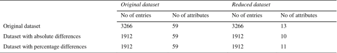
companies with their 2005-2007 yearly financial records (balance and income statement) from financial EDGAR database. Each instance has 59 financial attributes (indices used in financial analysis). This dataset was also transformed into differences between ratios using Step 4; both datasets with absolute differences and differences in percents were created. This step was applied in order to transform dataset into type of data usually used in financial analysis. Table 1 presents main characteristics of original and transformed datasets.

Table 1. Main characteristics of datasets used in experiments

Original dataset Reduced dataset

No of entries No of attributes No of entries No of attributes

Original dataset 3266 59 3266 13

Dataset with absolute differences 1912 59 1912 10 Dataset with percentage differences 1912 59 1912 11

To select the most important ratios feature selection was also applied for these datasets by using correlation-based feature subset selection algorithm with tabu search for search in attribute subsets. This step is also important as it gives an insight into what could be the most important ratios used to construct a risk evaluation model which could be applied in real process. The subsets of these turned out to be different; characteristics of obtained datasets are also presented in Table 1.

Table 2. Results of full dataset

Classifier Kernel function /SVM type Dataset with ratios Abs. difference dataset Perc. difference dataset

Training time No SV Accuracy Training time No SV Accuracy Training time No SV Accuracy

LibLINEAR L2-regularized L1-loss SVC 0,710 - 83,528 0,430 - 81,882 0,860 - 79,965

C-SVC RBF 0,610 570 79,155 0,510 524 82,753 0,510 494 82,753

SMO polynomial 0,844 - 82,449 1,562 - 82,927 0,719 - 82,753

SMO Pearson 13,407 898 83,061 3,297 1168 82,753 3,781 1217 82,753

Pegasos - 3,313 - 84,286 2,047 - 82,23 1,922 - 81,882

SGD - 3,812 - 83,265 2,234 - 83,275 2,172 - 82,753

mySVM RBF 3,812 N/A 82,959 1,328 N/A 82,927 1,203 N/A 83,972

CVM RBF 0,875 607 78,571 1,515 1043 82,753 2,172 1112 82,753

CVM Laplacian 1,094 783 78,571 0,906 1104 82,753 1,125 1175 82,753

CVM inverse distance 0,672 801 78,571 0,766 1125 82,753 0,969 1183 82,753

CVM inverse square distance 0,735 620 78,571 1,312 1033 82,753 1,844 1098 82,753

CVM-LS RBF 2,344 846 78,571 3,031 1106 82,753 4,891 1118 82,753

CVM-LS Laplacian 13,453 1600 78,571 9,781 1338 82,753 12,844 1338 82,753

CVM-LS inverse distance 13,437 1600 78,571 8,828 1338 82,753 8,781 1338 82,753

CVM-LS inverse square distance 2,453 942 78,571 2,828 1089 82,753 3,344 1096 82,753

BVM RBF 1,891 691 78,571 2,078 1066 82,753 2,734 1121 82,753

BVM Laplacian 0,750 728 78,571 0,781 982 82,753 1,218 1063 82,753

BVM inverse distance 0,672 743 78,571 0,688 992 82,753 1,031 1064 82,753

BVM inverse square distance 1,875 681 78,571 1,890 1026 82,753 2,360 1093 82,753

SVMLight RBF 22,48 1 78,570 14,80 1 82,93 15,61 1 82,23

Average: 80,006 82,736 82,605

For training, data was normalized and scaled to fit into interval [-1;+1]. Three risk classes were formed, as in original Altman model – “good”, “average” and “bad”. For change evaluation, three classes were also formed:

• 0 (or “decrease”) – if Altman-based evaluation shows a decrease in risk evaluation (thus the bankruptcy risk increases);

• 1 (or “stable”) – if this evaluation stays the same (risk also stays the same);

• 2 (or “increase”) – if there is an increase in discriminant evaluation (the possibility of bankruptcy decreases). It is important to note that financial ratios existing in original Altman mode1 which were used in evaluation were not used in order to avoid linear dependence between variables.

The experiment was run using several SVM implementations: original LibSVM 2.91 package by Chang and Lin, LibLINEAR 1.6 by Lin et. al., WEKA implementations of SMO, SGD and Pegasos, LibCVM 2.2 by Tsang et. al, RapidMiner’s mySVM implementation and multiclass version of SVMLight by Joachims. 70% of data was selected as training data and the remaining 30% - as testing data. Default parameters were used to train classifiers. For first part (three datasets with 59 attributes each) RBF kernel was selected experimentally for all nonlinear SVM classifiers, yet CVM, CVM-LS and BVM classifiers were also applied with Laplacian, inverse distance and inverse square distance functions as kernels.

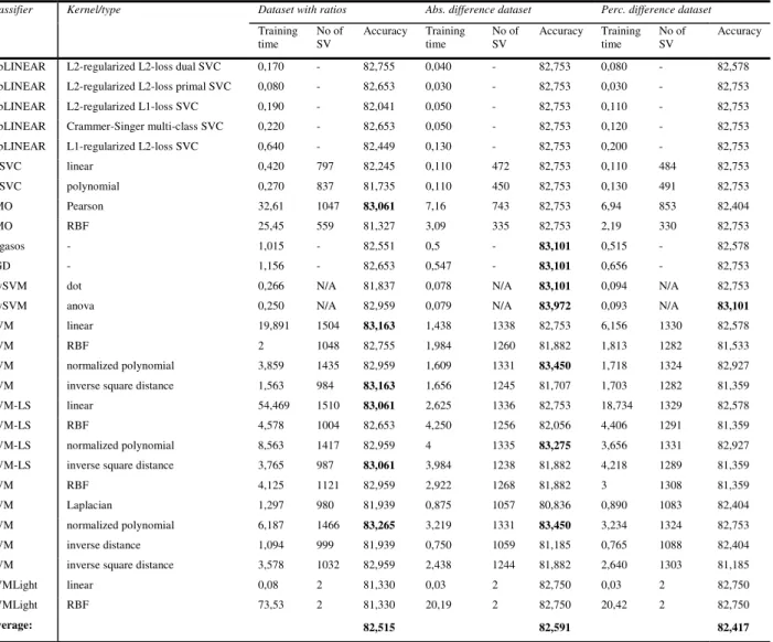
Table 3. Results of experiment with reduced data

Classifier Kernel/type Dataset with ratios Abs. difference dataset Perc. difference dataset

Training time No of SV Accuracy Training time No of SV Accuracy Training time No of SV Accuracy

LibLINEAR L2-regularized L2-loss dual SVC 0,170 - 82,755 0,040 - 82,753 0,080 - 82,578 LibLINEAR L2-regularized L2-loss primal SVC 0,080 - 82,653 0,030 - 82,753 0,030 - 82,753 LibLINEAR L2-regularized L1-loss SVC 0,190 - 82,041 0,050 - 82,753 0,110 - 82,753 LibLINEAR Crammer-Singer multi-class SVC 0,220 - 82,653 0,050 - 82,753 0,120 - 82,753 LibLINEAR L1-regularized L2-loss SVC 0,640 - 82,449 0,130 - 82,753 0,200 - 82,753

C-SVC linear 0,420 797 82,245 0,110 472 82,753 0,110 484 82,753 C-SVC polynomial 0,270 837 81,735 0,110 450 82,753 0,130 491 82,753 SMO Pearson 32,61 1047 83,061 7,16 743 82,753 6,94 853 82,404 SMO RBF 25,45 559 81,327 3,09 335 82,753 2,19 330 82,753 Pegasos - 1,015 - 82,551 0,5 - 83,101 0,515 - 82,578 SGD - 1,156 - 82,653 0,547 - 83,101 0,656 - 82,753

mySVM dot 0,266 N/A 81,837 0,078 N/A 83,101 0,094 N/A 82,753

mySVM anova 0,250 N/A 82,959 0,079 N/A 83,972 0,093 N/A 83,101

CVM linear 19,891 1504 83,163 1,438 1338 82,753 6,156 1330 82,578

CVM RBF 2 1048 82,755 1,984 1260 81,882 1,813 1282 81,533

CVM normalized polynomial 3,859 1435 82,959 1,609 1331 83,450 1,718 1324 82,927

CVM inverse square distance 1,563 984 83,163 1,656 1245 81,707 1,703 1282 81,359

CVM-LS linear 54,469 1510 83,061 2,625 1336 82,753 18,734 1329 82,578

CVM-LS RBF 4,578 1004 82,653 4,250 1256 82,056 4,406 1291 81,359

CVM-LS normalized polynomial 8,563 1417 82,959 4 1335 83,275 3,656 1331 82,927

CVM-LS inverse square distance 3,765 987 83,061 3,984 1238 81,882 4,218 1289 81,359

BVM RBF 4,125 1121 82,959 2,922 1268 81,882 3 1308 81,359

BVM Laplacian 1,297 980 81,939 0,875 1057 80,836 0,890 1083 82,404

BVM normalized polynomial 6,187 1466 83,265 3,219 1331 83,450 3,234 1324 82,753

BVM inverse distance 1,094 999 81,939 0,750 1059 81,185 0,765 1088 82,404

BVM inverse square distance 3,578 1032 82,959 2,438 1244 81,882 2,640 1303 81,185

SVMLight linear 0,08 2 81,330 0,03 2 82,750 0,03 2 82,750

SVMLight RBF 73,53 2 81,330 20,19 2 82,750 20,42 2 82,750

Average: 82,515 82,591 82,417

As some of the classifiers (such as SGD, Pegasos, mySVM) were implemented to solve only binary problems, “1-vs-1” method to use for transforming the multi-class problem into several 2-class ones was applied, thus training SVM classifiers as a set of binary classifiers. However, classifiers based on some implementations (such as mySVM) which are oriented to binary classification produced several sets of support vectors; in this case the

number of produced support vectors was marked as N/A (not available). Linear SVM classifiers (LIBLINEAR, SGD, Pegasos) produced a set of weights instead of a set of SV, thus the number of SV was not included in their cases. Linear SVM classifiers and nonlinear classifiers with linear, RBF and polynomial kernels were applied for reduced datasets. Table 2 shows the results obtained after performing the described procedure to original data, whereas Table 3 presents the results obtained with “reduced” datasets.

The test was run on a 2GHz Pentium Dual Core CPU PC with 3 GB of RAM. Metrics, presenting accuracy (classification accuracy), generated model complexity (no of support vectors) and training time, were chosen for evaluation; yet, it is important to mention that classifiers are written in different programming languages (SMO, Pegasos and mySVM are implemented in JAVA, others in C/C++), thus speed cannot be the main factor in evaluation.

3.5. Evaluation of results

The results show that feature selection performed an important part in construction process, as training time decreased from 4 to 10 times or more, yet accuracy was even better than performed with original data, which shows that the eliminated variables were not the most relevant. The results obtained while training original untransformed dataset varied; however, linear and gradient descent SVM classifiers, such as Pegasos, L2-regularized L1-loss SVC and SGD generated results with highest accuracy (84,286, 83,528 and 83,265 respectively), although RBF kernel selection with nonlinear SVM was also a good choice as it obtained better results than nonlinear classifiers with other kernels. The results, obtained after training data with differences, show that best results were obtained by mySVM based classifier, using RBF kernel; usage of linear classifiers SGD and Pegasos also resulted in results which are above 83%. Other results were similar and this shows that kernel function selection did not have much influence, especially in case of dataset with percentages where similar results were obtained with all classifiers. This is why most results obtained with transformations of original dataset were above average results of all classifiers.

However, CVM and BVM based classifiers outperformed others when performing classification procedure on reduced dataset; the choice of linear, inverse square distance and inverted polynomial kernels would be the best here although they are not fastest. Selection of linear kernel and linear classifiers resulted in good performance in terms of accuracy and training time in all three cases here as the results were above average results of tested classifiers. The results for the last two datasets (consisting of differences, together with applied feature selection), of almost all classifiers vary; CVM and BVM classifiers with normalized polynomial kernel function outperformed others, although they were not as fast as linear classifiers. Thus CVM and BVM classifiers are a good choice for further model development as they are trained fast enough (although not as fast as linear SVM classifiers) and produce high accuracy. However, they also produce the highest number of SVs (highest complexity); yet, the tests of their authors show, that the number of SV does not tend to grow less, compared to other SVM implementations (particularly LibSVM or SimpleSVM)[27].

4. Current limitations and future work

Experiment results showed that feature selection resulted even in better accuracy with which bankruptcy class can be predicted with accuracy ranging from 82 to 84%; however, efficiency of SVM classifiers much depends on parameter selection, thus obtained results can be improved by proper parameter selection, i.e., by using one of stochastic search or evolutionary techniques such as genetic algorithms or particle swarm optimization. Combination of SVM with these techniques is extensively researched and widely discussed in many papers. Another aspect especially important in this model application is dataset balance as classes are computed dynamically. SVM is one of the machine learning techniques which is sensitive to dataset imbalance as “majority” classes tend to outweigh “minority” classes by pushing classification boundaries over them. However, many techniques are applied to overcome this barrier: internally implemented class-weighting, cost-sensitive learning and evaluation [30][31], internal classifier enhancements [32][33], as well numerical sampling techniques, such as bootstrap [34], undersampling, oversampling and etc. Holte showed that minority random oversampling technique could be the best choice for SVM classifier [35]. Dataset balancing is crucially important in identification of bankrupt companies if they are represented by minority entries, as identification of bankrupt company might cost more to the creditor than the misidentification of it.

5. Conclusions

This article presents a empirical evaluation of SVM-based classifiers applied for credit risk evaluation task. Several classifiers, particularly linear LIBLINEAR, stochastic gradient based Pegasos and SGD, LibSVM C-SVC, mySVM, SMO, SVMLight, Core Vector Machines (CVM) and Ball Vector Machines (BVM), were applied for real-world dataset, together with widely applied discriminant Altman technique as a basis for output formation. The methodology presented in this article could serve as a alternative tool for risk analysis in case when there are no actual bankruptcy classes or obtaining them might be a too complicated or expensive. The dataset was evaluated in three ways: as original (unchanged) dataset and transformed into differences expressed as absolute and percentage values respectively. A feature selection algorithm based on correlation-based feature subset selection was also applied in order to reduce the dimensionality of the dataset thus leaving only the most relevant ratios, and the classifiers were rerun on datasets based on the same principle as described above.

This research also showed that linear SVM classifiers, together with gradient descend based SVM classifiers and Core Vector Machines algorithms, can be a good choice or alternative for implementation of SVM-based credit risk evaluation model.

References

1. E. I. Altman, Predicting financial distress of companies: revisiting the Z-score and ZETA models. working paper, Stern School of Business, New York University, New York (2000)

2. M. Zmijewski, Methodological Issues Related to the Estimation of Financial Distress Prediction Models, Journal of Accounting Research (1984), Vol. 22, pp.59–82

3. E. G. Sands, G. L.V. Springate, Predicting Business Failures. CGA Magazine (1983), pp. 24-27

4. E. Merkevicius, G. Garsva, S. Girdzijauskas, A hybrid SOM-Altman model for bankruptcy prediction, Lecture Notes in Computer Science (2006), Vol. 3994, pp. 364-371.

5. E. Merkevicius, G. Garsva, R. Simutis, Neuro-discriminate Model for the Forecasting of Changes of Companies Financial Standings on the Basis of Self-organizing Maps, Lecture Notes In Computer Science, Berlin, Heidelberg: Springer-Verlag (2007), pp. 439-446. 6. W. Chen, J. Shih, A study of Taiwan’s issuer credit rating systems using support vector machines, Expert Systems with Applications

(2006), Vol. 30, pp.427-435.

7. Z. Huang, H. Chen, C.J. Hsu, W.H. Chen, S. Wu, Credit rating analysis with support vector machines and neural networks: a market comparative study, Decision Support Systems (2004), Vol. 37, pp. 543–558.

8. K.Kim, Financial time series forecasting using support vector machines. Neurocomputing (2003), Vol. 55, pp.307–320

9. B. Ribeiro, A. Vieira, J. Duarte, C. Silva, J. Carvalho das Neves, S. Mukkamala, A. H. Sung, Bankruptcy Analysis for Credit Risk using Manifold Learning, Advances in Neuro-Information Processing, Lecture Notes in Computer Science (2009), Vol. 5506., pp. 723-730 10. W.Chong, G. Yingjian, W. Dong, Study on Capital Risk Assessment Model of Real Estate Enterprises Based on Support Vector

Machines and Fuzzy Integral, Control and Decision Conference (2008), pp. 2317-2320.

11. T. Van Gestel, B. Baesens, J. A.K. Suykens, D. Van den Poel, D.-E. Baestaens et. al. Bayesian kernel based classification for financial distress detection. European Journal of Operational Research (2006), Vol. 172(3), pp. 979-1003.

12. H. Ahn, K. Lee, K. Kim, Global Optimization of Support Vector Machines Using Genetic Algorithms for Bankruptcy. Lecture Notes in Computer Science, Springer (2006), Vol. 4234(5), pp. 420-9.

13. P.Y. Hao, M.S. Lin, L.B. Tsai, A New Support Vector Machine with Fuzzy Hyper-Plane and Its Application to Evaluate Credit Risk, Proceedings of Eighth International Conference on Intelligent Systems Design and Applications (2008), pp. 83-8.

14. B. Wang, Y. Liu, Y. Hao, S. Liu, Defaults Assessment of Mortgage Loan with Rough Set and SVM, Proceedings of the International Conference on Computational Intelligence and Security (2007), pp. 981–5.

15. J. Zhou, A. Zhang, T. Bai, Client Classification on Credit Risk Using Rough Set Theory and ACO-Based Support Vector Machine, 4th International Conference on Wireless Communications, Networking and Mobile Computing (2008), pp.1-4

16. J.M.Y. Xuchuan, “Construction and Application of PSO-SVM Model for Personal Credit Scoring, Chinese Journal of Management (2008), Vol. 4, pp. 158-161.

17. P. Danenas,G. Garsva, Support Vector Machines and their Application In Credit Risk Evaluation Process, Transformations in Business & Economics (2009), Vol. 8, No. 3 (18), pp. 46-58

Berlin, Springer, Vol. 57, Part 1, pp. 7-12

19. K. K. Lai, L. Zhou, S. Wang, Credit Risk Evaluation with Least Square Support Vector Machine, Lecture Notes in Computer Science (2006), Vol. 4062, pp. 490-5

20. T. Van Gestel, B. Baesens, J. Suykens, M. Espinoza, D. Baestaens, J. Vanthienen et al., Bankruptcy prediction with least squares support vector machine classifiers, Proceedings on IEEE International Conference on Computational Intelligence for Financial Engineering (2003). pp. 1-8.

21. C. Chang, C. Lin, LIBSVM: a Library for Support Vector Machines (2001). 22. V. Vapnik, The Nature of Statistical Learning Theory, Springer-Verlag (2000).

23. R. Fan, K. Chang, K., Hsieh, C., Wang, X., Lin, C., LIBLINEAR: A library for large linear classification, The Journal of Machine Learning Research(2008), Vol. 9, pp.1871–4.

24. J. Platt, Sequential minimal optimization: A fast algorithm for training support vector machines, Advances in Kernel Methods-Support Vector Learning (1999), 208, pp.98-112.

25. S. Shalev-Shwartz, Y. Singer, N. Srebro, Pegasos: Primal Estimated sub-GrAdient SOlver for SVM, 24th International Conference on Machine Learning (2007), pp. 807-814.

26. S. Rüping, mySVM-Manual, University of Dortmund, Lehrstuhl Informatik 8, http://www-ai.cs.uni-dortmund.de/SOFTWARE/MYSVM (2000)

27. W. Tsang, J. T. Kwok, P. M. Cheung, Core vector machines: Fast SVM training on very large data sets, Journal of Machine Learning Research (2005), Vol. 6, pp.363-392.

28. I. W. Tsang, A. Kocsor, J. T. Kwok. Simpler core vector machines with enclosing balls. Proceedings of the Twenty-Fourth International Conference on Machine Learning, Corvallis, Oregon, USA (2007), pp.911-8.

29. T. Joachims, Making large-Scale SVM Learning Practical. Advances in Kernel Methods - Support Vector Learning, B. Schölkopf and C. Burges and A. Smola (ed.), MIT-Press, 1999

30. Ch. Elkan, The Foundations of Cost-Sensitive Learning, International Joint Conference on Artificial Intelligence (2001), Vol. 17(1), pp. 973-8.

31. N. Thai-Nghe, Z. Gantner, L. Schmidt-Thieme, Cost-sensitive learning methods for imbalanced data. The 2010 International Joint Conference on Neural Networks (IJCNN) (2010), pp. 1-8.

32. S. Lessmann, Solving imbalanced classification problems with support vector machines, International Conference on Artificial Intel- ligence (2004), pp. 214–220.

33. Y.F. Li, J.T. Kwok, Z.H. Zhou, Cost-Sensitive Semi-Supervised Support Vector Machine, Artificial Intelligence (2010), pp. 500-5. 34. D. D. Margineantu, Th. G. Dietterich, Bootstrap Methods for the Cost-Sensitive Evaluation of Classifiers, Proceedings of the

Seventeenth International Conference on Machine Learning (2000), pp. 583-590.

35. J. Van Hulse, T.M. Khoshgoftaar, A. Napolitano, Experimental perspectives on learning from imbalanced data, Proceedings of the 24th international conference on Machine learning - ICML ’07 (2007), pp. 935-942.