DIPARTIMENTO DI INFORMATICA, SISTEMISTICA E COMUNICAZIONE DOTTORATO DI RICERCA IN INFORMATICA - CICLO XXV
Ph.D. Thesis
Algorithms for Next Generation
Sequencing Data Analysis
Author:
Stefano
Beretta
Advisors:
Prof.ssa Paola
Bonizzoni
Prof. Gianluca
Della Vedova
First and foremost, I want to thank my parents for their love and support throughout my life. Thank you both for giving me everything. This thesis would certainly not have existed without them.
I would like to thank my two advisors, Prof. Paola Bonizzoni and Prof. Gianluca Della Vedova for their guidance during my Ph.D.
I am extremely grateful to Yuri Pirola, Raffaella Rizzi and Riccardo Dondi for their continuous encouragement and for the useful discussions. Their contribution has been fundamental.
A special thank goes to Mauro, my colleague and my friend. I have spent wonderful moments with him and I could not have a better mate.
My thanks go to all my office mates, Luca, Enrico and Carlo, and to my other Ph.D. colleagues, Lorenza and Luca, with whom I shared good and bad moments during these three years.
I wish to acknowledge all the people I met during the Ph.D., and in particular to the patience and understanding shown by Laura, Ilaria and Gaia to me. It must not have been easy to bear with me. I would also like to offer my special thanks to Silvia and Elena, for their wonderful encouragement.
I am grateful to all my friends, especially Mauro and Stefano. I have known them for a long time and spending my spare time with them is always wonderful.
Me gustar´ıa agradecer al Prof. Gabriel Valiente por dirigirme durante mi estancia en laUniversitat Polit`ecnica de Catalunya y a Daniel Alonso-Alemany por las discusiones fruct´ıferas y por toda su ayuda. Trabajar con ellos ha sido un verdadero placer.
Tambi´en quiero dar las gracias a Jorge, Alessandra, Ramon, Javier, Nikita, Eva, Albert y todos los otros compa˜neros del despacho.
Acknowledgements iii
List of Figures vii
List of Tables x
1 Introduction 1
2 Background 6
2.1 DNA and RNA . . . 6
2.2 Gene and Alternative Splicing . . . 7
2.3 Sequencing . . . 10
2.3.1 Sanger Technique. . . 10
2.3.2 Next Generation Sequencing . . . 11
2.4 Data . . . 21
2.4.1 RNA-Seq . . . 24
2.5 Definitions. . . 25
2.5.1 Strings. . . 25
2.5.2 Graphs and Trees. . . 26
3 Reconstructing Isoform Graphs from RNA-Seq data 31 3.1 Introduction. . . 32
3.1.1 Transcriptome Reconstruction . . . 34
3.1.2 Splicing Graph . . . 39
3.2 The Isoform Graph and the SGR Problem . . . 41
3.3 Unique solutions to SGR. . . 45
3.4 Methods . . . 46
3.4.1 Isomorphism between predicted and true isoform graph . . . 50
3.4.2 Low coverage, errors and SNP detection . . . 51
3.4.3 Repeated sequences: stability of graphGR. . . 52
3.5 Experimental Results. . . 53
3.6 Conclusions and Future Work . . . 60
4 Taxonomic Assignment to Multiple Trees in Metagenomics 63 4.1 Introduction to Metagenomics. . . 65
4.1.1 Taxonomic Alignment . . . 68
4.1.2 Taxonomic Assignment with TANGO . . . 69
4.2 Taxonomy Analysis . . . 72
4.2.1 16S Databases . . . 73
4.2.2 Tree Analysis . . . 74
4.2.3 Inferring Trees from Lineages . . . 76
4.3 Minimum Penalty Score Calculation . . . 81
4.3.1 An Asymptotically Optimal Algorithm. . . 82
4.4 TANGO Improvement . . . 86
4.4.1 New Data Structures. . . 86
4.4.2 Optimal Algorithm Implementation . . . 89
4.4.3 Input Mapping . . . 91
4.5 Conclusions and Future Work . . . 92
A Additional Data 96
2.1 The central dogma of molecular biology. The DNA codes for the produc-tion of messenger RNA during transcripproduc-tion, which is then translated to proteins. . . 7
2.2 Basic types of alternative splicing events. . . 9
2.3 Sanger sequencing process. Figure 2.3(a) illustrates the products of the polymerase reaction, taking place in the ddCTP tube. The polymerase ex-tends the labeled primer, randomly incorporating either a normal dCTP base or a modified ddCTP base. At every position where a ddCTP is inserted, the polymerization terminates; the final result is a population of fragments. The length of each fragment represents the relative dis-tance from the modified base to the primer. Figure 2.3(b) shows the electrophoretic separation of the products of each of the four reaction tubes (ddG, ddA, ddT, and ddC), run in individual lines. The bands on the gel represent the respective fragments shown to the right. The complement of the original template (read from bottom to top) is given on the left margin of the sequencing gel. . . 12
2.4 Roche 454 sequencing. In the library construction, the DNA is frag-mented and ligated to adapter oligonucleotides, and then the fragments are clonally amplified by emulsion PCR. The beads are then loaded into picotiter-plate wells, where iterative pyrosequencing process is performed. 14
2.5 Illumina sequencing 1/3. The DNA sample is fragmented and the adapters are bound to the ends (Figure 2.5(a)); the obtained single-strained frag-ments are attached to the flow cell surface (Figure 2.5(b)) and then they are “bridged” (Figure 2.5(c)). . . 16
2.6 Illumina sequencing 2/3. The fragments become double-strained (Fig-ure 2.6(a)) and then they are denat(Fig-ured. This process leaves anchored single-strained fragments (Figure 2.6(b)). After a complete amplification, millions of clusters are formed on the flow cell surface (Figure 2.6(c)). . . 16
2.7 Illumina sequencing 3/3. The clusters are washed, leaving only the for-ward strands and, to initiate the sequencing process, primer, polymerase and a 4 colored terminators are added. The primers are bound to the primers of the strand and, after that, the first terminator is incorpo-rated (Figure 2.7(a)). By iterating the incorporation process, all the sequence nucleotides are added and the laser activates the fluorescence (Figure 2.7(b)). During the incorporation a computer reads the image and determines the sequence of bases (Figure 2.7(c)). . . 17
2.8 Sequencing by ligation. In (1) the primer is annealed to the adaptor and the first two bases of the probe are bound to the first two bases of the sequence. The fluorescence signal is read (2) and the last bases of the probe are cleaved, so that the new phosphate group is created (3). This ligation process is repeated for seven cycles (4), in order to extend the primer. Finally, this latter primer is melted off and a new one is annealed (5). The previous steps are repeated for all the new primers, with different offsets (6). . . 19
2.9 Summary of the sequencing by ligation process showing, for each base of the read sequence, the positions of the interrogations (2 for each position). 19
2.10 Examples of graphs. Both the graphs have 5 nodes and 7 edges, but in Figure 2.10(a) the edges are unordered (i.e. (u, v) = (v, u)) and they are represented as simple lines. Instead in Figure 2.10(b) the edges are ordered (i.e. (u, v)6= (v, u)) and they are represented as arrows indicating the direction. . . 26
2.11 Example ofDe Bruijn graph on the binary alphabet, with k= 4. Nodes represent all the possible substrings of length k−1 and there is an edge between two nodes if there is a k-mer that has the first (k−1)-mer as prefix and the second (k−1)-mer as suffix. The k-mer is obtained by the fusion of the (k−1)-mers at the two ends. In this example edges are labeled by the symbols that must be concatenated to the first (k−1)-mer, to obtain thek-mer. . . 28
2.12 Example of rooted tree. The noder is the root of the tree, the nodes n3,
n4, n5,n7, n9,n10 and n11 are the leaves and n1,n2, n6 and n8 are the
internal nodes. As an example,n6 is the parent ofn8and n2 is one of the
children of n1 (the other one isn5).. . . 29
2.13 Example of tree traversals. Given the tree, this example shows the order in which the nodes are visited, for each of the three types of traversal. . . 30
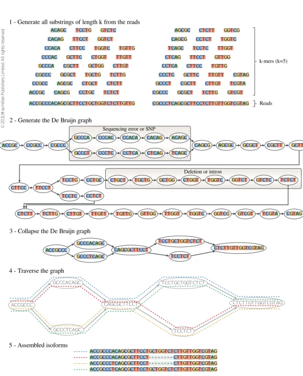
3.1 Genome Independent assembly. Reads are split into k-mers (1) and the
De Bruijn graph is built, with the possibility of having sequencing errors or SNPs and also deletions or introns, that generate different branches (2). The graph is then contracted by collapsing all its linear paths (3). The contracted graph is traversed (4) and each isoform is assembled from an identified path (5). . . 38
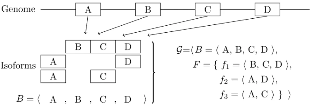
3.2 Example of expressed gene. Given a gene in which its isoforms are com-posed of blocks (that for simplicity are associated to exons: A,B,C and
D) extracted from the genome, we represent the sequence B of blocks based on the (genomic) position. The expressed geneG =hB, Fi is con-structed from the block sequence B and its isoform composition. . . 42
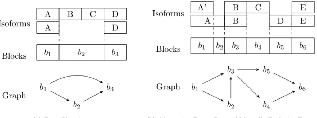
3.3 Examples of Isoform Graphs. These two examples show the isoform com-position of a gene (1) with the corresponding block sequence (2) and their isoform graphs (3). Capital letters correspond to exons. In (a) is repre-sented a skipping of the two consecutive exons B and C of the second isoform w.r.t. the first one. In (b) is represented an alternative donor site variant between exons AandA0 and two mutually exclusive exonsC and
D. Notice that, in this figure, the isoforms represented are classical. . . . 43
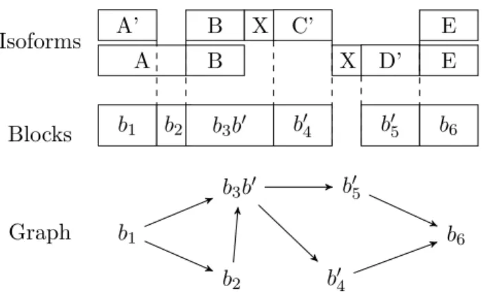
3.4 Alternative splicing graph compatible with the reads of the expressed gene of Figure 3.3(b) . . . 44
3.5 Example of read classification. The example shows two transcripts, where the first one is composed of 3 blocks (A, B and C) and the second one of 2 blocks (A and C). Moreover, reads coming from those blocks are partitioned into unspliced (white rectangles) and spliced (gray rectangles). Notice that the two reads sharing the same suffix of blockA(of lengthk) and those two sharing the same prefix of blockC (of lengthk) are labeled withsuf(A, k) and pre(C, k), respectively. . . 47
3.6 Sn and PPV values at vertex level in the first 3.6(a) and in the sec-ond 3.6(b) experiments. Each point represents a gene. . . 57
3.7 Sn and PPV values at arc level in the first 3.7(a) and in the second 3.7(b) experiments. Each point represents a gene. . . 58
3.8 Gene POGZ. The correct isoform graph (on the left) and the predicted isoform graph (on the right) predicted in the third experiment. Number in the nodes represent the lengths of the blocks. The difference between the two graphs consists of the gray vertex that is missing in the predicted graph. . . 59
4.1 Example of taxonomic tree. The example shows a rooted tree with max-imum depth 8 (7 taxonomic ranks plus the Root), underling a subset of nodes and their associated taxonomic ranks. . . 67
4.2 Leaf set partition used for the Penalty Score calculation in TANGO. In this example, given a read Ri ∈R the matches are represented as circled
leaves, i.e. Mi = {S1, S5, S6, S7}. The leaves of Ti, which is the subtree
rooted at the LCA of Mi, can be partitioned into 4 disjointed subsets
(T Pi,j,F Pi,j,T Ni,j and F Ni,j) for each node j inTi. Ti,j represents the
subtree ofTi induced by the choice of node j as representative of Mi.. . . 72
4.3 Example of tree with its representation in Newick format. . . 75
4.4 Example of “binarization process”. On the left there is an example of tree in which a noder has 4 children (named n1,n2,n3 andn4). On the
right there is the same tree after the binarization, in which the circled node are the ones added in the process. . . 76
4.5 An example of rooted tree T is shown in 4.5(a), where the circled leaves are the ones in the set S, i.e.S ={3,4,9,11}. In 4.5(b) the skeleton tree obtained from Definition 4.2, starting from the tree T and the subset of leaves S. . . 82
4.6 Example of tree and the corresponding data structure obtain by taking the nodes as ordered from left to right (according to the picture). In particular, for each node we use three pointers: parent, f irst-child and
next-sibling. Notice the following special cases: the Root node (which has itself as parent), the leaves (which do not have a first child) and the last siblings (which do not have the next sibling). . . 87
2.1 Roche/454 Life Sciences NGS instruments.. . . 15
2.2 Illumina/Solexa NGS instruments. . . 17
2.3 Life Technologies/SOLiD NGS instruments. . . 20
2.4 Error rate comparison of different sequencing platforms. . . 22
2.5 Quality score and base calling accuracy. . . 22
4.1 List of the main databases for 16S ribosomal RNA (rRNA) and the num-ber of Bacteria and Archaea (high-quality) sequences present in the cur-rent version of the database.. . . 73
4.2 Statistics on the taxonomic trees. In the specific, the second column reports the type of the tree which can be n-ary or binary; the third and fourth columns report the number of leaves and total nodes, respectively; the last column reports the maximum depth of the tree. . . 77
4.3 Statistics on the reconstructed RDP taxonomy. In the specific, for each depth of the tree, the number of nodes (resp. leaves) is reported. . . 78
A.1 Details of the first experiment of Section 3.5. . . 96
A.2 Details of the second experiment of Section 3.5. . . 100
Introduction
Due to the continuously growing amount of produced data, methods in computer science are becoming more and more important in biological studies. More specifically, the advent of Next-Generation Sequencing (NGS) techniques has opened new challenges and perspectives that were not even thinkable some years ago. One of the key points of these new methods is that they are able to produce a huge quantity of data at much lower costs, with respect to the previous sequencing techniques. Moreover, the growth rate of these data is higher than the one of semiconductors, meaning that approaches based on Moore’s law do not work. This also means that algorithms and programs that were used in the past are no longer applicable in this new “context” and so new solutions must be found. This is mainly due to two main reasons. On one hand, data are of different nature. In fact, the produced sequences are much shorter than the ones of the classical methods. On the other hand, also the volume of data is changed, as the new methods can produce millions or billions of sequences, that is orders of magnitude more than before. Hence, efficient procedures are required to process NGS data. Moreover, new approaches are necessary to face the continuously emerging computational problems, that are fundamental to take advantage of the produced data. Two of the fields in bioinformatics that are most influenced, by the introduction of the Next-Generation Sequencing methods, are transcriptomics and metagenomics. In this thesis we address two central problems of these latter fields.
The central goal in transcriptome analysis is the identification and quantification of all full-length transcripts (or isoforms) of genes, produced by alternative splicing. This mechanism has an important role in the regulation of the protein expressions that in-fluences several cellular and developmental processes. Moreover, recent studies point out that alternative splicing may also play a crucial role in the differentiation of stem cells, thus opening a new perspective in transcriptome analysis [1]. Understanding such
a mechanism can lead to new discoveries in many fields. Therefore, a lot of effort has been invested in the study of methods for alternative splicing analysis and full-length transcript prediction, which, however, operate on data produced by the old Sanger tech-nology. On the other hand, NGS technologies have opened new possibilities in the study of the alternative splicing, since data from different individuals and cells are available for large scale analysis. With the specific goal of analyzing NGS data, some computational methods for assembling full-length transcripts or predicting splice sites from such data have been recently proposed. However, these tools by alone are not able to provide an overview of alternative splicing events of a specific set of genes. In particular, a challeng-ing task is the comparison of transcripts derived from NGS data to predict AS variants and to summarize the data into a biological meaningful set of AS events. Another issue involves the prediction of AS events from NGS data without a specific reference genome, as the currently available tools can perform this task with limited accuracy, even with the presence of a reference.
In this thesis, to tackle the previously mentioned issues:
1. we face the problem of providing a representation of the alternative splicing vari-ants, in absence of the reference genome, by using the data coming from NGS techniques;
2. we provide an efficient procedure to construct such a representation of all the alternative splicing events.
The solution we propose for the first problem is the definition of theisoform graph, which is a graph representation that summarize all the full-length transcripts of a gene. We investigate the conditions under which it is possible to construct such a graph, by using only RNA-Seq reads, which are the sequences obtained when sequencing a transcript with NGS methods. These conditions guarantee the possibility to obtain the correct graph from the NGS data. We analyze each condition in detail, in order to explore the possibility of reconstructing the isoform graph in absence of a reference genome.
For the second problem we propose a solution to construct the isoform graph, also when the necessary conditions, for its complete reconstruction, are not satisfied. In the latter case the obtained graph is an approximation of the correct one. The algorithm we propose is a three-step procedure in which the reads are first partitioned into two subsets and then assembled to create the graph. We also provide an experimental validation of this approach, which is based on an efficient implementation of the algorithm, that uses the RNA-Seq reads coming from one or more genes. More precisely, in order to verify its accuracy and its stability, we have performed different tests that reflect
different conditions of the input set. We show the scalability of our implementation to huge amount of data. Limiting computational (time and space) resources used by our algorithm is a main aim of ours, when compared to other tools of transcriptome analysis. Our algorithmic approach works in time that is linear in the number of reads, with space requirements bounded by the size of the hash tables used to memorize the sequences. Finally, our computational approach for representing alternative splicing variants is different from current methods of transcriptome analysis that focus on using RNA-Seq data for reconstructing the set of transcripts of a gene and estimating their abundance. More specifically, we aim to summarize genome-wide RNA-Seq data into graphs, each representing an expressed gene and the alternative splicing events occurring in the specific processed sample. On the contrary, current tools do not give a concise result, such as a structure for each gene, nor they provide a easy-to-understand list of alternative splicing events for a gene.
Part of this work has been presented in the following international venues:
• S. Beretta, P. Bonizzoni, G. Della Vedova, R. Rizzi, Reconstructing Isoform Graphs from RNA-Seq data., 2012, IEEE International Conference on Bioinfor-matics and Biomedicine (BIBM), 2012, Philadelphia PA, USA [2]
• Y. Pirola, R. Rizzi,S. Beretta, E. Picardi, G. Pesole, G. Della Vedova, P. Boniz-zoni,PIntronNext: a fast method for detecting the gene structure due to alternative splicing via ESTs, mRNAs, and RNA-Seq data., EURASNET Symposium on Reg-ulation of Gene Expression through RNA Splicing, 2012, Trieste, Italy
• S. Beretta, P. Bonizzoni, G. Della Vedova, R. Rizzi, Alternative Splicing from RNA-seq Data without the Genome., ISMB/ECCB - 8th Special Interest Group meeting on Alternative Splicing (AS-SIG), 2011, Vienna, Austria
• S. Beretta, P. Bonizzoni, G. Della Vedova, R. Rizzi,Identification of Alternative Splicing variants from RNA-seq Data., Next Generation Sequencing Workshop, 2011, Bari, Italy
The second part of this thesis is focused on a fundamental problem in metagenomics. The aim of this continuously growing field of research is the study of uncultured organisms to understand the true diversity of microbes, their functions, cooperation and evolution, in environments such as soil, water, ancient remains of animals, or the digestive system of animals and humans. With the advent of NGS technologies, which do not require cloning or PCR amplification, there has been an increase in the number of metagenomic projects. As anticipated, the use of NGS methods creates new problems and challenges in bioinformatics, which has to handle and analyze these datasets in an efficient and
useful way. A better understanding of the microbial world is one of the main goals of metagenomic studies and, in order to accomplish this challenge, the comparison among multiple datasets is a required task. Despite the improvement of various techniques, there is still a need for new computational approaches and algorithmic methods to find a solution to emerging problems related to NGS data analysis. One of these problems is the assignment of reads to a reference taxonomy. This task is crucial in identifying the species present in a sample and also to classify them. More specifically, starting from a set of NGS reads coming from a metagenomic sample, the objective is to assign them to a reference taxonomy, in order to understand the composition of the sample. In order to solve this problem, a commonly adopted technique is the alignment of reads to the taxonomy, followed by the correct assignment of ambiguous reads (i.e. the ones that have multiple valid matches) in the same taxonomy. This latter procedure is usually based on computing the Lowest Common Ancestor (LCA) of all the alignments of the read.
In the thesis we address some challenging open questions on the problem of assigning reads to a taxonomy, mainly:
1. having a fast and at the same time accurate procedure to process reads and assign them to the tree;
2. making possible the use of taxonomy that differ in the ranking of species.
The two above mentioned tasks are accomplished in this thesis by designing novel pro-cedures in the TANGO method. TANGO is an example of software that bases the assignment on the calculation of a penalty score function for each of the candidate nodes of the taxonomy. In particular, we improve the time efficiency and accuracy of TANGO by realizing an fast procedure for the computation of the minimum penalty score value of the candidate nodes, also supported by a more efficient implementation of the software. To do this, we take advantage of an algorithm for inferring the so called skeleton tree, given a tree and a subset of its leaves. We prove that it is possible to compute the penalty score in an optimal way by using the previously mentioned tree, and we provide an algorithmic procedure to accomplish this task. The latter method is implemented by using a simple data structure to represent the tree, which contributes to the improvement of performance of the overall method. The second main issue men-tioned before has been addresses by developing a method to contract the taxonomic trees keeping only specific ranks, in order to facilitate the comparison among different taxonomies. Our contributions provide an improvement to the problem of assigning the reads to a reference taxonomy, which is a basic step in a metagenomic analysis.
• D. Alonso-Alemany, A. Barre,S. Beretta, P. Bonizzoni, M. Nikolski, G. Valiente, Further Steps in TANGO: Improved Taxonomic Assignment in Metagenomics., 2012, (Submitted)
In the rest of this thesis all the results mentioned above are explained in detail. In Chapter 2 the biological notions, necessary for the understanding of the following descriptions, are introduced. In addition to this, the basic algorithmic concepts and no-tations are formalized, providing a complete background. Chapter 3starts with a brief introduction and describes the current approaches for the reconstruction of transcripts, from NGS data. Then the concept of isoform graph is explained and the necessary and sufficient conditions to construct such a graph, are provided. An algorithm for the computation of the isoform graph is given, with also a particular attention on its implementation. After that, an experimental validation, aimed to verify the accuracy of the predictions and also the stability of this method, is described. Finally, some conclusions and future developments of this approach are proposed. Chapter 4 re-ports the work in metagenomics, performed during my period abroad at theAlgorithms, Bioinformatics, Complexity and Formal Methods Research Group of the Technical Uni-versity of Catalonia in Barcelona, Spain, in collaboration with Daniel Alonso-Alemany, under the supervision of Prof. Gabriel Valiente. More specifically, after an introduc-tion to metagenomics, the problem of the taxonomic assignment is described, with a particular attention on the solution provided by the TANGO software. After that, we describe the proposed method to contract the main different available taxonomies. We also provide a description of the new data structures used to represent trees. The focus is then moved to the minimum penalty score calculation, and in particular, to the proof of this latter problem that involves the skeleton tree. Finally, all the improvements of the TANGO software are described and the chapter is concluded by underlining some possible developments of this work.
Background
In this chapter basic notions concerning the biological and algorithmic background are given. After the introduction of fundamental biological concepts, the attention is focused on the sequencing process by describing classical and new techniques. In particular, the Next-Generation Sequencing platforms are shown, discussing the methods they adopt. The produced data are then analyzed and the specific case of RNA-Seq is explained. Finally some algorithmic concepts and formal notations used in the rest of the thesis are introduced (for a more detailed explanation see [3]).
2.1
DNA and RNA
The deoxyribonucleic acid (DNA) molecule is the carrier of the genetic information in our cells. In fact all the information it contains are passed from organisms to their offspring during the process of reproduction. More specifically, each DNA molecule consists of the four nucleotides Adenine (A), Cytosine (C), Guanine (G), and Thymine (T), with backbones made of sugars and phosphate groups joined by ester bonds. It is organized as a double-helix and the two strands of the DNA molecule are complementary to each other. The base-pairing is fixed: A is always complementary to T, and G is always complementary to C. This double-helix model was proposed in 1953 by James Watson, an American scientist, and Francis Crick, a British researcher, and it has not been changed much since then. This discovery was made by studying the X-ray diffraction patterns, and this allowed to the two scientists to build models and to figure out the double-helix structure of DNA, a structure that enables it to carry biological information from one generation to the following.
Figure 2.1: The central dogma of molecular biology. The DNA codes for the produc-tion of messenger RNA during transcripproduc-tion, which is then translated to proteins.
The complete genome is composed of chromosomes which are a set of different DNA molecules. Eukaryotes, i.e. organisms that have cells with a structure made by mem-branes, store the chromosomes in the nuclei of their cells. For example, in humans, the genome has a total of more than 3 billion of nucleotides that are organized in 23 chromosomes, each of which appears in two copies in each cell. An important functional unit in a chromosome is the gene, which is described by the so calledcentral dogma of molecular biology.
The central dogma in molecular biology (shown in Figure 2.1) says that portions of DNA, called gene regions, are transcribed into ribonucleic acid (RNA), which is then translated into proteins. The RNA molecules differ from the DNA ones because they are often single strained and the Thymine (T) nucleotide is replaced by Uracil (U). In addition to this, the half-life of RNA molecules is shorter than that of DNA molecules. As mentioned before, RNA has a central role in protein synthesis, in fact a particular type of RNA, called messenger RNA, carries information from DNA to structures called ribosomes. These ribosomes, that are made from proteins and ribosomal RNAs, can read messenger RNAs and translate the information they carry into proteins. There are many types of RNAs with other roles and functions, in particular they can regulate the expression of some genes, and they are also present in the genomes of most viruses.
2.2
Gene and Alternative Splicing
From a molecular point of view, a gene is commonly defined as the entire nucleic acid sequence that is necessary for the synthesis of a functional polypeptide. According to this definition, in a gene there are not only the nucleotides that encode the amino acid
sequence of a protein (usually referred to as thecoding region), but there are also all the DNA sequences required for the synthesis of a particular RNA transcripts. The concept of gene has evolved and has become more complex since it was first proposed. There are various definitions of this term, but all the initial descriptions were focused on the ability to determine a particular characteristic of an organism and also the heritability of this characteristic. A modern definition of a gene is “a locatable region of genomic sequence, corresponding to a unit of inheritance, which is associated with regulatory regions, transcribed regions, and or other functional sequence regions” [4,5].
On the other side, the computational biology community has adopted a “definition” of gene as a formal language to describe the gene structure as a grammar, by using a precise syntax of upstream regulation, exon, and introns. More specifically, a gene is composed ofexons andintrons. The formers, which are usually referred as coding parts, are the essential parts of the messenger RNA (mRNA), that is the template sequence for the protein, whereas introns, which are usually referred as non-coding parts, mostly have a regulatory role. Following the central dogma, the complete gene region is first transcribed into a precursor mRNA (pre-mRNA) molecule that consists of exons and introns. Transcription is the first stage of the expression of genes into proteins.
During thetranscription process, some proteins, called transcription factors, bind in or near the promoter region that resides directly upstream of the gene. These proteins have the controlling role of the transcription. At this point, thesplicingprocess is initiated by RNA binding proteins, called splicing factors, and the intron sequences of the pre-mRNA are removed. This is typical in eukaryotes, in which the messenger RNA is subject to this process, in order have the correct production of proteins through translation. The recognition of intron-exon boundaries is facilitated through the detection of short sequences called splice sites.
At the end of the transcription, a process, called polyadenylation, is involved. Polyadeny-lation consists in the addition of a poly-A tail, which is a series of Adenine nucleotides, to a RNA molecule. The process of polyadenylation is initiated by the binding of pro-teins to the polyadenylation site of an exon in the pre-mRNA. After the splicing and the polyadenylation of the pre-mRNA, the final mRNA is obtained. The poly-A tail added in the polyadenylation process is important for the transport of the mRNA to the cell cytoplasm and also for the control of the half-life of the mRNA.
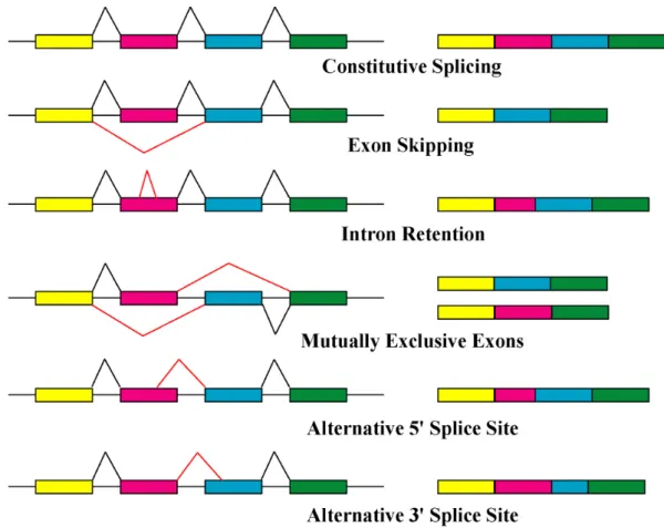
By varying the exon composition of the same messenger RNA, the splicing process can produce a set of unique proteins. This process is called alternative splicing (AS) and is the mechanism by which a single pre-mRNA can produce different mRNA variants, by extending, shortening, skipping, or including exon, or retaining intron sequences. The most recent studies indicate that alternative splicing is a major mechanism generating
Figure 2.2: Basic types of alternative splicing events.
functional diversity in humans and vertebrates, as at least 90% of human genes exhibit splicing variants.
In a typical mRNA (which is composed of several exons), there are different ways in which the splicing pattern can be altered (see Figure 2.2). Most exons are constitutive and they are always spliced or included in the final mRNA. A regulated exon that is sometimes included and sometimes excluded from the mRNA is called askipped exon(or cassette exon). In certain cases, multiple cassette exons aremutually exclusive, produc-ing mRNAs that always include one of several possible exon choices but no more. Exons can also be lengthened or shortened by altering the position of one of their splice sites. One sees bothalternative 50 and alternative 30 splice sites. The 50-terminal exons of an mRNA can be switched through the use of alternative promoters and alternative splic-ing. Similarly, the 30-terminal exons can be switched by combining alternative splicing with alternative polyadenylation sites. Finally, some important regulatory events are controlled by the failure in removing an intron, and such a splicing pattern is called intron retention.
The combination of these AS events generates a large variability at the post-transcriptional level, accounting for an organism’s proteome complexity [6]. Changes in the splicing site
choice can have all manner of effects, especially on the encoded protein. For exam-ple small changes in the peptide sequence can alter ligand binding, enzymatic activity, allosteric regulation, or protein localization. In other genes, the synthesis of a whole polypeptide, or a large domain within it, can depend on a particular splicing pattern. Genetic switches, based on alternative splicing, are important in many cellular and developmental processes, including sex determination, apoptosis, axon guidance, cell excitation and contraction, and many others. In addition, many diseases (e.g. cancer) have been related to alterations in the splicing machinery, highlighting the relevance of AS to therapy.
2.3
Sequencing
Sequencing is the determination of the precise sequence of nucleotides in a molecule. Since the discovery of the structure of DNA by Watson and Crick in 1953 [7], an enor-mous effort has been done for decoding genome sequences of many organisms, including humans. If finding DNA composition was the discovery of the exact substance holding our genetic makeup information, DNA sequencing is the discovery of the process that will allow us to read that information.
2.3.1 Sanger Technique
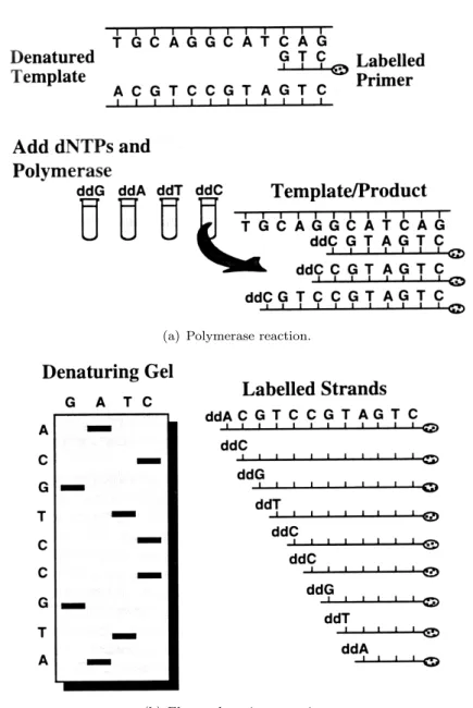
Genomic sequencing began with the development, by Frederic Sanger, of the Sanger sequencing, in the 1970s. This method, also known as dideoxynucleotide or chain termi-nation method [8], has been the only widely used technology for over three decades. In this technique, the DNA is used as a template to generate multiple copies of the same molecule that differ from each other in length, by a single base. The DNAs are then separated based on their size, and the bases at the end are identified, recreating the original DNA sequence (see Figure 2.3).
More specifically, in this method a single strained piece of DNA is amplified many times by the addition of dideoxy-nucleotides instead of deoxy-nucleotides. In fact, when the DNA is amplified, new deoxy-nucleotides (dNTPs) are usually added as the strand of DNA grows, but in the Sanger method this bases are replaced by special ones, called dideoxy-nucleotides (ddNTPs). There are two important differences that characterize the ddNTPs with respect to the similar dNTPs: they have fluorescent tags attached to them (a different tag for each of the 4 ddNTPs) and a crucial atom is missing, so that it prevents new bases from being added to a DNA strand, after that a ddNTP is added. This means that if during a DNA strand growth a ddNTP is inserted, the
synthesis process is stopped because no other nucleotides can be added after that, on the strand. If this amplification process is repeated for many cycles, as a result, all the possible lengths of DNA will be represented, and every piece of the synthesized DNA will contain a fluorescent label at its terminus (see Figure2.3(a)).
At this point, by using a gel electrophoresis, the amplified DNA can be separated ac-cording to its size. In this way, the DNA is separated from the smallest to the largest, and while the fluorescent DNA reaches the bottom of the gel, a laser can pick up the fluorescence of each piece of DNA. Each ddNTP (ddA, ddC, ddG, ddT) emits a different fluorescent signal that can be recorded on a computer, indicating the presence of a spe-cific ddNTP at the terminus. Since every possible size of DNA strand is present (each one with its terminating ddNTP), the DNA strand has a fluorescent ddNTP at every position, and this also means that every nucleotide in the strand can be determined. At this point a computer program can convert the data, read by the laser, into a coloured graph, showing the determined sequence (see Figure2.3(b)).
In the past, instead of using a computer, the resulting gel needed to be analyzed man-ually. This was a time consuming step, in fact the separation of the DNA strands by electrophoresis required the use of radioisotopes for labeling ddNTPs, one for each ddNTP (four different reactions). Today, thanks to all the improvements in fluorescent labels and in gel electrophoresis, DNA sequencing is fully automated (including the read out of the final sequence) and it is also faster and more accurate than before.
Sanger sequencing revolutionized the way in which the biology was studied, providing a way to learn the most basic genetic information. However, despite large efforts to improve the efficiency and the throughput of this technique, such as the development of automated capillary electrophoresis and computer driven assembly programs, the Sanger sequencing remained costly and time consuming, especially for applications involving the sequencing of whole genomes of organisms, such as humans.
2.3.2 Next Generation Sequencing
In the past few years a “revolution” occurred in the field of sequencing. This was due to the development of a number of new high-throughput sequencing technologies, known as Next-Generation Sequencing (NGS) technologies, that are now widely adopted [9].
These technologies have fundamentally changed the way in which we think about ge-netic and genomic research, opening new perspectives and new directions that were not achievable or even thinkable with the Sanger method. They have provided the opportu-nity for a global investigation of multiple genomes and transcriptomes, in an extremely
(a) Polymerase reaction.
(b) Electrophoretic separation.
Figure 2.3: Sanger sequencing process. Figure2.3(a)illustrates the products of the polymerase reaction, taking place in the ddCTP tube. The polymerase extends the la-beled primer, randomly incorporating either a normal dCTP base or a modified ddCTP base. At every position where a ddCTP is inserted, the polymerization terminates; the final result is a population of fragments. The length of each fragment represents the relative distance from the modified base to the primer. Figure2.3(b) shows the elec-trophoretic separation of the products of each of the four reaction tubes (ddG, ddA, ddT, and ddC), run in individual lines. The bands on the gel represent the respective fragments shown to the right. The complement of the original template (read from bottom to top) is given on the left margin of the sequencing gel.
efficient and timely manner at much lower costs, if compared with Sanger-based se-quencing methods. One of the main advantages offered by NGS technologies is their ability to produce an incredible volume of data, cheaply, that in some cases exceeds one billion of short reads per instrument run. Applications that have already benefitted from these technologies, include: polymorphism discovery [10], non-coding RNA discover [11], large-scale chromatin immunoprecipitation [12], gene-expression profiling [13], mutation mapping and whole transcriptome analysis.
One of the common technological features that is shared among all the available NGS platforms is the massively parallel sequencing of DNA molecules (single or clonally am-plified) that are spatially separated in a flow cell. In fact, the sequencing is performed by repeated cycles of polymerase-mediated nucleotide extensions or, in one format, by iterative cycles of oligonucleotide ligation.
In the following, the main available NGS systems will be described, analyzing technolo-gies and features of the instruments used for the sequencing process [14]. The most diffuse platforms are the ones produced by Roche/454 Life Sciences,Illumina and Life Technologies. In addition to these ones, there are also two emerging technologies: Ion Torrent and Pacific Biosciences.
Roche/454 Life Science
454 Life Sciences, founded in 2000 by Jonathan Rothberg, developed the first commer-cially available NGS platform, the GS 20, that was launched in 2005. This platform combined the single-molecule emulsion PCR with pyrosequencing, and was used by Margulies and colleagues to perform a shotgun sequencing of the entire 580,069bp of the Mycoplasma genitalia genome, resulting in a 96% coverage and 99.96% accuracy with a single GS 20 run. In 2007, Roche Applied Science acquired 454 Life Sciences, and introduced a second version of the 454 instrument, called GS FLX. In this new platform, that shared the same core technology of the GS 20, the flow cell is referred to as a “picotiter well” plate, which is made from a fused fiber-optic bundle.
The library of template DNAs used for sequencing is prepared by first cutting the molecule, and then end-repairing and ligating the obtained fragments (several hun-dred base pairs long) to adapter oligonucleotides. The library is then diluted to a single-molecule concentration, denatured, and hybridized to individual beads, contain-ing sequences complementary to adapter oligonucleotides. By uscontain-ing an emulsion PCR, the beads are then compartmentalized into water-in-oil mixture, where the clonal ex-pansions of single DNA molecules bound to the beads. The beads are deposited into individual picotiter-plate wells, and combined with sequencing enzymes (PTP loading).
Figure 2.4: Roche 454 sequencing. In the library construction, the DNA is fragmented
and ligated to adapter oligonucleotides, and then the fragments are clonally amplified by emulsion PCR. The beads are then loaded into picotiter-plate wells, where iterative pyrosequencing process is performed.
After that, thepyrosequencing is performed by successive flow additions of the 4 dNTPs: the four DNA nucleotides are added sequentially, in a fixed order across the picotiter-plate device, during a sequencing run. When a nucleotide flows, millions of copies of DNA bound to each of the beads and can be sequenced in parallel. In this way, each nucleotide complementary to the template strand is added into a well, and so the poly-merase extends the existing DNA strand with one nucleotide. A camera records the light signal emitted by the addition of one (or more) nucleotide(s) (see Figure2.4).
The two currently available systems by Roche/454 Life Sciences are the GS FLX+ and the GS Jr., which generate up to 1×10⁶ and 1×10⁵ reads per run, respectively. More specifically, there are two instruments using the first system (GS FLX+), that are: the GS FLX Titanium XLR70 and the newest GS FLX Titanium XL+. These two instruments produce reads of length 450 and 700 base pairs respectively, with a typical throughput of 450Mb in 10 hours for the first instrument, and 700Mb in 23 hours for the second, both maintaining an error rate <1%. On the other hand, the GS Jr. system produces reads of length∼400 base pairs, for a throughput of∼35Mb in 10 hours, with an error rate of<1%. Table2.1summarizes all the previous information onRoche/454 Life Sciences instruments.
Instrument Read length Throughput Run time (bp) (Mb/run) (hours)
GS FLX Titanium XLR70 450 450 10
GS FLX Titanium XL+ 700 700 23
GS Jr. system ∼400 ∼35 10
Table 2.1: Roche/454 Life Sciences NGS instruments. Illumina/Solexa
Solexa was founded in 1998 by two British chemists, Shankar Balasubramanian and David Klenerman, and the first short read sequencing platform, called Solexa Genome Analyzer, was launched in 2006. In the same year the company was acquired byIllumina.
The process of sequencing in the Genome Analyzer system is done by cutting the DNA molecule into small fragments (several hundred base pairs long) and, after that, oligonu-cleotide adapters are added to the ends of the these fragments to prepare them for the binding to the flow cell (see Figure2.5(a)). This latter cell consists of an optically trans-parent slide with 8 individual lanes on the surface, on which oligonucleotide anchors are bound. When the single-stranded template DNAs are added to the flow cell, they are immobilized by hybridization to these anchors (see Figure 2.5(b)). Once the strand is attached to an anchor primer, it is “arched” over and hybridized to an adjacent anchor oligonucleotide (that has a complementary primer) by a “bridge” amplification in the flow cell (see Figure 2.5(c)). Starting from the primer on the surface, the DNA strand is replicated in order to create more copies (see Figure 2.6(a)), that are than denatured (see Figure2.6(b)). At this point, starting from a single-strand DNA template, multiple amplification cycles are performed, in order to obtain a “cluster” (of about a thousand copies) of clonally amplified DNA templates (see Figure 2.6(c)). Before starting the sequencing process, the clusters are washed, leaving only the forward strands (to make the sequencing more efficient). To start the sequencing process, primers complementary to the adapter sequences, polymerase and a mixture of 4 differently colored fluorescent reversible dye terminators are added to the mix. In this way, the added primers are bound to the primers of the strand and the terminators are incorporated, according to sequence complementarity of each strand present in the clonal cluster (see Figure2.7(a)). As bases are incorporated, a laser is used to activate the fluorescence (see Figure2.7(b)) and the color is read by a computer, obtaining the sequence from many clusters (see Figure2.7(c)). This iterative process, calledsequencing by synthesis, takes more than 2 days to generate a read sequence, but, since there are millions of clusters in each flow cell, the overall output is>1 billion base pairs (Gb) per run.
(a) DNA sample preparation. (b) Binding to the surface. (c) Bridge amplification.
Figure 2.5: Illumina sequencing 1/3. The DNA sample is fragmented and the adapters are bound to the ends (Figure 2.5(a)); the obtained single-strained fragments are attached to the flow cell surface (Figure 2.5(b)) and then they are “bridged” (Fig-ure2.5(c)).
(a) Double-strained fragments. (b) Denaturation. (c) Amplification.
Figure 2.6: Illumina sequencing 2/3. The fragments become double-strained
(Fig-ure2.6(a)) and then they are denatured. This process leaves anchored single-strained fragments (Figure 2.6(b)). After a complete amplification, millions of clusters are formed on the flow cell surface (Figure2.6(c)).
(a) First base determination. (b) Iterative sequencing process. (c) Sequence reading.
Figure 2.7: Illumina sequencing 3/3. The clusters are washed, leaving only the
forward strands and, to initiate the sequencing process, primer, polymerase and a 4 colored terminators are added. The primers are bound to the primers of the strand and, after that, the first terminator is incorporated (Figure 2.7(a)). By iterating the incorporation process, all the sequence nucleotides are added and the laser activates the fluorescence (Figure2.7(b)). During the incorporation a computer reads the image and determines the sequence of bases (Figure2.7(c)).
Instrument Read length Throughput Run time (bp) (Gb/run) (days)
HiSeq 2000 2×100 600 11
GAIIx 2×150 95 14
MiSeq 2×150 2 1
Table 2.2: Illumina/Solexa NGS instruments.
The newest platforms can analyze higher cluster densities and have been improved in the sequencing chemistry allowing to obtain longer reads. Currently, there are 3 types of available instruments by Illumina, all producing paired-end read (see Section 2.4). More specifically, the HiSeq 2000 system can generate about 600 Gb of 2×100 base pair reads for run, taking an overall time of about 11 days. There are also other models of this instrument that have the possibility to perform “rapid runs”, in order to obtain a smaller amount of reads in less time. Similarly to the previous instrument, the Genome Analyzer IIx (GAIIx) can produce up to 95 Gb of 2×150 base pair reads per single flow cell, taking about 14 days. Finally, the MiSeq instrument can produce reads of the same size of the previous one (2×150 base pairs), but with a throughput of 2 Gb in about one day. The information about these instruments are summarized in Table2.2.
Life Technologies
Life Technologies was formed in 2008 by the merging of Invitrogen and Applied Biosys-tem; to be more precise, the former company bought the latter, and the two became Life Technologies. It was in 2007 that Applied Biosystem refined the technology of SOLiD (Supported Oligonucleotide Ligation and Detection) System 2.0 platform, previously developed in the laboratory of George Church, and released its first NGS system, the SOLiD instrument.
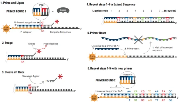
As for Roche/454 technology, the sample preparation consists of DNA fragments that are then ligated to oligonucleotide adapters; after that, the fragments are attached to beads and are clonally amplified by an emulsion PCR. Finally, beads with clonally amplified template are immobilized onto a derivitized-glass flow-cell surface, where the sequencing process starts. The major difference between SOLiD and the other NGS platforms is its sequencing by ligation (instead of sequencing by synthesis). The sequencing by ligation process starts by annealing a sequencing primer, complementary to the adapter at the “adapter–template” junction, and adding a mixture of all the 16 possible probes. In the specific, probes involved in this sequencing process are used to detect two adjacent bases (16 possible combinations), but there are only 4 different fluorescent dyes. Because of this, each base in the sequence is interrogated twice in order to obtain the correct original sequence (see Figure 2.9). Once the primer is annealed, the correct di-base probe, i.e. the one with the first two bases complementary to the first two bases of the template sequence, binds to this latter template and ligates to the primer (see Figure 2.8(1)). Each probe is an octamer, which consists of (3’-to-5’ direction) 2 probe-specific bases followed by 6 degenerate bases (denoted asnnnzzz) with one of the 4 fluorescent labels linked to the 5’ end. After the ligation of the probe, the fluorescence signal is recorded (see Figure2.8(2)) and then the last 3 degenerated bases are cleaved and washed in order to obtain the new 5’ phosphate group that is used to ligate the probe in the next cycle (see Figure 2.8(3)). To extend the first primer, seven cycles of ligation, referred to as a round, are performed (see Figure2.8(4)) and then this synthesized strand is denatured. At this point, the new round is started, and a new sequencing primer, which is shifted of one base with respect to the previous one, is annealed. This latter has an offset of (n−1) with respect to the original template sequence (see Figure 2.8(5)). The overall sequencing process is composed of five rounds, each of which is performed with a new primer and with successive offsets (n−2,n−3 andn−4) (see Figure2.8(6)).
One of the main features of this sequencing process is that the perfect annealing of the probes is controlled by 2 bases of oligonucleotides. Thus, this method is usually more accurate and specific than the sequencing by synthesis approaches. Currently, there are 2 available NGS instruments by Life Technologies. The first, the SOLiD 4 system, can
Figure 2.8: Sequencing by ligation. In (1) the primer is annealed to the adaptor and
the first two bases of the probe are bound to the first two bases of the sequence. The fluorescence signal is read (2) and the last bases of the probe are cleaved, so that the new phosphate group is created (3). This ligation process is repeated for seven cycles (4), in order to extend the primer. Finally, this latter primer is melted off and a new one is annealed (5). The previous steps are repeated for all the new primers, with different offsets (6).
Figure 2.9: Summary of the sequencing by ligation process showing, for each base of
the read sequence, the positions of the interrogations (2 for each position).
produce up to 100 Gb of 2×50 mate pair reads, in about 12 days. In a similar way, the second one, called SOLiD 5500xl system, can produce up to 180 Gb of 75×35 base pairs (paired-end) or 60×60 base pairs (mate-paired), in about 7 days. All the previous information onLife Technologies instruments are summarized in Table2.3.
Instrument Read length Throughput Run time (bp) (Gb/run) (days)
SOLiD 4 2×50 100 12
SOLiD 550xl 75×75 (paired) 180 7 60×60 (mate)
Table 2.3: Life Technologies/SOLiD NGS instruments. Emerging Technologies
In addition to the previously described methods, there are also some other new emerging technologies, in the sequencing field. In the following, two of them will be briefly pre-sented. The first one is the so called Ion Torrent technology, in which the information coming from the chemical sequence is translated into digital form, without any fluores-cence. In fact, this method relies on a well known biochemical process: in nature, when a nucleotide is incorporated into a strand of DNA by a polymerase, a hydrogen ion (H+) is released as a byproduct. This hydrogen ion carries a charge that the system’s ion sensor can detect. This sensor is composed of a high-density array micro-machined wells that allow to perform biochemical processes in a parallel manner. In this way, when a nucleotide is incorporated into a DNA strand, it releases a hydrogen ion which charges the pH of the solution. This charge can be detected by the ion sensors and translated into digital form. Any nucleotide that is added to a DNA template is detected as a voltage change, and if a nucleotide is not a match for a particular template, no voltage change will be detected and no base will be called for that template. On the other hand, if there are two identical bases on the DNA strand, the voltage is doubled, and the chip records two identical base calls. Thanks to this new technology, it is possible to reach a throughput of 1 Gb in a few hours, depending on the used chip. Moreover, this technology is still under development in order to improve the read quality and increase the length of the produced sequences.
In addition to the previous one,Pacific Biosciencesdeveloped a single-molecule real-time (SMRT) sequencing system. This technology uses a progressive sequencing by synthesis in which the nucleotides, incorporated during the polymerase, have a fluorescent dye at-tached to the poly-phosphate chain (phospholinked-nucleotides). Such dyes are different for each of the 4 bases. The sequencing is performed on the SMRT cells, which contain thousand of zero-mode waveguides (ZMWs), providing a visualization chamber. In this way, when a base is incorporated, the fluorescent nucleotide is brought into the poly-merase’s active site and a high-resolution camera, in the ZMW, records this fluorescence signal. In addition to this, since the sequencing library is prepared in such a way that the resulting molecule is circular, it is possible to sequence the template using a scheme, called circular consensus sequencing, that improves the accuracy of the base calls, by
using the redundant sequencing information. This system gives the longest reads, in fact, the average read length per run is around 1.5 Kb. These, are two of the currently emerging technologies, that are continuously evolving in the field of sequencing, and are usually referred to as Third Generation Sequencing (TGS) technologies.
2.4
Data
NGS technologies have overcame the limitations of the previous sequencing methods by providing a new “kind” of data, suited for answering a wide range of biological questions. More specifically, one of the features that is shared among all the previously illustrated platforms, is that they produce a huge quantity of short sequences (short reads) that deeply cover the sequenced molecule. In the following, the main features of NGS technologies will be described.
The first, and probably the most relevant observation, is done by comparing the produced NGS reads to the ones of classical methods, such as Sanger sequencing, in terms of sequence length. In fact, depending on the adopted platform, the produced sequences can range from 35 base pairs of the Illumina machines, to several hundred base pairs of the Roche/454 systems, which are still shorter than the sequences, few thousand base pairs long, of the Sanger method. Another key point of this new generation of systems is the throughput, that is much higher than before. Due to such a massive amount of involved data, the management and the analysis of the data require dedicated software and also high-performance and capacity computing resources. This shift, from a low number of long reads to a huge number of short reads, can be also observed from a coverage point of view, which is the average number of reads that represent (cover) a given nucleotide, in the original sequence. In the classical methods, the typical coverage was 1x - 2x, meaning that each base was present in at most two reads. On the other hand, with the advent of the NGS technologies, it is now possible to reach a coverage of 10x or 100x of the given sequence, which correspond to an improvement of one or two orders of magnitude.
It is not easy to directly compare the different NGS platforms, especially from an error rate point of view. In fact, for example, most of the times the value reported by the companies is based on sequence reads of particular templates, that are favourable for their platform. However, in almost all the previously introduced instruments (except the one by Pacific Biosciences), the errors increase near the end of each platform’s maximum read length. Indeed, maximum read length is limited by error tolerance. Although the error rate comparison is difficult for other reasons, in Table 2.4 are reported the “reasonable approximations” that can be used to compare different platforms [15].
Instrument Primary Single-pass Final Errors Error Rate (%) Error Rate (%)
454 - all Models Indel 1 1
Illumina - all models Substitution ∼0.1 ∼0.1
SOLiD 5500xl A-T bias ∼5 60.1
Ion Torrent - all chips Indel ∼1 ∼1 Pacific Biosciences CG Deletion ∼15 615
Table 2.4: Error rate comparison of different sequencing platforms. Phred Probability of Base Call Quality Score Incorrect Base Call Accuracy
10 1 in 10 90%
20 1 in 100 99%
30 1 in 1,000 99.9%
40 1 in 10,000 99.99% 50 1 in 100,000 99.999%
Table 2.5: Quality score and base calling accuracy.
From Table2.4, it is possible to notice that the error rate varies from 0.1% of the SOLiD 5500xl and Illumina systems, to 15% of the Pacific Biosciences one. These values are referred to the final error rate, which can be different from the one obtained in a single passage. This is the case of SOLiD, that has the second highest raw error rate (∼5%), but, by allowing a double or triple encoding of each base (i.e. each base is sequenced independently two or three times, with inconsistent data becoming inaccessible to users), it achieves its low error rate (60.1%). In a similar way, Illumina refers its error rate not on the entire data, reaching a∼0.1%; also Pacific Biosciences suggests of reading each template multiple times, in order to overcome high error rates and to achieve a consensus sequence with a low error rate, but it gives users the option to obtain single-pass data. Finally, in addition to raw error rates of sequencing reads, each platform has also its own biases. To this purpose, each sequencing platform usually provides the quality of the produced data, by adding an extra information in the read file (or in a separated one), about the quality of each base present in the sequences. For each nucleotide, it is used the Phred quality score as a measure of reliability. This measure, denoted as Q, is logarithmically related to the base-calling error P:
Q=−10 log10P
whereQis the phred quality score andP is the probability that the base call is incorrect. This means that, the smaller theP, the higher theQ. From another point of view, 1−P
is the probability of correctness of the base, so ifP = 0.01, then the quality scoreQ= 20 and the probability that is correct is 0.99 (i.e. 99%) (see Table 2.5).
The “old way” to provide the information about the sequences and the associated quality values was to provide two separated files. The first one, inFASTAformat, in which there were the sequences, and the other one, containing the phred values:
FASTA Sequence file :
>SEQ ID agtcTGATATGCTgtacCTATTATAATTCTAGGCGCTCATGCCCGCGGATATCGTAGCTA Quality file : >SEQ ID 10 15 20 22 50 50 50 50 50 50 50 50 50 50 50 50 50 50 50 50 50 50 50 20 50 50 50 14 50 50 50 11 20 25 25 30 30 20 15 20 35 50 50 50 50 50 50 50 50 50 50 50 50 50 50 50 50 50 50 50
In the specific, in a FASTA file there are two lines for each entry, i.e. for each read: the first one contains the read id (prefixed with>) and the second one contains the sequence of the read. The quality file adopts the same format, but instead of the nucleotides, the second line is a sequence of numeric values, one for each base of the read in the FASTA file, indicating the quality score. To have a more compact way to provide the information about read and quality scores, a new format has been adopted. This “new way”, called FASTQ, incorporates both the information in a single file. In the specific, it is organized as: FASTQ file : @SEQ ID GATTTGGGGTTCAAAGCAGTATCGATCAAATAGTAAATCCATTTGTTCAACTCACAGTTT + !’’*(((***+))%%%++)(%%%%).1***(-+*(’’))**55CCF>>>>>>CCCCCCC65
In the first line of each entry, the sequence identifier starts with the ’@’ symbol (instead of ’>’) and it is followed by the sequence in another line (as in the FASTA file). After that, there is a separator line started with a symbol (which usually is ’+’), and finally, there is a line containing the encoded quality values (one symbol per nucleotide). The fourth line encodes the quality values of the sequence of nucleotides present in the second line, and obviously, it must contain the same number of symbols as the number of letters of the sequence. The quality encoding is done by using letters and symbols to represent numbers, and the range of adopted symbols depends on the used platform. The following example refers to the Illumina range of symbols, with associated quality scores from 0 to 41:
! " # $ % & ’ ( ) * + , - . / 0 1 2 3 4 5 6 7 8 9 : ; < = > ? @ A B C D E F G H I J
| | | | |
Q0 Q10 Q20 Q30 Q40
For this reason, one of the first steps in an analysis pipeline that uses NGS data is the sequencing filter, based on the phred values, in order to discard the reads with poor qualities or to cut them at a certain length (read trimming).
As a final remark, all the NGS platforms, in addition to the “single” short read sequences, offer the possibility to producepaired-endreads, i.e. sequences that are derived from both the ends of the fragment, in the library. Obviously, there are some differences among read pairs, depending from the used platform. In particular, it is possible to distinguish between:
• Paired-ends, that are a linear fragment sequenced at both the ends in two separate reactions;
• Mate-pairs, that are a circularized fragment, usually>1 Kb long, sequenced by a single reaction or by two separate end reads.
In general, paired-end reads offer some advantages, e.g. for the sequencing of large and complex genomes, because they can be more accurately placed (mapped), than the single ended short reads and so they can be used to disambiguate some complex situations. It is also possible to distinguish reads that are coming from cDNAs, that carry information about RNA molecules. In this case they are calledRNA-Seq reads.
2.4.1 RNA-Seq
The RNA sequencing method, called RNA-Seq, is the use of the previously described technologies, for the sequencing RNA molecules [16]. This technique has revolutionized the way in which transcriptomes are analyzed, providing a new approach to map and quantify them. As said, by using NGS technologies, a population of RNAs is converted into a library of cDNA fragments by attaching adaptors to the ends of each sequence. These fragments are then sequenced, obtaining a set of short reads (or paired-ends reads).
RNA-Seq has opened new prospectives, like the possibility of identifying the positions of the transcription boundaries. In fact, novel transcribes regions and introns for ex-isting genes can be annotated, and moreover, some of the aspects of the exex-isting gene annotations can be modified and corrected. In addition to this, the information about
the connection of two or more exons can be obtained by using short and long reads. For these reasons, RNA-Seq is particularly suited for studying complex transcriptomes, to reveal sequence variations. Furthermore, from a quantitative point of view, RNA-Seq can be used to determine the expression levels of RNA molecules, in a more accurate way, than in the previous methods. Considering all the mentioned advantages, RNA-Seq has generated a global view of the transcriptome and its composition for a number of species (known or unknown) and has revealed new splicing isoforms of many genes.
The annotation of alternative splicing variants and events, to differentiate and compare organisms, is part of the central goal in transcriptome analysis of identifying and quan-tifying all full-length transcripts. RNA-Seq will help to reach this purpose. It can also be applied to the biomedical field, in order to compare normal and diseased tissues to understand the physiological changes between them. Another challenge, involving RNA-Seq, is its use to target complex transcriptomes, in order to identify rare RNA isoforms from the genes. In the near future, RNA-Seq is expected to replace microarrays for many applications involving the structure and the dynamic of transcriptomes.
2.5
Definitions
2.5.1 Strings
Lets=s1s2· · ·s|s|be a sequence of characters over the alphabet Σ, that is astring. The
length of the stringsis denoted by|s|and thesizeof Σ is denoted by|Σ|. If considering DNA molecules, the typical alphabet is Σ = {A, C, G, T}, wherex ∈ Σ is a nucleotide and the length is measured in the number of nucleotides (nt), orbase pairs (bp) when referring to the double stranded molecule. Theith character of a stringsis denoted by
s[i]. Then s[i: j] denotes the substring sisi+1· · ·sj of s, while s[: i] and s[j :] denote
respectively the prefix of sconsisting of isymbols and the suffix of sstarting with the
j-th symbol ofs.
We denote with pre(s, i) and suf(s, i) respectively the prefix and the suffix of lengthiof
s. Among all prefixes and suffixes, we are especially interested into LH(s) = pre(s,|s|/2) and RH(s) = suf(s,|s|/2) which are called the left half and theright half of s.
Given two strings s1 and s2, the overlap ov(s1, s2) is the length of the longest suffix
of s1 that is also a prefix of s2. The fusion of s1 and s2, denoted by ϕ(s1, s2), is the
string s1[:|s1| −ov(s1, s2)]s2 obtained by concatenating s1 and s2 after removing from s1 its longest suffix that is also a prefix of s2. We extend the notion of fusion to a
G= ( V ={1,2,3,4,5}, E={(1,2),(1,3),(1,4),(1,5),(2,3),(2,4),(4,5)} ) 1 2 3 4 5
(a) Example of Undirected Graph. G= ( V ={1,2,3,4,5}, E={(1,2),(1,5),(2,3),(2,4),(3,2),(4,1),(4,5)} ) 1 2 3 4 5
(b) Example of Directed Graph.
Figure 2.10: Examples of graphs. Both the graphs have 5 nodes and 7 edges, but in
Figure2.10(a)the edges are unordered (i.e. (u, v) = (v, u)) and they are represented as simple lines. Instead in Figure 2.10(b) the edges are ordered (i.e. (u, v)6= (v, u)) and they are represented as arrows indicating the direction.
sequence of strings hs1, . . . , ski as ϕ(hs1, . . . , ski) = ϕ(s1, ϕ(hs2, . . . , ski)) if k >2, and ϕ(hs1, s2i) =ϕ(s1, s2).
2.5.2 Graphs and Trees
Graphs
A graph Gis an ordered pair (V, E), where V is a finite set called the vertex set and E
is called the edge set. Given two vertexes (or nodes) u, v∈V, an edge (or arc) is a pair (u, v) ∈E. An edge e= (u, v) is directed if one endpoint is the “head” and the other the “tail” (making eordered, i.e. (u, v) 6= (v, u)). In such a case the graph G is called directed graph (ordigraph). Otherwise, if there is no direction in the edges, the graph is called undirected graph (see Figure 2.10 for an example of graphs). If (u, v) is an edge in a directed graphG= (V, E),eisincident from (oroutgoing) vertexuand is incident to (or ingoing) vertex v. If (u, v) is an edge in an undirected graph G = (V, E), e is incident to vertexesu and v. Given a vertex v∈V, the indegree of v is the number of its ingoing edges and the outdegree is the number of its outgoing edges. In a directed graph the degree of a vertex is the sum of its indegree and its outdegree edges, instead in an undirected graph the degree of a vertex is the number of edges incident on it.
A path (or walk) of length k from a vertex u to a vertex u0 in a graph G = (V, E) is a sequence hv0, v1, . . . , vki of vertexes such that u =v0, u0 = vk and (vi−1, vi) ∈ E for i= 1, . . . , k. The length of the path is the number of edges in the path. A path forms a cycle if its endpoints u and u0 are the same, i.e. u = u0. A graph is called acyclic if it contains no cycles. A graph that is directed and acyclic is called directed acyclic
graph (DAG). A graphG0 = (V0, E0) is asubgraph of G= (V, E) ifV0⊆V andE0 ⊆E. Given a set V0 ⊆ V, the subgraph induced by V0 is the graph G0 = (V0, E0), where
E0 ={(u, v)∈E :u, v∈V0}. An undirected graph is connected if every pair of vertexes is connected by a path, and aconnected component is a maximal connected subgraph of the graph. A connected graph has one connected component.
An interesting and well studied type of graphs are the so calledDe Bruijn graphs. This latter graphs were initially developed to find the shortest cyclic sequence of letters from an alphabet, in which every possible string of length k appears as a substring in the cyclic sequence. To construct such a graph, given an alphabet Σ, all possible (k− 1)-mers (substrings of length k−1) are assigned to nodes, and there exists a direct edge between two (k−1)-mers, x and y, if there is somek-mer whose prefix is x and whose suffix is y. In this way, the k-mers are represented by the edges of the graph. All the possible substrings of length k of an alphabet Σ are |Σ|k. For example, if dealing with
the DNA, the usual alphabet is Σ = {A, C, G, T} and so all the possible substrings of length k are 4k. In the binary alphabet (i.e. Σ = {0,1}) all the possible substrings of length 3 are (23 = 8): 000, 001, 010, 011, 100, 101, 110, 111. The corresponding De Bruijn graph with k = 4, that has all the previous substrings as nodes, is shown in Figure2.11. Eachk-mer can be obtained by taking the (k−1)-mer at the starting node and overlapping the (k−1)-mer at the ending node. It must be also noticed that two consecutive nodes (i.e. nodes that are connected by an edge) have an overlap of k−2 (i.e. the suffix of lengthk−2 of the first one is equal to the prefix of lengthk−2 of the second one).
This type of graphs have been recently used for the assembly of sequences from NGS data in order to provide an efficient approach to solve that computational problem. One of the differences, with respect to the formulation of the problem for which theDe Bruijn graphswere initially developed, is that, when dealing with short reads, not all the possible substrings of lengthk of a given alphabet are present. The advantage of using De Bruijn graphs is that the sequence can be reconstructed by an Eulerian cycle (in the example in Figure 2.11 the shortest circular sequence, that contains all the 4-mers as substrings, is 0000111101100101).
Trees
A (free)tree is a connected, acyclic, undirected graph. LetG= (V, E) be an undirected graph. The following statements are equivalent.