Question answering with textual sequence matching

Singapore Management University

Institutional Knowledge at Singapore Management University

4-2019

Question answering with textual sequence

matching

Shuohang WANG

Singapore Management University, [email protected]

Follow this and additional works at:https://ink.library.smu.edu.sg/etd_coll

Part of theDatabases and Information Systems Commons, and theTheory and Algorithms Commons

This PhD Dissertation is brought to you for free and open access by the Dissertations and Theses at Institutional Knowledge at Singapore Management University. It has been accepted for inclusion in Dissertations and Theses Collection (Open Access) by an authorized administrator of Institutional Knowledge at Singapore Management University. For more information, please [email protected].

Citation

WANG, Shuohang. Question answering with textual sequence matching. (2019). Dissertations and Theses Collection (Open Access).

QUESTION ANSWERING WITH TEXTUAL

SEQUENCE MATCHING

SHUOHANG WANG

SINGAPORE MANAGEMENT UNIVERSITY

2019

Question Answering with Textual

Sequence Matching

by

Shuohang WANG

Submitted to School of Information Systems in partial fulfillment of the requirements for the Degree of Doctor of Philosophy in Information Systems

Dissertation Committee:

Jing Jiang (Supervisor / Chair)

Associate Professor of Information Systems Singapore Management University

Baihua Zheng

Associate Professor of Information Systems Singapore Management University

David _Lo

Associate Professor of Information Systems Singapore Management University

Wei Lu

Assistant Professor of Information Systems Technology and Design

Singapore University of Technology and Design

Singapore Management University

2019

I hereby declare that this PhD dissertation is my original work

and it has been written by me in its entirety.

I have duly acknowledged all the sources of information which

have been used in this dissertation.

This PhD dissertation has also not been submitted for any

degree in any university previously.

Shuohang Wang

16 April 2019

Question Answering with Textual

Sequence Matching

Shuohang Wang

Abstract

Question answering (QA) is one of the most important applications in natural language processing. With the explosive text data from the Internet, intelli-gently getting answers of questions will help humans more efficiently collect useful information. My research in this thesis mainly focuses on solving ques-tion answering problem with textual sequence matching model which is to build vectorized representations for pairs of text sequences to enable better reasoning. And our thesis consists of three major parts.

In Part I, we propose two general models for building vectorized represen-tations over a pair of sentences, which can be directly used to solve the tasks of answer selection, natural language inference, etc.. In Chapter 3, we propose a model named “match-LSTM”, which performs word-by-word matching fol-lowed by a LSTM to place more emphasis on important word-level matching representations. On the Stanford Natural Language Inference (SNLI) [7] cor-pus, our model achieved the state of the art. Next in Chapter 4, we present a general “compare-aggregate” framework that performs word-level matching followed by aggregation using Convolutional Neural Networks. We focus on exploring 6 different comparison functions we can use for word-level matching, and find that some simple comparison functions based on element-wise oper-ations work better than standard neural network and neural tensor network based comparison.

In Part II, we make use of the sequence matching model to address the task of machine reading comprehension, where the models need to answer the question based on a specific passage. In Chapter 5, we explore the power of

word-level matching for better locating the answer span from the given passage for each question in the task of machine reading comprehension. We propose an end-to-end neural architecture for the task. The architecture is based on match-LSTM and Pointer Net which constrains the output tokens coming from the given passage. We further propose two ways of using Pointer Net for our tasks. Our experiments show that both of our two models substantially outperform the best result [61] using logistic regression and manually crafted features. Besides, our boundary model also achieved the best performance on the SQuAD [61] and MSMARCO [57] dataset. In Chapter 6, we will explore another challenging task, multi-choice reading comprehension, where several candidate answers are also given besides the question related passage. We propose a new co-matching approach to this problem, which jointly models whether a passage can match both a question and a candidate answer.

In Part III, we focus on solving the problem of open-domain question an-swering, where no specific passage is given any more comparing to the reading comprehension task. Our models for solving this problem still rely on the textual sequence matching model to build ranking and reading comprehension models. In Chapter 7, we present a novel open-domain QA system called Re-inforced Ranker-Reader (R3), which jointly trains the Ranker along with an answer-extraction Reader model, based on reinforcement learning. We report extensive experimental results showing that our method significantly improves on the state of the art for multiple open-domain QA datasets. As this work can only make use of a single retrieved passage to answer the question, in the next Chapter 8, we propose two models, strength-based re-ranking and

coverage-based re-ranking, which make use of multiple passages to generate their answers. Our models have achieved state-of-the-art results on three public open-domain QA datasets: Quasar-T [23], SearchQA [24] and the open-domain version of TriviaQA [40], with about 8 percentage points of improvement over the former two datasets.

Table of Contents

1 Introduction 1

1.1 Overview . . . 1

1.2 Thesis Outline and Contributions . . . 7

1.2.1 Textual Sequence Matching . . . 7

1.2.2 Machine Reading Comprehension . . . 8

1.2.3 Open-Domain Question Answering . . . 9

2 Related work 12 2.1 Textual Sequence Matching . . . 12

2.2 Machine Reading Comprehension . . . 13

2.2.1 Datasets . . . 13

2.2.2 End-to-end Neural Network Models for Machine Com-prehension . . . 14

2.3 Open-domain Question Answering . . . 14

I

General Textual Sequence Matching Models

17

3.2 Model . . . 20

3.2.1 Neural Attention Model . . . 20

3.2.3 Implementation Details . . . 25 3.3 Experiments . . . 26 3.3.1 Experiment Settings . . . 26 3.3.2 Main Results . . . 28 3.3.3 Further Analyses . . . 29 3.4 Conclusions . . . 34

4 A Compare-Aggregate Model for Textual Sequence Matching 35 4.1 Introduction . . . 35

4.2 Method . . . 38

4.2.1 Problem Definition and Model Overview . . . 39

4.2.2 Preprocessing and Attention . . . 41

4.2.3 Comparison . . . 42

4.2.4 Aggregation . . . 44

4.3 Experiments . . . 44

4.3.1 Task-specific Model Structures . . . 45

4.3.2 Baselines . . . 47

4.3.3 Analysis of Results . . . 49

4.3.4 Further Analyses . . . 50

4.4 Conclusions . . . 51

II

Machine Reading Comprehension with Textual

Se-quence Matching

52

5.2 Method . . . 56

5.2.1 Match-LSTM . . . 56

5.2.2 Pointer Net . . . 57

5.3 Experiments . . . 63 5.3.1 Data . . . 63 5.3.2 Experiment Settings . . . 64 5.3.3 Results . . . 64 5.3.4 Further Analyses . . . 67 5.4 Conclusions . . . 70

6 Multi-choice Reading Comprehension Using A Co-Matching Model 71 6.1 Introduction . . . 71 6.2 Model . . . 74 6.2.1 Co-matching . . . 75 6.2.2 Hierarchical Aggregation . . . 76 6.2.3 Objective function . . . 77 6.3 Experiment . . . 78 6.4 Conclusions . . . 80

III

Open-domain Question Answering with Textual

Sequence Matching Model

82

7.5.1 Overall Results . . . 96

7.5.2 Further Analysis . . . 96

7.6 Conclusion . . . 100

8 Evidence Aggregation for Answer Re-Ranking in Open-Domain Question Answering 101 8.1 Introduction . . . 101

8.2 Method . . . 105

8.2.1 Evidence Aggregation for Strength-based Re-ranker . . . 106

8.2.2 Evidence Aggregation for Coverage-based Re-ranker . . . 107

8.2.3 Combination of Different Types of Aggregations . . . 111

8.3 Experimental Settings . . . 112

8.3.1 Datasets . . . 112

8.3.2 Baselines . . . 113

8.3.3 Implementation Details . . . 114

8.4 Results and Analysis . . . 114

8.4.1 Overall Results . . . 114

8.4.2 Analysis . . . 115

8.5 Conclusions . . . 120

List of Figures

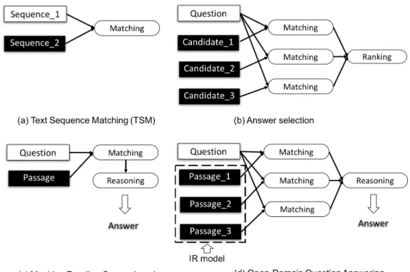
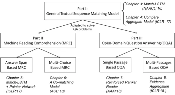
1.1 An overview of the frameworks for different question answering tasks. . . 5 1.2 An overview of the major components in the thesis. . . 6

3.1 The top figure depicts the model by Rockt¨aschel et al. (2016) and the bottom figure depicts our model. Here Hs _represents

all the hidden states hs

j. Note that in the top model each hak

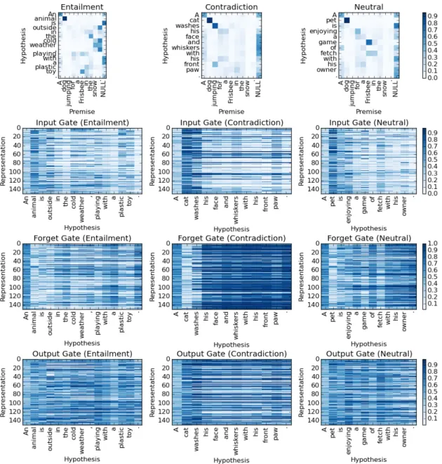
represents a weighted version of the premise only, while in our model, each hm_k represents the matching between the premise and the hypothesis up to positionk. . . 23 3.2 The alignment weights and the gate vectors of the three examples. 30

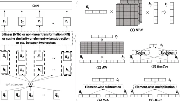
4.1 The left hand side is an overview of the model. The right hand side shows the details about the different comparison functions. The rectangles in dark represent parameters to be learned. ×

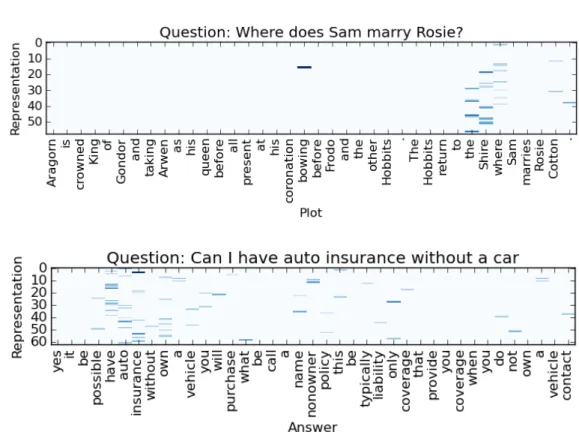
represents matrix multiplication. . . 39 4.2 An visualization of the largest value of each dimension in the

convolutional layer of CNN. The top figure is an example from the dataset MovieQA with CNN window size 5. The bottom figure is an example from the datasetInsuranceQAwith CNN window size 3. Due to the sparsity of the representation, we show only the dimensions with larger values. The dimensionality of the raw representations is 150. . . 50

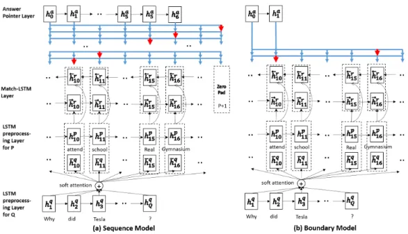
5.1 An overview of our two models. Both models consist of an LSTM preprocessing layer, a match-LSTM layer and an Answer Pointer layer. For each match-LSTM in a particular direction, ¯

hq_i, which is defined as Hqα|_i, is computed using the α in the corresponding direction, as described in Eqn. (5.2) . . . 58 5.2 Performance breakdown by answer lengths and question types

on SQuAD development dataset. Top: Plot (1) shows the per-formance of our two models (where s refers to the sequence model , b refers to the boundary model, and e refers to the ensemble boundary model) over answers with different lengths. Plot (2) shows the numbers of answers with different lengths. Bottom: Plot (3) shows the performance our the two models on different types of questions. Plot (4) shows the numbers of different types of questions. . . 67 5.3 Visualization of the attention weightsα for four questions. The

first three questions share the same paragraph. The title is the answer predicted by our model. . . 68

6.1 An overview of the model that builds a matching representation for a triplet {P,Q,A} (i.e., passage, question and candidate answer). . . 74

7.1 Overview of training our model, comprising a Ranker and a Reader based on Match-LSTM as shown on the right side. The Ranker selects a passage τ and the Reader predicts the start and end positions of the answer inτ. The reward for the Ranker depends on similarity of the extracted answer with the ground-truth answer ag. To accelerate Reader convergence, we also sample several negative passages without ground-truth answer. . 87

8.1 Two examples of questions and candidate answers. (a) A question benefiting from the repetition of evidence. Correct answer A2 has multiple passages that could support A2 as answer. The wrong an-swer A1 has only a single supporting passage. (b) A question ben-efiting from the union of multiple pieces of evidence to support the answer. The correct answer A2 has evidence passages that can match both the first half and the second half of the question. The wrong answer A1 has evidence passages covering only the first half. . . 103 8.2 An overview of the full re-ranker. It consists of strength-based

and coverage-based re-ranking. . . 106 8.3 Performance decomposition according to the length of answers

List of Tables

1.1 Examples for three different question answering tasks. . . 2

3.1 Experiment results in terms of accuracy. d is the dimension of the hidden states. |θ|W+M is the total number of parameters

and |θ|M is the number of parameters excluding the word

em-beddings. Note that the five models in the last section were implemented by us while the other results were taken directly from previous papers. Note also that for the five models in the last section, we do not update word embeddings so|θ|W+Mis the

same as |θ|M. The three columns on the right are the

accura-cies of the trained models on the training data, the development data and the test data, respectively. . . 26 3.2 The confusion matrix of the results by mLSTM with d = 300.

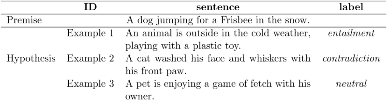
N,E andC correspond toneutral,entailmentandcontradiction, respectively. . . 28 3.3 Three examples of sentence pairs with different relationship

la-bels. The second hypothesis is a contradiction because it men-tions a completely different event. The third hypothesis is neu-tral to the premise because the phrase “with his owner” cannot be inferred from the premise. . . 28

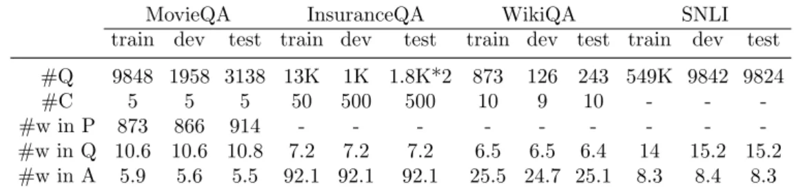
4.1 The example on the left is a machine comprehension problem from MovieQA, where the correct answer here is The Shire. The example on the right is an answer selection problem from InsuranceQA. . . 36 4.2 The statistics of different datasets. Q:question/hypothesis, C:candidate

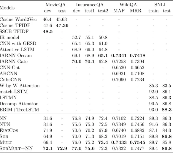
answers for each question, A:answer/hypothesis, P:plot, w:word (average). . . 44 4.3 Experiment Results . . . 45 4.4 Ablation Experiment Results. “no preprocess”: remove the

pre-processing layer by directly using word embeddingsQandA to replaceQandA in Eqn. 4.1; “no attention”: remove the atten-tion layer by using mean pooling ofQ to replace all the vectors of Hin Eqn. 5.2. . . 46

5.1 A paragraph from Wikipedia and three associated questions to-gether with their answers, taken from the SQuAD dataset. The tokens in bold in the paragraph are our predicted answers while the texts next to the questions are the ground truth answers. . . 54 5.2 Experiment Results on SQuAD and MSMARCO datasets. Here

“LSTM with Ans-Ptr” removes the attention mechanism in match-LSTM (mmatch-LSTM) by using the final state of the match-LSTM for the question to replace the weighted sum of all the states. Our best boundary model is the further tuned model and its ablation study is shown in Table 5.4. “en” refers to ensemble method. . 65 5.3 Statistical analysis on the development datasets. #w: number

of words on average; P: passage; Q: question; A: answer; raw: raw data from the development dataset; seq/bou: the answers generated by the sequence/boundary models with match-LSTM. 66

5.4 Ablation study for our best boundary model on the develop-ment datasets. Our best model is a further tuned boundary model by considering “bi-Ans-Ptr” which adds bi-directional an-swer pointer, “deep” which adds another two-layer bi-directional LSTMs between the match-LSTM and the Answer Pointer lay-ers, and “elem” which adds element-wise comparison ,(hp_i −

Hqα|_i) and (hp_i Hqα|_i), into Eqn 5.3. “-pre-LSTM” refers to removing the pre-processing layer. . . 66

6.1 An example passage and two related multi-choice questions. The ground-truth answers are in bold. . . 73 6.2 Experiment Results. ∗ means it’s significant to the models

ab-lating either the hierarchical aggregation or co-matching state. . 78

7.1 An open-domain QA training example. Q: question, A: answer, P: passages retrieved by an IR model and ordered by IR score. 84 7.2 Statistics of the datasets. #q represents the number of

ques-tions. For the training dataset, we ignore the questions without any answer in all the retrieved passages. In the special case that there’s only one answer for the question, during training, we combine the question with the answer as the query to improve IR recall. Otherwise we use only the question. #p represents the number of passages and 14.8 / 100 means there are 14.8 pas-sages containing the answer on average out of the 100 paspas-sages. We use top50 passages retrieved by the IR model for testing. . 94

7.3 Open-domain question answering results. SR: Single Reader; SR2: Simple Ranker-Reader; R3: Reinforced Ranker-Reader; WebQtn: WebQuestions. The results show the average of 5 runs, with standard error in the superscript. The CuratedTREC and WebQuestions models are initialized by training on SQuADOPEN

first. On the bottom, YodaQA [3] and DrQA-MTL [10] use additional resources (usage of KB for the former, and multiple training datasets for the latter), so are not a true apple-to-apple comparison to the other methods. EM: Exact Match. . . 95 7.4 Effects of rankers from SR2 and R3 (on Quasar-T test dataset).

Here we use the same single reader model (SR) as the reader, combined with two different rankers. The performance of the two runs of SR2 and R3 (that provide the rankers) is listed at bottom. . . 97 7.5 Potential improvement on QA performance by improving the

ranker. The performance is based on the Quasar-T test dataset.

The TOP-3/5 performance is used to evaluate the further

po-tential improvement by improving rankers (see the “Popo-tential Improvement” section). . . 97 7.6 An example of the answers extracted by the R3 and SR2

meth-ods, given the question. The words in bold are the extracted an-swers. The passages are ranked by the highest score (Ranker+Reader) of the answer span in each passage. . . 98 7.7 The performance of Rankers (recall of the top-k ranked

pas-sages) on the Quasar-T test dataset. This evaluation is simply based on whether the ground-truth appears in the TOP-N pas-sages. IR directly uses the ranking score from raw dataset. . . . 98

8.1 Statistics of the datasets. #q represents the number of ques-tions for training (not counting the quesques-tions that don’t have ground-truth answer in the corresponding passages for train-ing set), development, and testtrain-ing datasets. #p is the number of passages for each question. For TriviaQA, we split the raw documents into sentence level passages and select the top 100 passages based on the its overlaps with the corresponding ques-tion. #p(golden) means the number of passages that contain the ground-truth answer in average. #p(aggregated) is the number of passages we aggregated in average for top 10 candidate an-swers provided by RC model. . . 113 8.2 Experiment results on three open-domain QA test datasets:

Quasar-T, SearchQA and TriviaQA (open-domain setting). EM: Exact Match. Full Re-ranker is the combination of three differ-ent re-rankers. . . 115 8.3 The upper bound (recall) of the Top-K answer candidates

gen-erated by the baseline R3 _{system (on dev set), which indicates}

the potential of the coverage-based re-ranker. . . 117 8.4 Results of running coverage-based re-ranker on different number

of the top-K answer candidates on Quasar-T (dev set). . . 118 8.5 Results of running strength-based re-ranker (counting) on

dif-ferent number of top-K answer candidates on Quasar-T (dev set). . . 119 8.6 An example from Quasar-T dataset. The ground-truth answer is

”Sesame Street”. Q: question, A: answer, P: passages containing corresponding answer. . . 120

Chapter 1

Introduction

1.1

Overview

Question answering (QA) [62, 34, 61, 10, 40, 1, 5] is one of the most important applications in natural language processing. The task is to build machines that can answer questions expressed in human language using information and knowledge found in sources such as a single article, a corpus of documents, a knowledge base, or even an image or a video. Intelligently solving this prob-lem can not only help humans obtain useful information from huge amount of textual resources more efficiently, but also help develop intelligent machines such as conversational agents. Question answering has drawn much attention in recent years with the development of deep learning techniques. There’re multiple QA tasks in different settings, such as answer selection (AS) [73], machine reading comprehension (MRC) [61], knowledge base question answer-ing (KBQA) [5], visual question answeranswer-ing (VQA) [1], open-domain question answering (OQA) [10], etc.. All these tasks need to generate an answer for a given question, while the differences lie in the different context information given to answer the question. For example, the context information can be several candidate answers in the AS task, a question-related passage in MRC task, a knowledge base such as Freebase in the KBQA task, a question-related

Task : I. Answer Selection task

Context: (a) Yes, it be possible have auto insurance without own a vehicle. You will purchase what be call a name ...

(b)Insurance not be a tax or merely a legal obligation because auto insurance follow a car...

(c) You shall have auto insurance any time you own a car ...

Question: Can I have auto insurance without a car?

Answer: (a)

Task : II. Machine Reading Comprehension task

Context: In 1870, Tesla moved to Karlovac, to attend school at the Higher Real Gymnasium, where he was profoundly influenced by a math teacher Martin Sekuli´c. The classes were held in Ger-man, as it was a school within the Austro-Hungarian Military Frontier. Tesla was able to perform integral calculus in his head, which prompted his teachers to believe that he was cheating. He finished a four-year term in three years, graduating in 1873.

Question: Why did Tesla go to Karlovac?

Answer: attend school at the Higher Real Gymnasium

Task : III. Open-domain Question Answering task Context: wholeWikipedia or any Web page

Question: What is the largest island in the Philippines?

answer: Luzon

Table 1.1: Examples for three different question answering tasks.

figure in the VQA task, or any information from the webs in the OQA task. The most challenging is arguably the the open-domain question answering task where only a question is given and we can actually make use of any resource to answer it. It’s likely the final goal of question answering systems, which can answer anything using existing knowledge in the world. In this thesis, we will mainly focus on three tasks, namely Answer Selection, Machine Reading Com-prehension and Open-domain Question Answering, which rely only on context information in raw text, as shown in Table 1.1.

In earlier days, people focused more on the task of answer selection, which relies on a sequence matching model to identify which context sequence can answer the question, as the first example shown in Table 1.1. Actually, there’re also many other tasks relying on sequence matching model, such as paraphrase identification, natural language inference, etc.. Some classical methods [82]

train a matching model, like SVM, based on human crafted features, such as Rouge scores, BLEU scores, etc., to identify how well the sequence pairs can be matched. And the candidate sequence that can receive a higher matching score with the question would be predicted as the answer. However, these features, such as BLEU scores, are based on the exact N-gram match, and lack deep semantics (e.g., they fail to recognize that “dog” and “animal” are related.), lack consideration of context information (e.g. “dog” and hot “dog” are different), lack the relations between the matched phrases (e.g. “dog” can be entailed by “animal” and contradicted by “cat”). Later on, the sequences are represented by vectorized representations through neural networks, and the similarity between the representations is used to show how well the sequences are matched. Although with the help of some general neural frameworks, such as LSTM and CNN, the model achieved a good performance on answer selec-tion tasks, the sequence level representaselec-tions built by LSTM and CNN are still not powerful enough to represent all the semantic meanings of a sequence. We still need more interactive representations between sequences. In this thesis, we will propose a new textual sequence matching framework, which will build the phrase level matching representation between sequences through attention mechanism, and the aggregation of all the phrase level matching represen-tations will represent how well the sequences are matched. Our models are designed to overcome the shortcomings of previous works as discussed above, and the experiment results shown that our models can achieve state-of-the-art performance on multiple answer selection tasks. Besides the answer selection tasks, our sequence matching framework is also one of the key component in the solutions to many other question answering tasks.

One of the most well-studied question answering tasks in recent years is ma-chine reading comprehension. After I designed the aforementioned sequence matching model, a natural question is whether this model can be applied to ma-chine reading comprehension. Specifically, in mama-chine reading comprehension,

question related passage is given as context, and we can answer the question based on the information from the passage. The example in Table 1.1 is one setting of machine reading comprehension where we can directly extract the answer phrase from the context. Previous methods [61] on this task use human crafted feature based methods. They first extract all the noun and verb phrases from the passages by a parser, and then rank them with their corresponding contextual features. However, human crafted features are always not powerful enough to represent how the question and the context are matched in deep semantics. In this thesis, we propose the first neural network structure which can extract the answer in sequence for the question. Specifically, we first make use of our previously proposed sequence matching model to build the matching representation for every word in the passage, so that the matching representa-tions can reflect how well the contextual information of the corresponding word can match the question and also reflect the probability of the word to be the answer. Then we further add a pointer [79] layer to point out the positions of the words that can compose the answer based on the matching presentations. According to the experiment result, our model can achieve a much better per-formance than human crafted feature based methods. This kind of framework has also been widely adopted in other models [66, 97, 10] for the machine reading comprehension tasks, and also the tasks of open-domain QA.

Another well-studied question answering tasks that is more challenging than machine reading comprehension is open-domain question answering, and I further explore how my previous work can be applied in this problem setting. In this setting, there’s no specific context given any more. We can get the answer from any resource, while in this thesis, we mainly focus on making use of the raw text from Wikipedia to extract the answer. Previous work [10] on this task follows a pipeline work, “search and read”. Specifically, they first make use of information retrieval (IR) models based on tf-idf values to retrieve the question-related passages from Wikipedia, and then train a reading

Figure 1.1: An overview of the frameworks for different question answering tasks.

comprehension model on the retrieved passages through distant supervision. However, the limitation of distant supervision is that the model will treat all the passages that contain the answer as golden passages. For example, the question can be “Where’s Singapore Management University?”, and one IR retrieved passage can be “SMU is in Singapore”, while another passage can be “Multiple universities are in Singapore”. Although the ground-truth answer “Singapore” appears in both of the passages, the second passage is not closely related to the question. And it shouldn’t be used to train our reading comprehension model. In this way, we propose to use a neural ranker to select the passages for training the reading comprehension model (reader), and make use of reinforcement learning to jointly train ranker and reader. The experiment results show the effectiveness of our model on several open-domain QA datasets.

task-Figure 1.2: An overview of the major components in the thesis.

specific frameworks to solve the problem, they actually rely heavily on a good textual sequence matching model. As shown in Figure 1.1, we have a compar-ison of the frameworks to solve different tasks. The sequence matching model is to build a matching representation between two sequences, as shown in Fig-ure 1.1 (a). It can be directly applied to the answer selection task by matching every candidate with the question and have a comparison of the matching re-sults for ranking, as shown in Figure 1.1 (b). For the tasks of machine reading comprehension and open-domain question answering, the sequence matching model is always the bottom layer to build the matching representations be-tween question and the passages, as shown in Figure 1.1 (c) and (d). The differences lie on how the reasoning module is constructed to extract the an-swer based on the matching representations.

Overall, this thesis consists of three parts, as shown in Figure 1.2: (I) textual sequence matching model, and (II) the adaptation of the sequence matching model to machine reading comprehension and (III) the adaptation of the sequence matching model to open-domain question answering tasks. In Part I, we propose two general sequence matching models to solve the answer

selection and textual entailment tasks. In Part II, we propose two models to solve two types of machine reading comprehension tasks (MRC): answer span based and multi-choice based MRC. In Part III, we propose two models to handle noise and diversity issues in the IR retrieved passages from the task of open-domain question answering respectively.

1.2

Thesis Outline and Contributions

In Chapter 2, I will show the related works for the three major parts of this thesis. And then I’ll introduce more details of our models in the following chapters.

1.2.1

Textual Sequence Matching

In Chapter 3, I will first address the task of natural language inference, one of key tasks for solving question answering. In this task, we need to identify the relationship between a premise and a hypothesis. The relationship can be “entailment”, “contradiction” or “neutral”. To solve this problem, models with sequence matching are always applied. In previous work, LSTM based siamese neural networks and LSTM with attention mechanism have been ex-plored on this task. Unlike these models based on matching between the sequence-level representations, we propose a model named match-LSTM [86] which performs the matching in a word-by-word manner. In more details, we will first use LSTM to pre-process both sequences. Then every hidden state of these pre-processing LSTM will integrate not only the word information in the corresponding position but also its context information. Next, we further use these states to compute the attention weights. For each state in one sequence, we compute an attention vector which is the weighted sum of all the hidden states of the other sequence, and each pair of vectors (one hidden state and its attention vector) can represent the matched word pairs. And they will be

the inputs of another LSTM which aggregates all the matched word pairs in order. The final state of this LSTM will be used for the final classification. By making use of this model, we achieved state of the art performance on Stanford Natural Language Inference [7] dataset at the time our paper was published.. In Chapter 4, we further explore a more general and efficient compare-aggregate model [87] for sequence matching. For the compare-compare-aggregate model, we further research on the different word-level matching functions in the “com-pare” part, which is to build the representation between each word in one sequence and its corresponding attention vector, the weighted sum of all the hidden states of the other sequence. We start from applying the most complex function of Neural Tensor Networks to the simplest function of Euclidean Dis-tance to make the word level comparison across sequences. Then we further add a CNN layer to aggregate the comparison representations. To test the ef-fectiveness of different comparison functions, we further explore our model on another three answer selection datasets besides the natural language inference dataset. According to the experiment results, we find that the element-wise comparison function with the complexity in the middle works the best, and achieved state of the art on four different datasets.

1.2.2

Machine Reading Comprehension

In Chapter 5, I will focus on the task of answer-span based reading comprehen-sion, where a passage is given for each question and the ground-truth answer can be extracted from the given passage. To get the answer positions in the passage, we need to match the passage with question first to locate the poten-tial sub-sequence that could match the question. Then, another reasoning layer could be added to extract the exact answer span based on the previous match-ing representations. Based on this process, our model [88] uses match-LSTM to match the passage with the question, and further uses Pointer Network to

find the answer. The pointer network is the reasoning module shown in Fig-ure 1.1 (c), and it can point out which word in the given passage can be used to compose the final answer. And we propose two ways to find the answer: 1) word-by-word pointing until the end, so that all the pointed words will compose the answer sequence; 2) start and end positions pointing, and all the words between the start and end positions will compose the answer sequence. Based on the experiment results, we can clearly see that the second way for answer extraction is much better and achieved state of the art on SQuAD [61] and MSMARCO [57] datasets.

In Chapter 6, we try to solve another more challenging reading compre-hension task, the English examination from middle/high school. A question related passage is given for this task. Besides, several candidate answers are also given, and we can select the answer from the candidates. That is the ma-jor difference between previous answer span based reading comprehension and this task. For our model, instead of building representation between two types of sequence, either question matching passage (span-based reading compre-hension) or question matching candidate (answer selection), we need to build sequence matching representations for three types of sequences: passage, ques-tion, candidate answers. As the passage is the key component to explain how the ground-truth answer can entail the question, we propose a “co-matching” based model to match the passage with question and candidate answers in word-level at the same time, and make use of another hierarchical structure to integrate the “co-matching” representation. And our model achieved state of the art performance on the RACE dataset [46].

1.2.3

Open-Domain Question Answering

In Chapter 7, we present a novel open-domain QA system called Reinforced Ranker-Reader(R3_{) consisting of a ranking model (ranker) and a reading}

com-prehension model (reader). Our model is to extract the answer from IR re-trieved passages, but the problem is that we don’t know which passage can entail/answer the question. Even thought some passages containing the ground truth, they should not be used to train our reading comprehension model. In this way, we propose to use a neural ranker to select the passage for training the reader which can extract the exact answer phrase from the selected passage. As the selecting action by ranker is non-differentiable, in order to jointly train the ranker and reader, we make use of the method REINFORCE [96]. And our experiments show that our Reinforced Ranker-Reader can outperform the baseline which ensembles the ranker and reader trained separately under dis-tance supervision. Moreover, our model achieved state-of-the-art performance on three open-domain QA datasets.

In Chapter 8, by observing that some questions require a combination of evidence from across different sources to answer correctly, we propose two methods to address this issue. Suppose the passages that contain the same candidate answer are strongly related, and our goal is to make use these pas-sages for evidence aggregation to answer questions. The easiest way to get the candidate answers is just using the Reinforced Ranker-Reader (R3_{) in}

chap-ter 7, and we could re-rank these candidates by combining the evidence from the passages containing the corresponding candidate answer. We propose two methods, namely, strength-based re-ranking and coverage-based re-ranking, to solve the problem. For strength-based re-ranking, the hypothesis is that the more evidence that can support the candidate, the more likely it would be the ground-truth answer. Here, we treat the passage as supporting evidence for one candidate if the pre-trained model Reinforced Ranker-Reader (R3_{) can}

generate the candidate. Then we can rank the candidates by either counting the number of supporting evidence or accumulating the probabilities provided by (R3). For the coverage-based re-ranking, we will concatenate all the pas-sages containing one candidate answer together and treat it as a new sequence,

so that the new sequence will contain all the evidence related to the candidate answer. Then we will directly match the new sequence with the question to check whether the aggregated evidence from different passages can entail the question. The model here is to use textual sequence matching for ranking. Ac-cording to our experiment results, both of our models can outperform previous best results on three different open-domain QA datasets.

Overall, this thesis will cover my published papers as the first author as follows:

• Learning Natural Language Inference with LSTM [86], InProceedings of the Conference on the North American Chapter of the Association for Computational Linguistics (NAACL), 2016.

• A Compare-aggregate Model for Matching Text Sequences [87], In Pro-ceedings of the International Conference on Learning Representations (ICLR), 2017.

• Machine Comprehension Using Match-LSTM and Answer Pointer [88], In

Proceedings of the International Conference on Learning Representations (ICLR), 2017.

• A Co-Matching Model for Multi-choice Reading Comprehension [89], In

Proceedings of the Conference on Association for Computational Linguis-tics (ACL), 2018.

• R3_{: Reinforced Reader-Ranker for Open-Domain Question}

Answer-ing [90], In Proceedings of AAAI Conference on Artificial Intelligence (AAAI), 2018.

• Evidence Aggregation for Answer Re-Ranking in Open-Domain Ques-tion Answering [91], In Proceedings of the International Conference on Learning Representations (ICLR), 2018

Chapter 2

Related work

In this chapter, I’ll discuss the related work on solving different question an-swering tasks, especially machine reading comprehension and open-domain question answering, with textual sequence matching models.

2.1

Textual Sequence Matching

Many answer selection tasks are based on the the textual sequence matching model. We will review related works in three types of general structures for matching sequences.

Siamense network: These kinds of models use the same structure, such as

RNN or CNN, to build the representations for the sequences separately. Then cosine similarity [26, 99], element-wise operation [71, 55] or neural network-based combination [7] are used for sequence matching.

Attentive network: Soft-attention mechanism [2, 49] has been widely

used for sequence matching in machine comprehension [34], text entailment [64] and question answering [72]. Instead of using the final state of RNN to rep-resent a sequence, these studies use weighted sum of all the states for the sequence representation.

the word level matching [88, 58, 33, 76, 83]. Our works are under this frame-work. But our structures are different from previous models and our model can be applied on different tasks. Besides, we analyzed different word-level comparison functions separately.

2.2

Machine Reading Comprehension

Machine reading comprehension of text has gained much attention in recent years, and increasingly researchers are building data-driven, end-to-end neural network models for the task. We will first review the recently released datasets and then some end-to-end models on this task.

2.2.1

Datasets

A number of datasets for studying machine reading comprehension were cre-ated in Cloze style by removing a single token from a sentence in the original corpus, and the task is to predict the missing word. For example, [34] created questions in Cloze style from CNN and Daily Mail highlights. [36] created the Children’s Book Test dataset, which is based on children’s stories. [19] released two similar datasets in Chinese, the People Daily dataset and the Children’s Fairy Tale dataset.

Instead of creating questions in Cloze style, a number of other datasets rely on human annotators to create real questions. [62] created the well-known MCTest dataset and [75] created the MovieQA dataset. In these datasets, can-didate answers are provided for each question. Similar to these two datasets, the SQuAD dataset [61] was also created by human annotators. Different from the previous two, however, the SQuAD dataset does not provide candidate an-swers, and thus all possible subsequences from the given passage have to be considered as candidate answers.

for machine comprehension, such as WikiReading dataset [35] and bAbI dataset [94], but they are quite different from the datasets above in nature.

2.2.2

End-to-end Neural Network Models for Machine

Comprehension

There have been a number of studies proposing end-to-end neural network models for machine comprehension. A common approach is to use recurrent neural networks (RNNs) to process the given text and the question in order to predict or generate the answers [34]. Attention mechanism is also widely used on top of RNNs in order to match the question with the given passage [34, 9]. Given that answers often come from the given passage, Pointer Network has been adopted in a few studies in order to copy tokens from the given passage as answers [41, 78]. Compared with existing work, we use match-LSTM to match a question and a given passage, and we use Pointer Network in a different way such that we can generate answers that contain multiple tokens from the given passage.

Memory Networks [95] have also been applied to machine comprehen-sion [70, 44, 36], but its scalability when applied to a large dataset is still an issue. In this thesis, we did not consider memory networks for the SQuAD/MSMARCO datasets.

2.3

Open-domain Question Answering

Open domain question answering dates back to as early as [31] and was pop-ularized with TREC-8 [80]. The task is to answer a question by exploiting resources such as documents [80], webpages [45, 13] or structured knowledge bases [5, 6, 103]. An early consensus since TREC-8 has produced an approach with three major components: question analysis, document retrieval and

rank-ing, and answer extraction. Although question analysis is relatively mature, answer extraction and document ranking still represent significant challenges. Very recently, IR plus machine reading comprehension (SR-QA) showed promise for open-domain QA, especially after datasets created specifically for the multiple-passage RC setting [57, 10, 40, 24, 23]. These datasets deal with the end-to-end open-domain QA setting, where only question-answer pairs provide supervision. Similarly to previous work on open-domain QA, existing deep learning based solutions to the above datasets also rely on a document retrieval module to retrieve a list of passages for RC models to extract answers. Therefore, these approaches suffer from the limitation that the passage ranking scores are determined by n-gram matching (with tf-idf weighting), which is not ideal for QA.

Our ranker module in R3 could help to alleviate the above problem, and RL is a natural fit to jointly train the ranker and reader since the passages do not have ground-truth labels. Our work is related to the idea of soft or hard attentions (usually with reinforcement learning) for hierarchical or coarse-to-fine decision sequences making in NLP, where the attentions themselves are latent variables. For example, [47] propose to first extract informative text fragments then feed them to text classification and question retrieval models. [15] and [16] proposed coarse-to-fine frameworks with an additional sentence selection step before the original word-level prediction for text summarization and reading comprehension, respectively. To the best of our knowledge, we are the first apply this kind of framework to the open-domain question answering. From the method-perspective, our work is most close to [16]’s work in terms of the usage of REINFORCE. Our main aim is to deal with the lack of annotation in the passage selection step, which is a necessary intermediate step in open-domain QA. In comparison, [16] has as its main aim to speed up the RC model in the single passage setting. From the motivation-perspective, we are similar to [56]’s work. Both work aim to find passages easy and suitable

Part I

General Textual Sequence

Matching Models

Chapter 3

Learning Natural Language

Inference with Match-LSTM

In this chapter, I will introduce “match-LSTM”, which is based on sequence-to-sequence word-level matching, for the task of natural language inference.

3.1

Introduction

Natural language inference (NLI) is the problem of determining whether from a premise sentence P one can infer another hypothesis sentence H [50]. NLI is a fundamentally important problem that has applications in many tasks including question answering, semantic search and automatic text summariza-tion. There has been much interest in NLI in the past decade, especially sur-rounding the PASCAL Recognizing Textual Entailment (RTE) Challenge [20]. Existing solutions to NLI range from shallow approaches based on lexical sim-ilarities [29] to advanced methods that consider syntax [53], perform explicit sentence alignment [51] or use formal logic [17].

Recently, [7] released the Stanford Natural Language Inference (SNLI) cor-pus for the purpose of encouraging more learning-centered approaches to NLI. This corpus contains around 570K sentence pairs with three labels: entailment,

contradiction andneutral. The size of the corpus makes it now feasible to train deep neural network models, which typically require a large amount of training data. [7] tested a straightforward architecture of deep neural networks for NLI. In their architecture, the premise and the hypothesis are each represented by a sentence embedding vector. The two vectors are then fed into a multi-layer neural network to train a classifier. [7] achieved an accuracy of 77.6% when long short-term memory (LSTM) networks were used to obtain the sentence embeddings.

A more recent work by [65] improved the performance by applying a neu-ral attention model. While their basic architecture is still based on sentence embeddings for the premise and the hypothesis, a key difference is that the embedding of the premise takes into consideration the alignment between the premise and the hypothesis. This so-called attention-weighted representation of the premise was shown to help push the accuracy to 83.5% on the SNLI corpus.

A limitation of the aforementioned two models is that they reduce both the premise and the hypothesis to a single embedding vector before matching them; i.e., in the end, they use two embedding vectors to perform sentence-level matching. However, not all word or phrase-sentence-level matching results are equally important. For example, the matching between stop words in the two sentences is not likely to contribute much to the final prediction. Also, for a hypothesis to contradict a premise, a single word or phrase-level mismatch (e.g., a mismatch of the subjects of the two sentences) may be sufficient and other matching results are less important, but this intuition is hard to be captured if we directly match two sentence embeddings.

In this chapter, we propose a new LSTM-based architecture for learning natural language inference. Different from previous models, our prediction is not based on whole sentence embeddings of the premise and the hypothesis. Instead, we use an LSTM to performword-by-word matching of the hypothesis

with the premise. Our LSTM sequentially processes the hypothesis, and at each position, it tries to match the current word in the hypothesis with an attention-weighted representation of the premise. Matching results that are critical for the final prediction will be “remembered” by the LSTM while less important matching results will be “forgotten.” We refer to this architecture a match-LSTM, ormLSTM for short.

Experiments show that our mLSTM model achieves an accuracy of 86.1% on the SNLI corpus, outperforming the state of the art. Furthermore, through further analyses of the learned parameters, we show that themLSTM architec-ture can indeed pick up the more important word-level matching results that need to be remembered for the final prediction. In particular, we observe that good word-level matching results are generally “forgotten” but important mis-matches, which often indicate a contradiction or a neutral relationship, tend to be “remembered.”

Our code is available online1_.

3.2

Model

In this section, we first review the word-by-word attention model by [65], which is their best performing model. Then we present ourmLSTM architecture for natural language inference.

3.2.1

Neural Attention Model

For the natural language inference task, we have two sentences Xs ₌

(xs

1,xs2, . . . ,xsM) and Xt = (x1t,xt2, . . . ,xtN), where Xs is the premise and Xt

is the hypothesis. Here each x is an embedding vector of the corresponding word. The goal is to predict a label y that indicates the relationship between

Xs and Xt. In this chapter, we assume y is one of entailment, contradiction

and neutral.

[65] first used two LSTMs to process the premise and the hypothesis, re-spectively, but initialized the second LSTM (for the hypothesis) with the last cell state of the first LSTM (for the premise). Let us use hs

j and htk to denote

the resulting hidden states corresponding toxs_j andxt_k, respectively. The main idea of the word-by-word attention model by [65] is to introduce a series of attention-weighted combinations of the hidden states of the premise, where each combination is for a particular word in the hypothesis. Let us use ak to

denote such an attention vector for word xt

k in the hypothesis. Specifically,ak

is defined as follows2_: ak = M X j=1 αkjhsj, (3.1)

where αkj is an attention weight that encodes the degree to which xtk in the

hypothesis is aligned with xs_j in the premise. The attention weight αkj is

generated in the following way:

αkj = exp(ekj) P j0exp(e_kj0), (3.2) where ekj =we·tanh(Wshsj+Wthtk+Wahak−1). (3.3)

Here · is the dot-product between two vectors, the vector we _∈

Rd and all

matricesW* _∈

Rd×dcontain weights to be learned, andhak−1is another hidden

state which we will explain below.

2_{We present the word-by-word attention model by [65] in a different way but the}

under-lying model is the same. Our ha

k is theirrt, our Hs (all of hsj) is their Y, our htk is their

ht, and our αk is their αt. Our presentation is close to the one by [2], with our attention vectorsacorresponding to the context vectorscin their paper.

The attention-weighted premise ak essentially tries to model the relevant

parts in the premise with respect to xt

k, i.e., the kth word in the hypothesis.

[65] further built an RNN model over{ak}Nk=1 by defining the following hidden

states:

ha_k = ak+ tanh(Vahak−1), (3.4)

where Va _∈

Rd×d is a weight matrix to be learned. We can see that the last

ha

N aggregates all the previous ak and can be seen as an attention-weighted

representation of the whole premise. [65] then used this ha

N, which represents

the whole premise, together with ht

N, which can be approximately regarded as

an aggregated representation of the hypothesis3_{, to predict the labely.}

3.2.2

Our Model

Although the neural attention model by [65] achieved better results than [7], we see two limitations. First, the model still uses a single vector representation of the premise, namely ha_N, to match the entire hypothesis. We speculate that if we instead use each of the attention-weighted representations of the premise for matching, i.e., use ak at position k to match the hidden state htk

of the hypothesis while we go through the hypothesis, we could achieve better matching results. This can be done using an RNN which at each position takes in both ak and htk as its input and determines how well the overall matching

of the two sentences is up to the current position. In the end the RNN will produce a single vector representing the matching of the two entire sentences. The second limitation is that the model by [65] does not explicitly allow us to place more emphasis on the more important matching results between

3_{Strictly speaking, in the model by [65],h}t

N encodes both the premise and the hypothesis because the two sentences are chained. Butht_N places a higher emphasis on the hypothesis given the nature of RNNs.

Figure 3.1: The top figure depicts the model by Rockt¨aschel et al. (2016) and the bottom figure depicts our model. Here Hs represents all the hidden states

hs

j. Note that in the top model each hak represents a weighted version of the

premise only, while in our model, each hm

k represents the matching between

the premise and the hypothesis up to positionk.

the premise and the hypothesis and down-weight the less critical ones. For example, matching of stop words is presumably less important than matching of content words. Also, some matching results may be particularly critical for making the final prediction and thus should be remembered. For example, consider the premise “A dog jumping for a Frisbee in the snow.” and the hypothesis “A cat washes his face and whiskers with his front paw.” When we sequentially process the hypothesis, once we see that the subject of the hypothesis cat does not match the subject of the premise dog, we have a high probability to believe that there is a contradiction. So this mismatch should be remembered.

Based on the two observations above, we propose to use an LSTM to se-quentially match the two sentences. At each position the LSTM takes in both

ak and htk as its input. Figure 3.1 gives an overview of our model in contrast

to the model by [65].

Specifically, our model works as follows. First, similar to [65], we process the premise and the hypothesis using two LSTMs, but we do not feed the last

cell state of the premise to the LSTM of the hypothesis. This is because we do not need the LSTM for the hypothesis to encode any knowledge about the premise but we will match the premise with the hypothesis using the hidden states of the two LSTMs. Again, we use hs

j and htk to represent these hidden

states.

Next, we generate the attention vectorsaksimilarly to Eqn (3.1). However,

Eqn (3.3) will be replaced by the following equation:

ekj =we·tanh(Wshsj+Wthtk+Wmhmk−1). (3.5)

The only difference here is that we use a hidden state hm instead of ha, and the way we definehm is very different from the definition of ha.

Our hm

k is the hidden state at position k generated from our mLSTM.

This LSTM models the matching between the premise and the hypothesis. Important matching results will be “remembered” by the LSTM while non-essential ones will be “forgotten.” We use the concatenation of ak, which is

the attention-weighted version of the premise for thekthword in the hypothesis, and ht_k, the hidden state for the kth word itself, as input to the mLSTM.

Specifically, let us define

mk =    ak ht_k   . (3.6)

im_k = σ(Wmimk+Vmihmk−1+bmi), f_km = σ(Wmfmk+Vmfhmk−1+bmf), om_k = σ(Wmomk+Vmohmk−1+bmo), cm_k = f_kmcm_k−1+imk tanh(Wmcmk+Vmchmk−1 +bmc), hm_k = om_k tanh(cm_k). (3.7)

With this mLSTM, finally we use only hm_N, the last hidden state, to predict the label y.

3.2.3

Implementation Details

Besides the difference of the LSTM architecture, we also introduce a few other changes from the model by [65]. First, we insert a special word NULL to the premise, and we allow words in the hypothesis to be aligned with this NULL. This is inspired by common practice in machine translation. Specifically, we introduce a vector hs

0, which is fixed to be a vector of 0s of dimension d. This hs

0 represents NULL and is used with other hsj to derive the attention vectors {ak}Nk=1.

Second, we use word embeddings trained from GloVe [59] instead of word2vec vectors. The main reason is that GloVe covers more words in the SNLI corpus than word2vec4_.

Third, for words which do not have pre-trained word embeddings, we take the average of the embeddings of all the words (in GloVe) surrounding the unseen word within a window size of 9 (4 on the left and 4 on the right) as an approximation of the embedding of this unseen word. Then we do not update

4_{The SNLI corpus contains 37K unique tokens. Around 12.1K of them cannot be found}

Model d |θ|_W+M |θ|_M Train Dev Test

LSTM [[7]] 100 10M 221K 84.4 - 77.6

Classifier [[7]] - - - 99.7 - 78.2

LSTM shared [[65]] 159 3.9M 252K 84.4 83.0 81.4 Word-by-word attention [[65]] 100 3.9M 252K 85.3 83.7 83.5 Word-by-word attention (our implementation) 150 340K 340K 85.5 83.3 82.6

mLSTM 150 544K 544K 91.0 86.2 85.7

mLSTM with bi-LSTM sentence modeling 150 1.4M 1.4M 91.3 86.6 86.0

mLSTM 300 1.9M 1.9M 92.0 86.9 86.1

mLSTM with word embedding 300 1.3M 1.3M 88.6 85.4 85.3

Table 3.1: Experiment results in terms of accuracy. d is the dimension of the hidden states. |θ|W+Mis the total number of parameters and|θ|Mis the number

of parameters excluding the word embeddings. Note that the five models in the last section were implemented by us while the other results were taken directly from previous papers. Note also that for the five models in the last section, we do not update word embeddings so |θ|W+M is the same as |θ|M.

The three columns on the right are the accuracies of the trained models on the training data, the development data and the test data, respectively.

any word embedding when learning our model. Although this is a very crude approximation, it reduces the number of parameters we need to update, and as it turns out, we can still achieve better performance than [65].

3.3

Experiments

3.3.1

Experiment Settings

Data: We use the SNLI corpus to test the effectiveness of our model. The

original data set contains 570,152 sentence pairs, each labeled with one of the following relationships: entailment, contradiction, neutral and –, where

– indicates a lack of consensus from the human annotators. We discard the sentence pairs labeled with–and keep the remaining ones for our experiments. In the end, we have 549,367 pairs for training, 9,842 pairs for development and 9,824 pairs for testing. This follows the same data partition used by [7] in their experiments. We perform three-class classification and use accuracy as

our evaluation metric.

Parameters: We use the Adam method [43] with hyperparameters β1 set to

0.9 and β2 set to 0.999 for optimization. The initial learning rate is set to be

0.001 with a decay ratio of 0.95 for each iteration. The batch size is set to be 30. We experiment with d = 150 andd = 300 where d is the dimension of all the hidden states.

Methods for comparison: We mainly want to compare our model with the

word-by-word attention model by [65] because this model achieved the state-of-the-art performance on the SNLI corpus. To ensure fair comparison, besides comparing with the accuracy reported by [65], we also re-implemented their model and report the performance of our implementation. We also consider a few variations of our model. Specifically, the following models are implemented and tested in our experiments:

• Word-by-word attention (d = 150): This is our implementation of the word-by-word attention model by [65], where we set the dimension of the hidden states to 150. The differences between our implementation and the original implementation by [65] are the following: (1) We also add a

NULL token to the premise for matching. (2) We do not feed the last cell state of the LSTM for the premise to the LSTM for the hypothesis, to keep it consistent with the implementation of our model. (3) For word representation, we also use the GloVe word embeddings and we do not update the word embeddings. For unseen words, we adopt the same strategy as described in Section 3.2.3.

• mLSTM (d= 150): This is ourmLSTM model with d set to 150.

• mLSTM with bi-LSTM sentence modeling (d = 150): This is the same as the model above except that when we derive the hidden states hs_j and

ht_k of the two sentences, we use bi-LSTMs [30] instead of LSTMs. We implement this model to see whether bi-LSTMs allow us to better align the sentences.

ground truth prediction N E C

N 2628 286 255

E 340 3005 159

C 250 77 2823

Table 3.2: The confusion matrix of the results by mLSTM with d = 300. N,

E and C correspond to neutral, entailment and contradiction, respectively.

ID sentence label

Premise A dog jumping for a Frisbee in the snow. Example 1 An animal is outside in the cold weather,

playing with a plastic toy.

entailment Hypothesis Example 2 A cat washed his face and whiskers with

his front paw.

contradiction Example 3 A pet is enjoying a game of fetch with his

owner.

neutral

Table 3.3: Three examples of sentence pairs with different relationship labels. The second hypothesis is a contradiction because it mentions a completely different event. The third hypothesis is neutral to the premise because the phrase “with his owner” cannot be inferred from the premise.

• mLSTM (d= 300): This is ourmLSTM model with d set to 300.

• mLSTM with word embedding (d= 300): This is the same as the model above except that we directly use the word embedding vectorsxs

j and xtk

instead of the hidden states hs

j and htk in our model. In this case, each

attention vector ak is a weighted sum of {xsj}Mj=1. We experiment with

this setting because we hypothesize that the effectiveness of our model is largely related to themLSTM architecture rather than the use of LSTMs to process the original sentences.

3.3.2

Main Results

Table 3.1 compares the performance of the various models we tested together with some previously reported results.

We have the following observations: (1) First of all, we can see that when we set d to 300, our model achieves an accuracy of 86.1% on the test data, which to the best of our knowledge is the highest on this data set. (2) If we

compare our mLSTM model with our implementation of the word-by-word attention model by [65] under the same setting with d= 150, we can see that our performance on the test data (85.7%) is higher than that of their model (82.6%). We also tested statistical significance and found the improvement to be statistically significant at the 0.001 level. (3) The performance of mLSTM with bi-LSTM sentence modeling compared with the model with standard LSTM sentence modeling when d is set to 150 shows that using bi-LSTM to process the original sentences helps (86.0% vs. 85.7% on the test data), but the difference is small and the complexity of bi-LSTM is much higher than LSTM. Therefore when we increased d to 300 we did not experiment with bi-LSTM sentence modeling. (4) Interestingly, when we experimented with the mLSTM model using the pre-trained word embeddings instead of LSTM-generated hidden states as initial representations of the premise and the hypothesis, we were able to achieve an accuracy of 85.3% on the test data, which is still better than previously reported state of the art. This suggests that the mLSTM architecture coupled with the attention model works well, regardless of whether or not we use LSTM to process the original sentences.

Because the NLI task is a three-way classification problem, to better un-derstand the errors, we also show the confusion matrix of the results obtained by our mLSTM model with d = 300 in Table 3.2. We can see that there is more confusion between neutral andentailment and between neutral and con-tradiction than betweenentailment andcontradiction. This shows thatneutral

is relatively hard to capture.

3.3.3

Further Analyses

To obtain a better understanding of how our proposed model actually performs the matching between a premise and a hypothesis, we further conduct the fol-lowing analyses. First, we look at the learned word-by-word alignment weights

Figure 3.2: The alignment weights and the gate vectors of the three examples.

αkj to check whether the soft alignment makes sense. This is the same as what

was done by [65]. We then look at the values of the various gate vectors of the

mLSTM. By looking at these values, we aim to check (1) whether the model is able to differentiate between more important and less important word-level matching results, and (2) whether the model forgets certain matching results and remembers certain other ones.

To conduct the analyses, we choose three examples and display the various learned parameter values. These three sentence pairs share the same premise

but have different hypotheses and different relationship labels. They are given in Table 3.3. The values of the alignment weights and the gate vectors are plotted in Figure 3.2.

Besides using the three examples, we will also give some overall statistics of the parameter values to confirm our observations with the three examples.

Word Alignment

First, let us look at the top-most plots of Figure 3.2. These plots show the alignment weightsαkj between the hypothesis and the premise, where a darker

color corresponds to a larger value ofαkj. Recall thatαkj is the degree to which

thekth_{word in the hypothesis is aligned with thej}th _{word in the premise. Also}

recall that the weights αkj are configured such that for the same k all theαkj

add up to 1. This means the weights in the same row in these plots add up to 1. From the three plots we can see that the alignment weights generally make sense. For example, in Example 1, “animal” is strongly aligned with “dog” and “toy” aligned with “Frisbee.” The phrase “cold weather” is aligned with “snow.” In Example 3, we also see that “pet” is strongly aligned with “dog” and “game” aligned with “Frisbee.”

In Example 2, “cat” is strongly aligned with “dog” and “washes” is aligned with “jumping.” It may appear that these matching results are wrong. How-ever, “dog” is likely the best match for “cat” among all the words in the premise, and as we will show later, this match between “cat” and “dog” is actually a strong indication of a contradiction between the two sentences. The same explanation applies to the match between “washes” and “jumping.”

We also observe that some words are aligned with the NULL token we inserted. For example, the word “is” in the hypothesis in Example 1 does not correspond to any word in the premise and is therefore aligned with NULL. The words “face” and “whiskers” in Example 2 and “owner” in Example 3 are

also aligned with NULL. Intuitively, if some important content words in the hypothesis are aligned with NULL, it is more likely that the relationship label is either contradiction or neutral.

Values of Gate Vectors

Next, let us look at the values of the learned gate vectors of our mLSTM for the three examples. We show these values under the setting where d is set to 150. Each row of these plots corresponds to one of the 150 dimensions. Again, a darker color indicates a higher value.

An input gate controls whether the input at the current position should be used in deriving the final hidden state of the current position. From the three plots of the input gates, we can observe that generally for stop words such as prepositions and articles the input gates have lower values, suggesting that the matching of these words is less important. On the other hand, content words such as nouns and verbs tend to have higher values of the input gates, which also makes sense because these words are generally more important for determining the final relationship label.

To further verify the observation above, we compute the average input gate values for stop words and the other content words. We find that the former has an average value of 0.287 with a standard deviation of 0.084 while the latter has an average value of 0.347 with a standard deviation of 0.116. This shows that indeed generally stop words have lower input gate values. Interestingly, we also find that some stop words may have higher input gate values if they are critical for the classification task. For example, the negation word “not” has an average input gate value of 0.444 with a standard deviation of 0.104.

Overall, the values of the input gates confirm that themLSTM helps differ-entiate the more important word-level matching results from the less important ones.

Next, let us look at the forget gates. Recall that a forget gate controls the importance of the previous cell state in deriving the final hidden state of the current position. Higher values of a forget gate indicate that we need to remember the previous cell state and pass it on whereas lower values indicate that we should probably forget the previous cell. From the three plots of the forget gates, we can see that overall the colors are the lightest for Example 1, which is anentailment. This suggests that when the hypothesis is an entailment of the premise, the mLSTM tends to forget the previous matching results. On the other