VISPARK: GPU-ACCELERATED DISTRIBUTED VISUAL
COMPUTING USING SPARK
∗WOOHYUK CHOI†, SUMIN HONG†, AND WON-KI JEONG†
Abstract. With the growing need of big-data processing in diverse application domains, MapReduce (e.g., Hadoop) has become one of the standard computing paradigms for large-scale computing on a cluster system. Despite its popularity, the current MapReduce framework suffers from inflexibility and inefficiency inherent to its programming model and system architecture. In or-der to address these problems, we proposeVispark, a novel extension ofSparkfor GPU-accelerated MapReduce processing on array-based scientific computing and image processing tasks. Vispark provides an easy-to-use, Python-like high-level language syntax and a novel data abstraction for MapReduce programming on a GPU cluster system. Vispark introduces a programming abstraction for accessing neighbor data in the mapper function, which greatly simplifies many image processing tasks using MapReduce by reducing memory footprints and bypassing the reduce stage. Vispark provides socket-based halo communication that synchronizes between data partitions transparently from the users, which is necessary for many scientific computing problems in distributed systems. Vispark also provides domain-specific functions and language supports specifically designed for high-performance computing and image processing applications. We demonstrate the high-performance of our prototype system on several visual computing tasks, such as image processing, volume rendering, K-means clustering, and heat transfer simulation.
Key words. MapReduce, GPU, distributed computing, visualization, domain-specific language AMS subject classifications. 65Y05, 68Q85
DOI. 10.1137/15M1026407
1. Introduction.
With advent of advances in data acquisition and network
technology,
big data
has become one of the hottest buzzwords these days. Big data
commonly refers to datasets of sizes beyond the capability of conventional data
pro-cessing workflow, ranging from a few terabytes to petabytes. In his technical
re-port [17], Laney defined big data using the “3Vs” (high volume, high velocity, and
high variety). According to this definition, not only the sheer size of the data but
also its acquisition speed and diversity in data type represent the characteristics of
big data. Applications of big data can be found in diverse fields, such as Internet
and media service, government, retail business, and science and technology. For
ex-ample, Facebook processes around 2.5 billion pieces of content and 500 terabytes of
data daily [21]. Multibeam electron microscopes collect roughly 2.5 terabytes of brain
images per hour in connectome research [16]. The Large Hadron Collider at CERN
continuously generates nearly 600 million collisions per second, which makes the data
rate higher than 150 million petabytes per year [6]. Such an extreme scale of data size
cannot be properly handled by a standard server-level computer using conventional
∗Received by the editors June 30, 2015; accepted for publication (in revised form) August 3, 2016; published electronically October 27, 2016.
http://www.siam.org/journals/sisc/38-5/M102640.html
Funding:This work was partially supported by an Institute for Information & Communications Technology Promotion (IITP) grant funded by the Korea government (MSIP) (R0190-16-2012, High Performance Big Data Analytics Platform Performance Acceleration Technologies Development) and the Basic Science Research Program through the National Research Foundation of Korea (NRF) funded by the Ministry of Education (NRF-2014R1A1A2058773).
†School of Electrical and Computer Engineering, Ulsan National Institute of Science and Tech-nology, Ulsan, Republic of Korea ([email protected], [email protected], [email protected]).
data analysis software. Therefore, in the era of big data, we need a paradigm shift in
computing and programming models.
One of the most popular big data processing models is
MapReduce
[11], and its
open-source implementation is
Hadoop
[2]. In this programming model, the task is
decomposed into two user-programmable stages—the
map
stage processes the input
data and generates key-value pairs, and the
reduce
stage processes a group of values for
the same key. There is a nonprogrammable sorting stage between the
map
and
reduce
stages, which arranges key-value data according to the order of keys. Hadoop provides
a simplified programming abstraction so that the user needs to implement only the
map
and
reduce
functions (i.e., the mapper and the reducer) without considering data
communication and task decomposition for large-scale distributed parallel processing.
The Hadoop system can run on a cluster of low-cost commodity PCs and provides a
software fault tolerance mechanism for reliable processing. Due to its simplicity and
reliability, Hadoop has become a de facto standard for big data processing in cluster
and cloud environments.
Despite its popularity, the Hadoop system also suffers from several drawbacks.
First, its programming model is too restrictive for certain types of computing tasks.
The main assumption of the MapReduce model is that the data are provided as a
list of key-value pairs, and there is no dependency between data values so that the
data can be easily decomposed into chunks and processed independently. However,
in many scientific computing and image processing problems, data are defined on
a regular grid, i.e., arrays, and the neighbor data are necessary for computation,
which makes the MapReduce system difficult to apply. The common approach is to
generate multiple copies of the input data in the mapper so that the reducer can
collect all the necessary neighbor data, which is unnecessarily inefficient in terms of
memory footprint. This inefficiency comes from the restriction of the MapReduce
programming model, where the mapper is designed to be executed on each data
element independently and neighbor data access is prohibited. Second, Hadoop is
not a performance-optimized system—data communication relies on a slow disk I/O,
and the runtime system is written in Java. Hadoop is designed to favor large-scale
distributed batch processing, but unlike conventional large-scale high-performance
computing (i.e., supercomputing), low-level performance optimization has not been an
important part of the system architecture. A recent study [3] shows that the scale-up
Hadoop performs better than the scale-out Hadoop, which confirms that there is still
much room for performance improvement in the current Hadoop/MapReduce system.
One of the notable recent MapReduce systems is Spark [26], which introduces
in-memory cache and streaming to improve the performance of the conventional Hadoop
system by reducing expensive disk I/O and reusing data in memory.
To address the limitation of the current Hadoop system, we propose
Vispark
, an
extension of the Spark MapReduce framework for high-performance visual computing
on a GPU-based cluster system. Vispark is a combination of a high-level
MapRe-duce programming language and its runtime system, and it is specifically designed to
overcome the problems of Hadoop by providing a simple programming model and
ab-straction to scale-up the system and leverage the state-of-the-art, high-performance
computing technology. Vispark’s language syntax is inspired by Vivaldi [10], a
domain-specific language for visualization that uses Python syntax and high-level abstractions
for volume rendering and computing. Without the knowledge of GPU-specific APIs
such as NVIDA CUDA, and OpenCL, the user can write a Python-like mapper code
using Vispark language, and the Vispark translator and runtime system will
automat-ically execute the code on the target GPU architecture. Vispark also provides a new
abstract data type, the
Vispark resilient distributed dataset (VRDD)
, to manage GPU
data in Spark, and synchronization between the CPU and the GPU is automatically
done via lazy evaluation of the Spark system. Another novel feature of Vispark is that
it provides a simple MapReduce programming abstraction,
Iterator
, and automatic
halo synchronization using socket communication, to access local data without explicit
data management by the user. Since the iterator will allow the mapper to access local
data, many scientific computing tasks using array data, such as stencil computations
on two-dimensional (2D) and 3D rectilinear grids, can be easily implemented in the
mapper stage. By doing that, the performance bottleneck of the disk-based shuffle
stage can be effectively avoided. We believe Vispark is a novel blending of a
domain-specific language and a MapReduce framework that unlocks the restrictions of the
conventional Hadoop and will eventually enhance the usability and performance of
the MapReduce system.
2. Related work.
MapReduce framework.
The concept of MapReduce, originally proposed by
Google [11], is considered a standard parallel computing framework for large-scale
un-structured data processing. In MapReduce, designing two stages of processing, such
as
map
and
reduce
, is left to the users, while the system deals with the rest of the
processing details, such as communication, scheduling, and data splitting. Hadoop [2]
is an open-source implementation of the MapReduce concept, and its ecosystem
pro-vides a wide variety of software stacks, such as the Hadoop Distributed File System
(HDFS), Yarn, and others. Recently, Spark [27] has evolved into another
success-ful big data processing engine. Spark’s programming model inherits the MapReduce
computing model from Hadoop while introducing a novel data abstraction called a
resilient distributed dataset (RDD). A novel feature of RDD is
in-memory caching
.
This means that RDD can reside on memory and be reused over multiple
transforma-tions; therefore, certain types of tasks, such as iterative algorithms, can be processed
much faster.
MapReduce for scientific data.
MapReduce originally was developed to
han-dle unstructured text data, but there have been research efforts to make MapReduce
able to handle array-based scientific datasets as well. Buck et al. [8] proposed
Sci-Hadoop by introducing three optimization techniques during the mapping stage on
NetCDF data. Their method does not access the array directly but evaluates
holisti-cally aggregated queries in order to map the data to a semantical structure. SIDR [7]
is a successor of SciHadoop and removes the global barrier to allow asynchronous
mapper and reducer execution. In addition, SIDR’s task scheduler is based on data
dependency, which improves load-balancing between data partitions. Due to such
optimization, SIDR performs two to three times faster than the conventional Hadoop
system and observes roughly 137% performance enhancement over SciHadoop.
An-other related work is SciMATE [24], which is implemented on top of MATE and
enables users to customize and process scientific data in various formats, including
HDF5, NetCDF, or regular flat files. SciMATE is a data format-independent
sys-tem that hides the physical view of the file structure and provides only the simple
array-liked logical view of the data. In the context of using MapReduce for relational
data, SciHive [14] proposed a different approach to access stencil-based
multidimen-sional input by constructing a correspondence between array-based data and the Hive
lookup table. SciHive also supports lazy evaluation for dynamic file loading. The
proposed system shows a significant performance improvement and good scalability
over large-scale scientific datasets. MapReduce is also popular in managing databases,
either with or without using SQL [23] [25]. Recently, Armbrust et al. [4] presented a
new module in Spark called Spark SQL, which tightly integrates relational and
pro-cedural processing as well as provides an extensible optimizer, Catalyst, to employ
various optimization rules, data resources, and data types. However, no existing
sys-tem properly addressed the problems of MapReduce for array-based processing using
local neighbor.
MapReduce framework on the GPU.
As computing accelerators become
popular in high-performance computing, accelerators have gained much attention
to speed up time-consuming tasks in MapReduce. One of the earliest GPU-based
MapReduce systems was introduced by Catanzaro, Sundaram, and Keutzer [9]. In
this work, the authors provided a code generation platform for MapReduce that
lever-ages prebuilt high-performance primitive operations on the GPU. Mars [13] is another
fusion framework that harnesses GPUs’ power to accelerate MapReduce tasks. Mars
provides GPU-specific APIs, which enhance usability of the system. In addition,
Mars supports heterogeneous computing using both the CPU and the GPU, which
results in about 40% performance gain over GPU-only implementation. Stuart and
Owens [20] proposed a C++ and MPI-based GPU MapReduce system. The
pro-posed system showed good performance due to its optimized implementation and
user-written CUDA code, but the system is not written for general MapReduce
prob-lems as in Hadoop or Spark. In addition, its usability is limited because it does not
supporting general key-value array data type and because of its unconventional
shuffle-sorting implementation. Another shortcoming of the system is that it requires native
CUDA source code for GPU task offloading, which imposes more programming burden
to the users. Recently, other variants of the GPU-based MapReduce framework were
presented further, such as Surena [1] and Grex [5]. HadoopCL [15] was a seamless
combination of OpenCL and Hadoop and provides an easy-to-learn and flexible API
in a particular high-performance computing system. Last but not least, beyond the
NVIDIA GPU-based systems, there were also optimized MapReduce frameworks for
AMD GPUs (StreamMR [12]) and Intel Xeon Phi coprocessors (MrPhi [18]).
How-ever, no existing system provides a language-level easy-to-use programming model for
GPU clusters as in Vispark.
MapReduce for visual computing.
Even though MapReduce is a commonly
used big-data processing platform, its application in large-scale visual computing,
such as computer graphics and image processing, is rather limited due to the nature of
the system, which favors unstructured text data. Hence, there exist only a handful of
works in this direction, such as using MapReduce on commodity clusters for geometry
processing [22] or volume rendering [19].
3. Vispark design.
Vispark mainly consists of two components: a MapReduce
programming language and a distributed runtime system. Vispark’s programming
language borrows Python-like language syntax from Vivaldi so that novice users can
easily write GPU-accelerated MapReduce programs without using any GPU-specific
APIs. The Vispark runtime system is based on Spark with novel extensions for
auto-matic GPU task offloading and memory management.
3.1. Vispark overview.
The main structure of the Vispark program is similar
to that of Spark or other MapReduce frameworks. A driver function manages the
overall control flow of the application and mapper-reducer functions operate on data.
However, Vispark introduces a new
data abstraction
for managing GPU memory and
a
programming abstraction
for accessing local neighbor data in mapper functions,
which are not presented in the conventional MapReduce systems, including Spark.
Code 1 is an example of Vispark code for the mean image processing filter. As
shown in this example, Vispark code consists of a
main
function, which drives the
entire computing process, and mapper and reducer functions, which look similar to
regular Python functions (
def func()
) and operate on an individual data element
in parallel. In this example, the main function performs the following tasks: the
input image is loaded (line 11), its VRDD is created (line 12), the mapper for the
mean filter is executed on the GPU using
vmap
and
range
(line 13), and the result
is stored as an image file (lines 14–15). The mapper function in this example is
meanfilter()
, which reads four neighbor pixel values (i.e., up, down, left, and right)
using
point query 2d()
function (lines 2–5), computes their average value (line 6),
and returns the key-value pair result (i.e., the average value with the x and y indices for
the pixel location, line 7). By using neighbor access functions provided by Vispark,
users can easily implement a wider range of visual computing algorithms using a
MapReduce programming model. We will discuss Vispark’s language abstractions
and features in depth in the following sections.
Code 1
Simple Vispark mean image filter example code. 1 def m e a n f i l t e r ( data , x , y ) : 2 u = p o i n t _ q u e r y _ 2 d ( data , x , y +1) 3 d = p o i n t _ q u e r y _ 2 d ( data , x , y -1) 4 r = p o i n t _ q u e r y _ 2 d ( data , x +1 , y ) 5 l = p o i n t _ q u e r y _ 2 d ( data , x -1 , y ) 6 ret = ( u + d + r + l ) / 4 . 0 7 r e t u r n (( x , y ) , ret ) 8 9 if _ _ n a m e _ _ == " _ _ m a i n _ _ " : 10 sc = S p a r k C o n t e x t ( a p p N a m e = " m e a n f i l t e r _ v i s p a r k " ) 11 img = np . f r o m s t r i n g ( I m a g e . o p e n ( " l e n n a . png " ) . t o s t r i n g () ) 12 i m g R D D = sc . p a r a l l e l i z e ( img , Tag = " V I S P A R K " ) 13 i m g R D D = i m g R D D . v m a p ( m e a n f i l t e r ( data , x , y ) . r a n g e (512 , 5 1 2 ) ) 14 ret = np . a r r a y ( s o r t e d ( i m g R D D . c o l l e c t () ) ) [: ,1]. a s t y p e ( np . u i n t 8 ) 15 I m a g e . f r o m s t r i n g ( " L " , ( 5 1 2 , 5 1 2 ) , ret . t o s t r i n g () ) . s a v e ( " out . png " )
3.2. Vispark resilient distributed dataset.
Spark provides a data
abstrac-tion called an RDD. Similarly, Vispark introduces a
VRDD
, an extension of the RDD
for
structured array data
residing on the GPU. A VRDD stores data with extra
infor-mation, such as data type, range, partition, and shape, in addition to the information
in an RDD. A VRDD treats structured array data differently than a conventional
Spark RDD. In conventional Spark, when a transformation is applied to an RDD, the
worker process first loads the data as an iterator object and applies the function to
every individual element by iterating over the data. On the other hand, for a VRDD
in Vispark, the worker process copies the chunk of the data into the GPU and launches
a GPU kernel on the data. By doing that, the GPU kernel can access the entire array
data, which is not supported in the conventional MapReduce model. In addition,
since the neighbor data can be accessed in the transformation function, data
interpo-lation, i.e., data sampling at a noninteger index location, can be implemented, which
is useful in image and volume processing tasks. Another important difference from
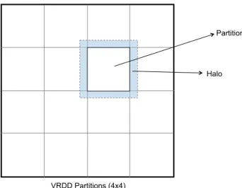
Spark’s RDD is that VRDD allows the user to access the data outside the current
partition. The region overlapped with neighbor partitions is called
halo
(see
Fig-ure 1). In many scientific computing and image processing algorithms, computations
often require accessing its local neighbor data, for example, spatial image filtering.
Partition
Halo
VRDD Partitions (4x4) Fig. 1.VRDD partitions and halo.
Because a VRDD allows accessing neighbor data using halo, computing tasks can be
distributed to different nodes and processed independently. More detailed discussion
about halo is given in section 3.4.
Similar to an RDD, a VRDD can be constructed using the
parallelize
command
with a tag “VISPARK” as follows:
VisRDD = SparkContext.parallelize(inData, Tag="VISPARK", In=4)
When a VRDD is created, the user can specify the number of partitions. Unlike Spark,
which only allows partitioning of the current data, Vispark provides two partitioning
strategies:
input
and
output
splits.
The input split creates the partitions of the
current VRDD data, and the number of partitions can be assigned using an
In
tag.
In the example shown above,
In=4
implies that VisRDD is created with the input
data,
inData
, which will be split into four partitions.
The output split creates the partitions of the
output
VRDD data, which is not
defined in the current VRDD but will be newly generated by the transformations (e.g.,
mappers, reducers, filters). In the following example,
Out=(2,2)
is a 2D partitioning
of the output VRDD that generates four partitions in total. (Note that
multidimen-sional partitioning is available.) If only the output split strategy is used, the entire
input data will be broadcast to each worker process without partitioning.
VisRDD = SparkContext.parallelize(inData, Tag="VISPARK", Out=(2,2))
The input and output split strategies are inspired by the parallel processing model in
Vivaldi language [10] where parallel tasks are generated based on the combination of
input and output data decomposition. By allowing output split, more flexible
par-allel programming is possible in Vispark (for example, screen-decomposition volume
rendering can be implemented by partitioning the output VRDD).
VRDDs can be created from storage sources supported by Spark, such as local file
systems and HDFS. The following example creates a VRDD by reading large binary
data from HDFS (the server’s IP address is 10.20.1.1) located under the directory
Data
:
VisRDD = SparkContext.binaryFiles(‘hdfs://10.20.1.1/Data’, tag="VISPARK")
In order to handle large binary data in Vispark, we provide the Vispark HDFS data
uploader. The uploader splits the input data into a user-specified number of partitions
(or aligned to user-specified partition size) and store them in HDFS with metadata
for neighbor information. For example, if a 2048
×
2048
×
2048 3D volume is given,
and the user splits this volume into 8 slices along each dimension, then each partition
is a 256
×
256
×
256 3D block, and the metadata stores the 8
×
8
×
8 grid information.
Each data partition must be smaller than the predefined maximum size based on the
size of GPU memory.
Vispark uses its own data partitioning schemes as introduced above, but it relies
on Sparks task scheduler for data distribution. Each data partition is assigned to a
Vispark worker process, and if there are more partitions than Vispark workers then
each worker processes multiple partitions sequentially. Vispark controls the maximum
concurrent worker processes assigned to the same GPU (i.e., the number of workers
per computing node) in order to avoid running out of GPU memory.
3.3. Vispark mapper (
vmap
).
Vispark provides GPU-accelerated processing
via mappers because many compute-intensive visual computing tasks can be
imple-mented in the mapper function and the shuffle-reducer stages can be skipped. A
Vispark GPU mapper can be implemented using Vispark’s Python-like language
syn-tax, and its execution can be initiated using a
vmap
transformation function. An
example of mapper execution is shown below:
VisRDD = VisRDD.vmap(mip(data, x, y).range(512, 512))
In this example, the input VisRDD is processed using the mapper function
mip()
,
and the new 2D VisRDD of size 512
×
512 will be generated as a result of this mapper
transformation.
The
range
parameter can be used as in this example to specify
the dimension of the output VRDD. If
range
is not defined, the output VRDD will
have the same size as the input VRDD.
data, x, y,
and
z
are Vispark’s predefined
variables designated to the mapper’s parameters–
data
is the handle for the current
RDD’s data array, and
x, y,
and
z
are the array index to which the mapper function
is applied.
The language syntax of the Vispark GPU mapper is similar to that of the
con-ventional Python except a few domain-specific functions and language definitions.
For example, Code 2 shown below is an example of Vispark GPU mapper
implemen-tation for maximum intensity projection (MIP) volume rendering. In this example,
orthogonal iter
is used to walk along the viewing ray for volume rendering, and
point query 3d()
sampling function is used to access the array data. (A more
de-tailed explanation about Vispark’s domain-specific functions will be given below.)
Code 2
Vispark mapper example of MIP volume rendering. 1 def mip ( volume , x , y ) :
2 s t e p = 1.0 3 l i n e _ i t e r = o r t h o g o n a l _ i t e r ( volume , x , y , s t e p ) 4 5 max = 0.0 6 for e l e m in l i n e _ i t e r : 7 val = p o i n t _ q u e r y _ 3 d ( volume , e l e m ) 8 if max < val : 9 max = val 10 11 z _ v a l = l i n e _ i t e r . g e t _ d e p t h () 12 13 r e t u r n (( x , y ) , ( z_val , max) )
The Vispark mapper code is translated to GPU code
just-in-time
when the
map-per is executed by
vmap
. Code 3 is a CUDA code translated from Code 2 by the
Vispark translator. Because Vispark follows the language syntax similar to Python,
variable types are not declared explicitly in the mapper code. When the mapper
function is executed, necessary variable types are determined dynamically and the
Vispark translator will add the variable types in the translated CUDA code. For
example, the data type of
val
is determined as
float
in Code 3 because the
re-turn type of the data query function (i.e.,
point query 3d()
) returns float value.
VISPARK DATA RANGE
shown in Code 3 is a predefined Vispark data type to define the
shape of data. The input data type for
volume
in Code 3 is determined as
short
by the Vispark worker process when VRDD is transferred.
RESULT DTYPE
is another
Vispark predefined data type for key-value pairs in mapper’s return data. Note how
Vispark’s Python-like syntax is translated into C-like CUDA syntax; for example,
Python-style
for
loop for orthogonal iterator in Code 2 is converted to C-style
for
loop in Code 3.
Code 3
CUDA MIP volume rendering code translated from Code2.
1 _ _ g l o b a l _ _ v o i d m i p s h o r t ( R E S U L T _ D T Y P E * rb , V I S P A R K _ D A T A _ R A N G E * r b _ D A T A _ R A N G E , s h o r t* volume , V I S P A R K _ D A T A _ R A N G E *
v o l u m e _ D A T A _ R A N G E , int x_start , int x_end , int y_start , int y _ e n d ) { 2 3 int x = t h r e a d I d x . x + b l o c k D i m . x * b l o c k I d x . x + x _ s t a r t ; 4 int y = t h r e a d I d x . y + b l o c k D i m . y * b l o c k I d x . y + y _ s t a r t ; 5 6 if( x _ e n d <= x || y _ e n d <= y )r e t u r n; 7 l i n e _ i t e r l i n e _ i t e r ; 8 f l o a t s t e p ; 9 f l o a t max; 10 f l o a t z _ v a l ; 11 s t e p = 1 . 0 ; 12 l i n e _ i t e r = o r t h o g o n a l _ i t e r ( volume , x , y , step , v o l u m e _ D A T A _ R A N G E ) ; 13 14 max = 0; 15 for(f l o a t 3 e l e m = l i n e _ i t e r . b e g i n () ; l i n e _ i t e r . v a l i d () ; e l e m = l i n e _ i t e r . n e x t () ) { 16 f l o a t val ;
17 val = p o i n t _ q u e r y _ 3 d <float>( volume , elem , v o l u m e _ D A T A _ R A N G E ) ;
18 if( max < val ) { 19 max = val ; 20 } 21 } 22 z _ v a l = l i n e _ i t e r . g e t _ d e p t h () ; 23 rb [( x - r b _ D A T A _ R A N G E - > b u f f e r _ s t a r t . x ) +( y - r b _ D A T A _ R A N G E - > b u f f e r _ s t a r t . y ) *( r b _ D A T A _ R A N G E > b u f f e r _ e n d . x -r b _ D A T A _ R A N G E - > b u f f e -r _ s t a -r t . x ) ] = R E S U L T _ D T Y P E ( x , y , z_val , max) ; 24 r e t u r n; 25 }
Once the Vispark mapper function is translated into the CUDA source code, the
VRDD worker process prepares the GPU data and launches the CUDA kernel. The
worker process estimates the total GPU memory size required by the mapper code
and dynamically allocates the GPU memory per data partition. Since the mapper’s
output can be a combination of multiple data items, such as a list of key and values,
the output buffer size should be estimated during the CUDA translation time by
analyzing the mapper code. Once required GPU memory is allocated, the worker
process performs a host-to-device memory copy and launches the CUDA kernel for
the compiled CUDA source code. Once the GPU computation is completed, the
result will be copied back to the CPU memory. We used PyCUDA to coordinate
GPU processing in Python.
Vispark provides domain-specific functions specifically designed for array data
access and numerical computations often used in scientific computing and image
pro-cessing. Such functions can be used only in the GPU mapper code and are translated
into CUDA device functions. Some of them are listed below:
•
Samplers: Since the input data are defined on a rectilinear grid (array),
Vispark provides various memory samplers for hardware-accelerated
inter-polation, for example,
point/linear/cubic query nD()
for nearest, linear
interpolation, and cubic interpolation sampling.
•
Differential operators: First- and second-order differential operators, such
as
linear/cubic gradient nD()
and
laplacian()
, are provided for local
differential computing.
•
Iterators: Vispark provides
stl-like
iterators to access local neighbor data for
each data location (detailed discussion will be given in the following section).
•
Shading Models: Vispark provides widely used illumination models, such as
Phong()
and
Diffuse()
, for volume rendering computation.
3.4. Halo communication.
An important feature of Vispark is automatic halo
synchronization that is transparent to the users. Halo communication is crucial in
scientific computing problems because many numerical algorithms use iterative update
solutions via spatial discretization of differential operators. In Vispark, the user can
simply attach the
halo
command to the mapper function using a dot “.” operator
with the halo size and type when the mapper is called in order to activate halo
synchronization between workers. The Vispark translator can detect whether the
mapper requires halo synchronization or not by checking the presence of the
halo
command. If the halo command is used with a mapper, then halo synchronization is
activated right before the mapper execution. The following is an example of mapper
execution using a halo command:
VisRDD = VisRDD.vmap(filter(data, x, y).halo(simple, 3))
The usage of
halo
command is as follows:
halo( halo type, halo size )
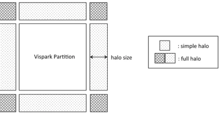
There are two types of halo,
simple
and
full
. Simple halo is the neighbors along
canon-ical directions, such as top, bottom, left, and right directions for 2D and additional
front and back directions for 3D. Full halo is the complete eight directions for 2D and
26 directions for 3D. For example, a finite difference method using central difference
only requires simple halo. However, a convolution filter, such as the Gaussian filter,
requires full halo to access a rectangular neighbor region. The halo size is the width
measured from the edge of the partition to the end of the halo region (see Figure 2).
Vispark’s halo synchronization is implemented using socket communication. There
is a dedicated process that handles halo communication, i.e., the
halo manager
. When
Vispark is started, the halo manager process is launched and waits for halo requests
from workers. Halo synchronization consists of two steps: the first step is workers
sending out halo data to the halo manager (scatter), and the next step is workers
collecting halo data from the halo manager (gather). We separated these steps to
halo size
: simple halo : full halo Vispark Par33on
Fig. 2. 2D halo example.
avoid race conditions, meaning that the first step must be completely finished (i.e.,
halo manager should collect all the halo data from workers before responding to
halo requests). Vispark effectively avoids disk-based shuffle operations by employing
socket communication between workers via the halo manager. We observed that the
proposed socket-based halo communication can effectively reduce the communication
time in our experiments (section 4).
3.5. Neighborhood iterators.
One novel feature of Vispark is that it provides
a programming abstraction for accessing local neighbor data in the mapper. This
does not fit well with the conventional data-parallel MapReduce programming model
because the mapper is designed intentionally to process each individual data element
without knowing its spatial neighborhood. However, this programming model
signif-icantly restricts the application of MapReduce on many array-based scientific data
processing problems. Therefore, we provide
Iterator
, which walks over the neighbor
of each data element in the mapper. Code 4 shows an example of Gaussian filter
im-plementation using a plane iterator (line 6) that covers a (2*kernel+1)
×
(2*kernel+1)
2D range centered at the current data element location (x,y) on the input array (in
this example,
data
). In order to use the plane iterator, the user first defines the halo
type and size depending on the task. In this example, a 2D plane iterator is used to
collect local pixel values to compute a 2D convolution. Therefore, the halo type is
full
, and the size is the same as the Gaussian filter’s kernel size (line 22). Then, each
data element defined in each iterator region can be visited sequentially using a
for
loop without manually computing the index of the data location (line 7).
Code 4
Vispark Gaussian filter implementation using a plane iterator. 1 def g a u s s i a n _ f i l t e r ( data , x , y , dimx , dimy , kernel , s i g m a ) :
2 ret = 0.0 3 val = 0.0 4 PI = 3 . 1 4 1 5 9 2 5 ssq = s i g m a * s i g m a 6 i t e r = p l a n e _ i t e r ( x , y , k e r n e l ) 7 for e l e m in i t e r : 8 val = p o i n t _ q u e r y _ 2 d ( data , e l e m ) 9 dx = e l e m . x - x 10 dy = e l e m . y - y
11 if( e l e m . x >= 0 and e l e m . y >= 0 and e l e m . x < d i m x and e l e m . y < d i m y ) :
12 ret += val * ( 1 . 0 / ( 2 . 0 * PI * ssq ) * e x p f ( -( dx * dx + dy * dy ) / ( 2 . 0 * ssq ) ) )
13 r e t u r n (( x , y ) , ret ) 14 15 if _ _ n a m e _ _ == " _ _ m a i n _ _ " : 16 sc = S p a r k C o n t e x t ( a p p N a m e = " G a u s s _ 2 d " ) 17 img = I m a g e . o p e n ( i n p u t _ n a m e ) 18 d i m y = img . s i z e [1] 19 d i m x = img . s i z e [0] 20 img = n u m p y . f r o m s t r i n g ( img . t o s t r i n g () , d t y p e = n u m p y . u i n t 8 ) . r e s h a p e ( dimy , d i m x ) 21 p i x e l s = sc . p a r a l l e l i z e ( img ,64 , Tag = " V I S P A R K " , In =(16 ,8) )
22 p i x e l s = p i x e l s . v m a p ( g a u s s i a n _ f i l t e r ( data , x , y , dimx , dimy , k e r n e l s i z e , s i g m a ) . r a n g e ( dimx , d i m y ) . h a l o ( full , k e r n e l s i z e ) )
23 r e s u l t = p i x e l s . c o l l e c t ()
It is worth noting that introducing Iterator in Vispark not only adds flexibility
to the MapReduce programming model but also improves the system performance
significantly, especially memory footprints and running time. When the conventional
MapReduce programming model is used, a common approach to implement algorithms
for neighbor access is to generate multiple copies of input data for each neighbor
location. Assume the input data are defined on a 2D array (i.e., 2D image). In order
to access the data on the location (i+1, j) from the current location (i, j), we duplicate
the input image and assign the key (i, j) to the data value at the location (i+1, j)
on one image and at the location (i, j) on the other image, respectively. Then after
shuffling key-value pairs generated by the mapper, the data value at (i, j) and (i+1,
j) will be grouped and assigned to the same key (i, j). Therefore, the reducer can
collect the list of neighbor data values for each key and perform the merging operation.
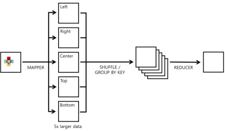
Figure 3 shows that the mapper generates five copies of the input data for the center
and its four neighbor directions (i.e., left, right, top, and bottom) for key-value pairs.
By doing that, the size of the output of the mapper grows linearly with the size of
the local neighbor access required by the algorithm, which is unnecessarily inefficient.
For example, in order to apply Gaussian blur to a 2D image of 512 MB with a kernel
radius of 5, the mapper should generate an intermediate data that is 11
∗
11 = 121
times larger than the input image, which is 61 GB in size in theory!
1This problem
becomes even more severe for higher dimensional data. We can avoid such an absurd
processing scenario by using Vispark Iterator because the mapper can produce the
final output without the reducer. In addition, since the entire shuffle and reduce steps
can be skipped, the total running time can be reduced significantly.
Vispark provides two different types of iterators, i.e., array iterators (line, plane,
and cube) and volume rendering iterators (orthogonal and perspective), listed as
follows:
•
line iter: iterator along an 1D axis-aligned line;
•
plane iter: iterator defined on a 2D axis-aligned rectangle;
•
cube iter: iterator defined on a 3D axis-aligned cube;
•
orthogonal iter: iterator defined on a 3D viewing ray for orthogonal
projec-tion;
•
perspective iter: iterator defined on a 3D viewing ray for perspective
projec-tion.
Note that orthogonal-perspective iterators are designed specifically for volume
ren-dering using ray casting. For each viewing ray, the iterator marches along the ray
from the entrance to the exit point for a given 3D volume (Figure 4, right).
1This shuffling memory overhead can be minimized by usingreduceByKeyinstead ofgroupByKey
if the local filter is a linear weighted sum of its neighbor values.
MAPPER SHUFFLE /
GROUP BY KEY REDUCER
Left Right Center Top Bottom 5x larger data
Fig. 3. Example of conventional MapReduce image processing using a 2D filter kernel (four directions). Perspective Iterator perspective_iter(vol,x,y,step) step view plane Plane Iterator plane_iter(center,radius) radius center
Fig. 4. Iterator examples. Left: plane iterator; right: perspective iterator.
3.6. Vispark translator.
Vispark was developed based on PySpark, a Python
wrapper for Spark. Even though Vispark employs Python-like syntax, it cannot be
executed by PySpark because the GPU mapper and Vispark-specific functions are not
compatible with PySpark. In order to run a Vispark program, the Vispark translator
should translate the input Vispark source code to intermediate code as follows: First,
the Vispark
main
code is translated into the intermediate Python code that PySpark
can execute. Next, the Vispark mapper functions are classified as either native Python
or Vispark code, and Vispark mapper code will be translated into corresponding
CUDA GPU code. Then, the mappers and reducers will be executed either on the
CPU or the GPU depending on the type of its target architecture. The Vispark
runtime system automatically will handle task offloading and memory synchronization
for the GPU.
4. Results.
Vispark is developed based on Spark version 1.2.1. We modified
the source code of PySpark, a Python binding for Spark, with external modules, such
as PyCUDA and NumPy, for GPU processing and array data handling in Python.
We also modified
spark-submit
, which is Spark’s job submission script, to enable
distributed job scheduling on a cluster system. Our prototype system is implemented
and tested on an 8-node cluster system where each node is equipped with an
octa-core Intel Xeon CPU, 32 GB main memory, and an NVIDIA GTX TITAN with
3072 CUDA cores and 12 GB graphics memory. We tested four representative visual
computing benchmark problems, such as Gaussian image filtering, 3D volume
render-ing, K-means clusterrender-ing, and heat transfer simulation, for performance assessment of
Vispark.
4.1. Gaussian filter.
We picked a Gaussian filter as an example of a class of
image processing problems using local neighbors. We compared three different Spark
implementations (pixel-based, patch-based with Spark shuffle, and patch-based with
socket communication) and the proposed Vispark implementation. In the pixel-based
Spark implementation, we designed a map function in such a way that each pixel
re-turns a list of key-value pairs in which the key is the neighbor pixel location within the
filter kernel range and the value is the current pixel value multiplied by the Gaussian
weight based on the distance from the current pixel to the neighbor pixel. You can
think of this as scattering the current pixel value with the corresponding Gaussian
weight to its neighbor pixels so that the convolution computation can be done in the
reducer. The list returned by the mapper is decomposed into individual key-value
pairs by the
flatMap
function. Finally,
reduceByKey
calls the reducer function to
sum up all the values having the same key. The patch-based with Spark shuffle uses
key-patch pairs by decomposing the input image into nonoverlapping patches and each
mapper process gets a patch as an input. In this implementation, the mapper should
walk over the entire patch and compute convolution using Gaussian weights. In order
to handle boundary cases, another mapper should manually cut and exchange halo
regions in Spark’s shuffle/sort stage. You can think of this as a user implementation
of halo exchange using Spark. The path-based with socket communication is an
ex-tension of the patch-based Spark by replacing the disk-based shuffle communication
with the socket-based network communication for halo exchange. In this
implemen-tation, socket communication is implemented in the user-defined mapper function. In
the Vispark implementation, socket communication is implemented in the Spark
sys-tem, and the mapper can directly compute the convolution with the Gaussian kernel
using a built-in iterator on GPUs without a reducer. Therefore, users just need to
implement mapper functions and call them using
vmap
in the main function without
explicitly managing halo communication in the user code.
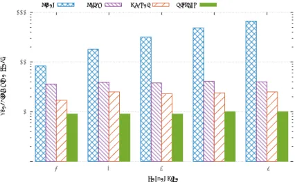
Figure 5 shows the execution time of the Gaussian filter using Spark and Vispark
on the input image with a size of 12125
×
3600 pixels. The performance of Vispark
improves as the kernel size increases, up to around 66 times faster than pixel-based
Spark implementation on a 13
×
13 kernel.
This is due to the fact that Spark’s
system overhead is a dominant factor for a small kernel size, but the problem becomes
compute-bound for a large kernel size. Therefore, GPU-acceleration plays a significant
role in overall performance. Table 1 shows the I/O data size required to communicate
in each implementation. It is shown that the execution time is significantly decreased
for patch-based implementations. This is because the shuffle stage in pixel-based
implementation increases the shuffle data size by kernel*kernel times, but the
patch-based implementation only exchanges halo regions. The socket-patch-based implementations
further reduce the communication time by avoiding shuffle overhead of Spark and disk
I/O. This also shows that Vispark’s architecture improvements play another important
role in system’s performance.
1 10 100 1000
5 7 9 11 13
Execution Time (sec)
KerQel Size
Pixel Patch Socket Vispark
Fig. 5.Running times of Gaussian filtering in different kernel sizes (in seconds, log scale).
Table 1
The data size required for communication (shuffle or socket) in MB. Pixel Patch Socket Vispark Shuffle read
(Socket recv) 2867 54 1.1 1.1 Shuffle write
(Socket send) 2457 62 1.7 1.7
4.2. Volume rendering.
We implemented parallel direct volume rendering as
a representative example for samplers and iterators in Vispark. The proposed parallel
implementation is based on data decomposition and ray casting; that is, the input
volume is decomposed and distributed, rendered in parallel, and the rendered images
are combined to generate the final result. Ray casting walks along each ray per output
pixel, samples the input volume, and applies transfer functions and alpha composition
to generate the final pixel color. For the comparison, we implemented the same volume
rendering method using Spark. Spark leverages data parallelism by partitioning the
input volume—each worker generates a partially rendered image for the given data
partition—but the worker process handles a group of rays (i.e., one ray per pixel in
the output screen) in a serial fashion due to a limited number of parallel cores in
each node. On the other hand, Vispark can implement the proposed parallel volume
rendering using iterators (e.g., perspective and orthogonal) and samplers. In addition,
a Vispark worker leverages pixelwise parallelism using the GPU—a Vispark worker
generates a partially rendered image as in Spark, but each ray is assigned to a GPU
core so that the rendering can be done in parallel.
After the mapper stage, intermediate rendered images need to be combined to
the final resulting image. We implemented the binary-image swap composition using
the iterative shuffle and reducer in Spark and Vispark. In the shuffle stage, each pair
of images is assigned the same key value so that the reducer receives two images to be
merged. This process is repeated
log
2N
times for
N
images so that the entire set of
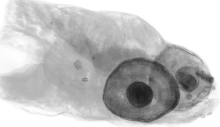
images are combined into the final image. In our experiment, we used the zebrafish
volume data for which the dimension is 1856
×
1612
×
3240 and the output framebuffer
size is 2048
×
2048 pixels. Figure 6 is a rendered image using the Vispark ray-casting
Fig. 6.Ray-casting volume rendering of a zebrafish volume dataset.
Table 2
Running time of ray-casting volume rendering (in seconds). Spark Vispark Number of partitions 64 32 16 8
Rendering time 4320 6120 11160 60 Composition time 265 222 184 155
volume renderer. As shown in Table 2, Vispark is about 72 times faster in rendering
time and about 1.7 times faster in compositing time compared to Spark. Vispark
outperforms Spark in rendering time due to its GPU parallel performance. Vispark
also shows better composition time because fewer intermediate images need to be
merged. Spark can reduce composition time by using large data partitions, but this
significantly will increase the rendering time, which makes the entire running time
much slower.
4.3. K-means clustering.
K-means clustering is a commonly used benchmark
program to test the performance of iterative tasks on MapReduce. We implemented
the algorithm in Spark and Vispark using in-memory cache. The input dataset is
3 million of 784 dimensional points, and we tested using different clustering numbers,
ranging from 20 to 320. The input data are read from HDFS, and we measured the
first and the rest of the iterations separately to show the effect of Spark’s in-memory
cache (i.e., Spark reads the data from disk in the first iteration but the data resides
in memory and is reused in the following iterations).
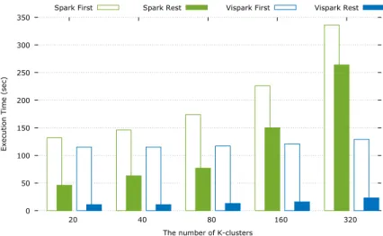
Figure 7 shows the running time of K-means clustering iterations.
The first
iteration shows the running time with the overhead of data loading from the disk.
This can be considered as the running time of K-means clustering on a conventional
Hadoop system, which does not support in-memory cache. As shown in this graph, the
first iteration times of Spark and Vispark differ by only around 10% for K = 20, but
Vispark outperforms Spark by a large margin as the cluster number increases. For 320
clusters, Vispark’s first iteration is more than 2 times faster than that of Spark. The
rest iteration time for K = 320 shows that Vispark largely outperforms Spark, up to
about 11.5 times faster, because the main overhead (i.e., disk I/O) is removed by the
in-memory cache effect. Note that as the number of clusters increases, the difference
0 50 100 150 200 250 300 350 20 40 80 160 320
Execution Time (sec)
The number of K-clusters
Spark First Spark Rest Vispark First Vispark Rest
Fig. 7.Running time comparison of K-means clustering iterations.
between the first and the rest iteration time in Spark (the gap between nonfilled and
filled green bars) is reduced. This is because the K-means algorithm is compute-bound
for a large number of clusters. It means that even though in-memory cache in Spark
can improve the running time of iterative tasks significantly, this benefit is applicable
only to computationally simple problems. If the task is compute-bound, then the
difference between Hadoop and Spark may not be large. In such a case, Vispark
can be a solution because the disk I/O overhead can be suppressed effectively by
in-memory cache in Spark, while the computing overhead can be minimized by the GPU
in Vispark. As a result, Vispark can be up to 14.6 times faster than the conventional
Hadoop for compute-intensive iterative tasks.
4.4. Heat transfer simulation.
Heat transfer simulation is a representative
example of a scientific computing problem that uses an iterative numerical solver with
halo communication. The simulation solves the heat equation (Equation 1) where the
derivatives are approximated using a central difference discretization scheme.
(1)
∂u
∂t
=
h
2∂
2u
∂x
2+
∂
2u
∂y
2+
∂
2u
∂z
2We ran our experiment on a 4000
×
4000
×
2000 rectilinear grid, which is 128 GB
in raw data size for a single precision floating point, and we split the data into 256
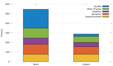
blocks so that each block is 512 MB in size. Figure 8 shows the in-depth analysis of
the running time of a heat transfer simulation. Each running time is broken down into
five groups: communication time, computing time, preparation time, serializer time,
and Spark system overhead. We compared Spark and Vispark implementations of a
heat equation solver where the main differences are communication and computation
types. The Spark heat equation solver uses Spark shuffle for halo communication
and CPU computation. On the other hand, Vispark uses socket-based halo
com-munication and GPU computation. The Vispark heat equation solver (purple bars
in Figure 8) is faster than the Spark solver, but the difference is not large, which
is due to the fact that the heat transfer computation is not compute-bound and all
the GPU overhead (e.g., context and memory management) is included in Vispark’s
computing time. The performance benefit of Vispark implementation mainly comes
0 100 200 300 400 500 600 Spark Vispark Time(s) SparkOverhead Serializer Heatflow Other Process Shuffle
Fig. 8.Running time analysis of heat transfer simulation, showing the relative cost of comput-ing to communication.
from the difference in communication performance (blue bars in Figure 8). The shuffle
communication in Spark is significantly more expensive compared to the socket-based
halo communication in Vispark.
4.5. Discussions.
One of the main contributions of the proposed work is
providing flexible and easy-to-use MapReduce programming tools that hide all the
complicated data and computing resource management from the user, such as halo
communication, GPU kernel execution, and CPU–GPU data transfers. In addition,
Vispark provides various high-level domain-specific functions often used in
visualiza-tion and computing problems, which further saves programmers the effort of writing
long and complicated code. To assess the usability of the proposed programming
lan-guage, we compare source lines of code (SLOC) of a heat transfer simulation written in
Spark and Vispark (see Table 3). In the main function, SLOC of Vispark
implementa-tion is around one-third of the Spark-based implementaimplementa-tions. That is mainly because
Vispark provides a VRDD constructor that automatically analyzes input file types to
leverage distributed file format in HDFS, but Spark does not support such functions;
therefore, the user must handle the file I/O manually. For computation, socket-based
Spark using user-provided CUDA code requires more lines than the other
implemen-tations. This is because the Python implementation and CUDA implementation of
a heat equation solver are almost the same, so Python-based Spark implementations
(i.e., Spark and Spark Socket) and Vispark show the same SLOC, but Spark with
CUDA source code requires GPU device and memory management code to launch
CUDA source code in Python mapper code in Spark. For communication,
socket-based Spark implementations require more than twice the code length as in naive
Spark implementation because halo data management must be done manually. In
Vispark, there is no extra user-written code for halo communication except passing
the halo size to the mapper function call, which is counted as only one line of code.
We also compared Vispark with an existing GPU MapReduce system. Most of
GPU MapReduce systems reported in the literature were not available for download
to the public, and the most similar system we were able to find was GPMR [20].
GPMR is written in C++ and MPI and requires user-written native CUDA code for
GPU execution, so it is much more optimized for performance compared to Java-based
Table 3
SLOC comparison of heat transfer simulation in Spark and Vispark.
Spark Spark Socket Spark Socket CUDA Vispark Main 65 65 65 20 Computation 15 15 55 15 Communication 125 327 327 1 Table 4
Running time comparison of K-means clustering in GPMR and Vispark (in seconds). Number of clusters 20 40 80 160 320
First iteration GPMR 83 85 88 102 120 Vispark 115 115 117 121 129 Rest iteration GPMR 2 4 7 16 30
Vispark 11 11 13 16 23
Hadoop/Spark. Table 4 shows the running time of K-means clustering on GPMR and
Vispark. Because GPMR is not compatible with HDFS, we manually distributed the
input files to nodes and let the system read the data directly from the local disk. As
for the first K-means iteration, GPMR is up to 25% faster than Vispark for the smaller
cluster number (K = 20) because the system overhead dominates the total running
time and GPMR has an unfair advantage in the experiment setup. GPMR does not
use HDFS; therefore, the disk access is much faster, and C++-based implementation
introduces less system overhead for initialization and management of task (e.g.,
man-aging Java virtual machines and processes for task execution). However, if the number
of clusters increases (e.g., K = 320), computation becomes dominant and both
sys-tems show similar performance. As for the rest of the iterations, GPMR shows a much
higher performance than Vispark due to the fact that GPMR’s K-means is based on
highly optimized handwritten CUDA code, for example, leveraging shared memory
and local reduction, while Vispark’s K-means relies on compiler-translated CUDA
code and CPU-based reduction. Furthermore, GPMR leverages CUDA streaming
for processing multiple blocks, but Vispark has some overhead in GPU context and
memory management (due to the limitation of PySpark). Even though Vispark is
a more general system and is not specifically optimized for handwritten GPU code
execution, its performance is comparable to or even better than GPMR for the larger
cluster number (e.g., K = 320) because GPMR does not fully support key-value array
data type, and therefore, it requires more computations as the key size increases. It is
also worth noting that programming in GPMR is more difficult compared to Vispark
because the user must write native CUDA code as well as driver code in C++. In
summary, Vispark demonstrated that its computing performance is comparable to
that offered by the highly optimized C++-based GPU MapReduce system with much
less programming effort.
Even though Vispark introduced significant performance improvement over Spark,
our proposed system has some limitations as well. The current system provides
GPU-acceleration in the mapper function only and shuffling (between mapper and reducer)
is still relying on the conventional disk-based sorting provided by Spark. In the future,
we plan to employ a GPU-based sorting algorithm to accelerate shuffling. Another
limitation is that the current GPU implementation is not optimal, meaning that every
time the CPU worker offloads the task to the GPU, GPU memory has to be newly
allocated. We are planning to implement GPU in-memory processing by reusing GPU
memory so that CPU-GPU data communication can be minimized.
5. Conclusion.
In this paper, we introduced
Vispark
, a GPU-accelerated
distributed visual computing system. Vispark provides a high-level MapReduce
lan-guage, which is similar to Python, provides novel data and processing abstractions,
such as VRDD, iterators, and socket-based automatic halo communication, for
GPU-accelerated local-neighbor access in MapReduce, and allows users to easily implement
visual computing algorithms in a MapReduce framework. In future work, we will
improve the performance of GPU processing in Vispark by implementing GPU
in-memory cache and pipelining. Testing Vispark on a large-scale cluster system is on
our to-do list.
REFERENCES
[1] A. Abbasi, F. Khunjush, and R. Azimi,A preliminary study of incorporating GPUs in the Hadoop framework, in Proceedings of the 16th CSI International Symposium on Computer Architecture and Digital Systems (CADS), IEEE, 2012, pp. 178–185.
[2] Apache,Hadoop,https://hadoop.apache.org/.
[3] R. Appuswamy, C. Gkantsidis, D. Narayanan, O. Hodson, and A. Rowstron,Scale-up vs scale-out for Hadoop: Time to rethink?, in Proceedings of the 4th Annual Symposium on Cloud Computing, SOCC ’13, New York, ACM, 2013, pp. 20:1–20:13, http://doi.acm.org/ 10.1145/2523616.2523629.
[4] M. Armbrust, R. S. Xin, C. Lian, Y. Huai, D. Liu, J. K. Bradley, X. Meng, T. Kaftan, M. J. Franklin, A. Ghodsi, et al.,Spark SQL: Relational data processing in Spark, in Proceedings of the 2015 ACM SIGMOD International Conference on Management of Data, ACM, 2015, pp. 1383–1394.
[5] C. Basaran and K.-D. Kang,Grex: An efficient MapReduce framework for graphics process-ing units, J. Parallel Distributed Comput., 73 (2013), pp. 522–533.
[6] G. Brumfiel, High-energy physics: Down the petabyte highway, Nature, 469 (2011), pp. 282–283, http://dx.doi.org/10.1038/469282a.
[7] J. Buck, N. Watkins, G. Levin, A. Crume, K. Ioannidou, S. Brandt, C. Maltzahn, N. Polyzotis, and A. Torres,Sidr: Structure-aware intelligent data routing in Hadoop, in Proceedings of the International Conference on High Performance Computing, Network-ing, Storage and Analysis, ACM, 2013, p. 73.
[8] J. B. Buck, N. Watkins, J. LeFevre, K. Ioannidou, C. Maltzahn, N. Polyzotis, and S. Brandt,SciHadoop: Array-based query processing in Hadoop, in Proceedings of 2011 International Conference for High Performance Computing, Networking, Storage and Anal-ysis, ACM, 2011, p. 66.
[9] B. Catanzaro, N. Sundaram, and K. Keutzer,A MapReduce framework for programming graphics processors, in Workshop on Software Tools for MultiCore Systems, 2008. [10] H. Choi, W. Choi, T. Quan, D. G. Hildebrand, H. Pfister, and W.-K. Jeong,Vivaldi: A
domain-specific language for volume processing and visualization on distributed heteroge-neous systems, IEEE Trans. Vis. Comput. Graph., 20 (2014), pp. 2407–2416.
[11] J. Dean and S. Ghemawat,MapReduce: Simplified data processing on large clusters, in Pro-ceedings of the 6th Conference on Symposium on Opearting Systems Design & Implemen-tation, Vol. 6, Berkeley, CA, USENIX Association, 2004, http://dl.acm.org/citation.cfm? id=1251254.1251264.
[12] M. Elteir, H. Lin, W.-c. Feng, and T. Scogland,StreamMR: An optimized MapReduce framework for AMD GPUs, in 17th International Conference on Parallel and Distributed Systems (ICPADS), IEEE, 2011, pp. 364–371.
[13] W. Fang, B. He, Q. Luo, and N. K. Govindaraju, Mars: Accelerating MapReduce with graphics processors, IEEE Trans. Parallel Distributed Systems, 22 (2011), pp. 608–620. [14] Y. Geng, X. Huang, M. Zhu, H. Ruan, and G. Yang,SciHive: Array-based query processing
with hiveQL, in Proceedings of 12th IEEE International Conference on Trust, Security and Privacy in Computing and Communications (TrustCom), IEEE, 2013, pp. 887–894. [15] M. Grossman, M. Breternitz, and V. Sarkar,HadoopCL: MapReduce on distributed
het-erogeneous platforms through seamless integration of Hadoop and OpenCL, in Proceedings of the 27th International Parallel and Distributed Processing Symposium Workshops & PhD Forum (IPDPSW), IEEE, 2013, pp. 1918–1927.
[16] V. Kaynig, A. Vazquez-Reina, S. Knowles-Barley, M. Roberts, T. R. Jones, N. Kasthuri, E. Miller, J. Lichtman, and H. Pfister,Large-scale automatic
recon-struction of neuronal processes from electron microscopy images, Medical Image Anal., 22 (2015), pp. 77–88, http://dx.doi.org/10.1016/j.media.2015.02.001.
[17] D. Laney, 3D Data Management: Controlling Data Volume, Velocity, and Variety, Tech. report, META Group, 2001, http://blogs.gartner.com/doug-laney/files/2012/01/ ad949-3D-Data-Management-Controlling-Data-Volume-Velocity-and-Variety.pdf. [18] M. Lu, Y. Liang, H. P. Huynh, O. Z. Liang, B. He, and R. S. M. Goh,MrPhi: An optimized
MapReduce framework on Intel Xeon Phi coprocessors, IEEE Trans. Parallel Distributed Systems, 26 (2015), pp. 3066–3078.
[19] J. A. Stuart, C.-K. Chen, K.-L. Ma, and J. D. Owens,Multi-GPU Volume Rendering using MapReduce, Presented at 1st International Workshop on MapReduce and its Applications, 2010.
[20] J. A. Stuart and J. D. Owens,Multi-GPU MapReduce on GPU Clusters, in Proceedings of the 2011 IEEE International Parallel & Distributed Processing Symposium, IPDPS ’11, Washington, DC, 2011, pp. 1068–1079, http://dx.doi.org/10.1109/IPDPS.2011.102. [21] D. Tam,Facebook Data Rate,
http://www.cnet.com/news/facebook-processes-more-than-500-tb-of-data-daily/.
[22] H. T. Vo, J. Bronson, B. Summa, J. L. D. Comba, J. Freire, B. Howe, V. Pascucci, and C. T. Silva,Parallel visualization on large clusters using mapreduce, in Proceedings of the IEEE Symposium on Large Data Analysis and Visualization (LDAV), IEEE, 2011, pp. 81–88.
[23] Y. Wang, G. Agrawal, T. Bicer, and W. Jiang,Smart: A MapReduce-like framework for in-situ scientific analytics, in Proceedings of the International Conference for High Perfor-mance Computing, Networking, Storage and Analysis, New York, 2015, ACM, pp. 51:1– 51:12, http://doi.acm.org/10.1145/2807591.2807650.
[24] Y. Wang, W. Jiang, and G. Agrawal,SciMATE: A novel MapReduce-like framework for multiple scientific data formats, in Proceedings of the 2012 12th IEEE/ACM International Symposium on Cluster, Cloud and Grid Computing (Ccgrid 2012), CCGRID ’12, Wash-ington, DC, 2012, pp. 443–450, http://dx.doi.org/10.1109/CCGrid.2012.32.
[25] R. S. Xin, J. Rosen, M. Zaharia, M. J. Franklin, S. Shenker, and I. Stoica, Shark: SQL and rich analytics at scale, in Proceedings of the 2013 ACM SIGMOD International Conference on Management of Data, ACM, 2013, pp. 13–24.
[26] M. Zaharia, M. Chowdhury, T. Das, A. Dave, J. Ma, M. McCauley, M. J. Franklin, S. Shenker, and I. Stoica,Resilient distributed datasets: A fault-tolerant abstraction for in-memory cluster computing, in Proceedings of the 9th USENIX Conference on Networked Systems Design and Implementation, NSDI’12, Berkeley, CA, 2012, USENIX Association, pp. 2–2, http://dl.acm.org/citation.cfm?id=2228298.2228301.
[27] M. Zaharia, M. Chowdhury, M. J. Franklin, S. Shenker, and I. Stoica,Spark: Cluster computing with working sets, in Proceedings of the 2nd USENIX Conference on Hot Topics in Cloud Computing, HotCloud’10, Berkeley, CA, 2010, USENIX Association, pp. 10–10, http://dl.acm.org/citation.cfm?id=1863103.1863113.