A study into automatic speaker verification with aspects of deep learning

with Aspects of Deep Learning

by

Keith A. Jellyman

08/05/2018

A thesis submitted to the UNIVERSITY OF BIRMINGHAM

in candidature for the degree of MSc by Research

Supervisor: Prof. M. Russell

Department of Electronic, Electrical and Systems Engineering School of Engineering

University of Birmingham Research Archive

e-theses repository

This unpublished thesis/dissertation is copyright of the author and/or third

parties. The intellectual property rights of the author or third parties in respect

of this work are as defined by The Copyright Designs and Patents Act 1988 or

as modified by any successor legislation.

Any use made of information contained in this thesis/dissertation must be in

accordance with that legislation and must be properly acknowledged. Further

distribution or reproduction in any format is prohibited without the permission

of the copyright holder.

Advancements in automatic speaker verification (ASV) can be considered to be primarily lim-ited to improvements in modelling and classification techniques, capable of capturing ever larger amounts of speech data.

This thesis begins by presenting a fairly extensive review of developments in ASV, up to the current state-of-the-art with i-vectors and PLDA. A series of practical tuning experiments then follows. It is found somewhat surprisingly, that even the training of the total variability matrix required for i-vector extraction, is potentially susceptible to unwanted variabilities.

The thesis then explores the use of deep learning in ASV. A literature review is first made, with two training methodologies appearing evident: indirectly using a deep neural network trained for automatic speech recognition, and directly with speaker related output classes. The review finds that interest in direct training appears to be increasing, underpinned with the intent to discover new robust ‘speaker embedding’ representations.

Last a preliminary experiment is presented, investigating the use of a deep convolutional neural network for speaker identification. The small set of results show that the network successfully identifies two test speakers, out of 84 possible speakers enrolled. It is hoped that subsequent research might lead to new robust speaker representations or features.

ASR Automatic speech recognition

ASV Automatic speaker verification

DCT Discrete cosine transform

DFT Discrete Fourier transform

DNN Deep neural network

EM Expectation maximisation

EER Equal error rate

GMM Gaussian mixture model

G-PLDA Gaussian-probabilistic linear discriminant analysis HT-PLDA Heavy tailed-probabilistic linear discriminant analysis

JFA Joint factor analysis

LDA Linear discriminant analysis

MAP Maximum a-posteriori

MFCC Mel-frequency cepstral coefficients

minDCF Minimum discrete cost function

T-Norm Test-Normalisation

VAD Voice activity detector

WCCN Within class covariance normalisation

UBM Universal background model

1 Introduction 1

1.1 Thesis Structure . . . 3

2 Automatic Speaker Verification 6 3 Gaussian Mixture Models (GMMs) 8 3.1 Front End Processing (Feature Extraction) . . . 11

3.2 Dynamic Feature Extraction . . . 13

3.3 The Universal Background Model . . . 14

3.4 UBM-MAP Speaker Model Training . . . 15

3.5 Score Normalisation . . . 19

4 I-Vectors 21 4.1 Training the T-Matrix . . . 24

4.1.1 Stage 1 - Prepare Required Statistics . . . 27

4.1.2 Stage 2 - Calculate Posterior Expectation ofw(s) (EM Algorithm) . . . . 28

4.1.3 Stage 3 - UpdateT via Maximisation (EM Algorithm) . . . 32

4.2 T-Matrix Training Overview and I-Vector Extraction . . . 40

4.3 Speaker Verification Scoring and PLDA . . . 43

4.3.1 Probabilistic Linear Discriminant Analysis (PLDA) . . . 44

4.3.2 The Statistical Independence Assumption . . . 47

4.3.3 Gaussian Assumptions: Heavy-Tailed PLDA . . . 49

4.3.4 Gaussian Assumptions: I-Vector Length Normalisation . . . 50

4.3.5 PLDA Conclusions . . . 54

5 Performance Tuning Experiments 57 5.1 Experimental Corpora and Toolboxes . . . 58

5.2 Accuracy Scoring . . . 59

5.3 ASV Hyperparameter Settings and the Voice Activity Detector . . . 62

5.4 GMM-UBM Experiments . . . 64

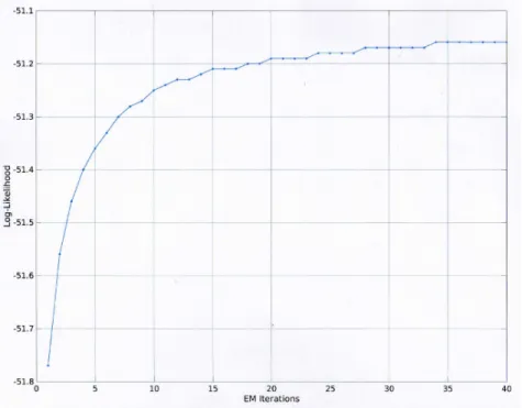
5.4.1 EM UBM Training Iterations . . . 65

5.4.2 Application of the VAD and CMV in the Front-End Process . . . 65

5.4.3 Acceleration Features, Background Training Data, and Model Size . . . . 69

5.5 I-Vector Experiments: T-Matrix Training . . . 73

5.5.1 Results and Analysis . . . 75

5.6 Experimental Conclusions . . . 79

6 Deep Learning 84 6.1 The Indirect DNN-ASR Approach for ASV . . . 86

6.1.1 Performance of the DNN/i-vector Framework and Bottleneck Features . . 91

6.1.2 The CNN/i-vector Framework for Noisy Conditions . . . 94

6.2 Direct Training of DNNs for ASV . . . 100

6.2.1 D-Vectors via DNNs for Speaker ID . . . 100

6.2.2 Speaker Embeddings for End-to-End ASV . . . 105

6.2.3 Performance of D-Vectors and Speaker Embeddings . . . 110

6.3 Preliminary Experiment - Speaker Identification using CNNs . . . 118

6.3.1 Deep Network Architecture and Component Settings . . . 119

6.3.2 Experimental Protocol . . . 122

6.3.3 Results and Analysis . . . 124

6.4 Deep Learning Conclusions . . . 126

7 Conclusions and Recommendations 130

1.1 Exponentially decreasing percentage equal error rates (%EER) across the NIST-SRE trials from 2004 to 2012, with the 2004-05 %EER results taken from [5], and the remaining five years taken respectively from [6, 8–10]. . . 2 2.1 Likelihood ratio-based automatic speaker verification (ASV). . . 6 3.1 Likelihood-ratio based speaker verification system using a single reference

univer-sal background model (UBM). The first stage to training a GMM-UBM ASV, is to (a) train a UBM on a extremely last cohort of background speakers, enabling then, (b) hypothsised speaker models to be then trained using MAP adapted EM training, relative to the central reference UBM. With both the non-hypothesised UBM and hypothesised speaker models trained, likelihood-ratio based speaker verification (c) can then be applied to unknown speech recordings, with yes/no decisions made using a pre-defined score decision threshold. . . 9 3.2 Cepstral feature extraction process. . . 11 3.3 Illustration of how the speaker model Gaussian components are referenced relative

to the universal background model (UBM) via maximum a-posteriori adaptation (MAP). Gaussian componentsC1 andC2 are opportunely adapted by the speaker enrolment features available, withC3 left defined by the original UBM. . . 16 5.1 Example detection error trade-off (DET) curve. . . 60 5.2 Main automatic speaker verification processing stages. . . 62 5.3 UBM log-likelihood probability p(X_|λ) with respect to EM training iterations,

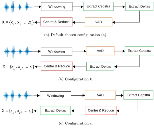
on the male SRE04 training data ‘X’, with 19C+E+19∆+∆E = 40 cepstra, and 512 Gaussian components. . . 66 5.4 The three different front-end configurations considered, with respect to the

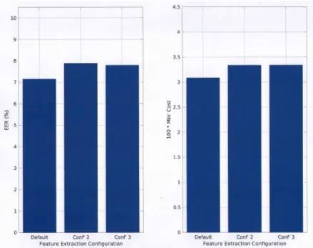
loca-tions of the VAD and cepstral mean variance (CMV) normalisation. . . 67 5.5 Respective %EER and cost performance scores with respect to the specific

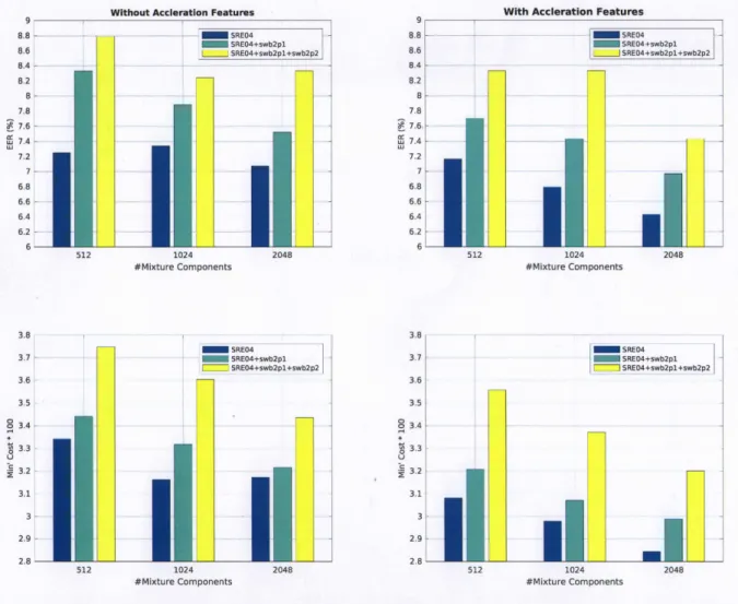
ap-plication of the VAD and CMV within the front-end feature extraction process. The three configurations are defined in Figure 5.5. . . 68 5.6 Percentage EER and cost scores with respect to with, and without acceleration

cepstral features, and the amount of UBM training data (horizontal axis). No energy coefficients are used. . . 70

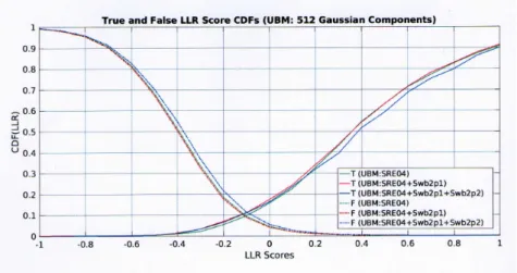
5.7 True and false trial-cumulative distribution LLR score plots, at 512, 1024 and 2048 Gaussian components. Each plot contains the true and false score profile pairs for the UBMs trained incrementally with SRE04 (training), and Switchboard II-Phases 1 and 2 data. . . 72

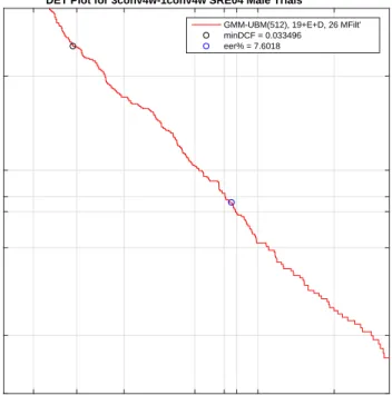
5.8 DET plots showing the ASV i-vector performance with cosine scoring at (a)

1024 and (b) 2048 Gaussian components, on the male NIST-SRE 2005 (3conv4w-1conv4w) reference set, with respect to incrementally increasing the amount of male training data used to estimate the T-matrix. . . 77

5.9 Combined 1024 and 2048 Gaussian component DET plot for ease of comparison,

and for comparing with and without the use of Fisher English male training data in the training of the T-matrix, again on the male NIST-SRE 2005 (3conv4w-1conv4w) reference set with cosine scoring. . . 78 6.1 Illustration of the indirect DNN-ASR architecture taken from [71], where the

output classes of the DNN are defined as the phonetic senone states, which are also effectively the tied-triphone states of an ASR-HMM. The acoustic features are stacked around the current input frame (in practice +/-5 frames [66, 71] context) for input into the DNN. Bottleneck features can also be extracted by restricting the number of nodes in one of the hidden layers, and taking its output as features [56, 72]. . . 88 6.2 The proposed ‘DNN/i-vector’ framework proposed by Lei et al [22], where the

ASR trained DNN is used to more accurately estimate the zero’th order utterance level statistics, and the frame level senone posterior probabilities for alignment. The diagram also illustrates how the features for the ASR-DNN (log-mel filter-banks =xt), are not incumbent on the features used for ASV (e.g., MFCCs + ∆ + ∆∆ =x0_t). . . 90 6.3 Illustration of the CNN-ASR deep network used by McLarenet al[25], for their

alternate CNN/i-vector framework for ASV in noisy conditions. Compared with their original DNN/i-vector framework in [22], the first layer is substituted for a convolutional layer instead. The remainder of the network is unchanged, consist-ing of between 5 to 7 fully connected layers. Followconsist-ing the diagram in [25], only one convolutional filter is shown, but in total they use 200 filters, generating 200 corresponding ‘filter maps’. The filters are convolved with the filterbank spectral image along the frequency access only. The size of the filter used is also larger in practice than shown, with a context of 15 time frames (equal to the CNN in-put), and a height normally of 8 filterbank coefficients. They use non-overlapping max pooling, with a pooling size of 3. In the illustrative figure, this produces a 2-dimensional output vector. . . 96 6.4 Illustration of the background speaker identification DNN used to extract a

d-vectors for a speaker, by averaging the output activations from the last hidden layer. . . 101

6.5 Illustration of the ‘end-to-end’ deep network proposed by Heigold et al [91] for ASV, building on the original d-vector work by Variani et al [23], with an addi-tional logistic regression layer added to learn the cosine speaker model and test utterance d-vector distance scores, and the use of a time-sequence LSTM RNN in place of a DNN. Heigold et al [91] refer to d-vectors as speaker representations, which inspires the very recent work on ‘speaker embeddings’ by Snyderet al[26]. 103 6.6 Illustration of the end-to-end ASV process using speaker embeddings by Snyder

et al[26], with (a) the DNN architecture proposed that maps stacked MFCC to a ‘speaker embedding’ vector, and (b) the ASV scoring process. The objective func-tion L(xtest, xmodel) operates on pairs of embeddings, maximising same speaker embeddings, and conversely minimising pairs of embeddings from different speakers.106

6.7 Summary %EER scores with and without T-norm taken from Varianiet al [23]

(V), Heigold et al [91] (H), and Snyder et al [26] (S), comparing direct DNN training approaches for ASV: V=comparison between d-vector and classic i-vector with T-norm; S=comparisons between classic i-vectors with PLDA scoring, their speaker embedding ASV (DNN), and fusion, whilst varying the enrol and test durations, [1-20s] implies variable between 1 to 20s, and full implies a complete recording; H=d-vector type formulations using either a softmax or a complete end-to-end objective training criterion, substituting the DNN for a LSTM network, and varying the amount of DNN training data from 2M utterances (train 2M) to 22M (train 22M). . . 114 6.8 DET ASV performance graphs highlighting potential score calibration issues with

the current direct training of DNNs for ASV: (a) taken from Variani et al [23], with d-vectors using only 4 “Okay Google” utterances for enrolment; and (b) taken from Snyderet al[26] for pooled 10s, 20s and full recording test conditions, with 1-20s enrolment, and their 102K speaker set for training the i-vector UBM and DNN for speaker embedding extraction. . . 114 6.9 Proposed closed speaker identification task. . . 119 6.10 Illustration of the CNN-DNN network architecture used for speaker

identifica-tion. The first CNN layer is expanded for illustrative purposes, comprising of a convolution+non-linear activation and a max pooling process. The single 3 x 3 example convolutional filter shown for display only, is smaller than the filter used during the experiments, which was 5 x 5 for both CNN layers. In total, 32 filters were used in the first CNN layer, and 64 in the second, generating the equivalent number of respective feature maps. A max pooling group size of 2 x 2 was used for both CNN layers. . . 120 6.11 Activation scores averaged across the two respective test recordings (jebn:A,

jaxv:A), for the network with 44 models (a), and 88 models (b). The two pairs of plots highlight how the network correctly identifies speakers M7029 (model 1), and M7040 (model 2) correctly. . . 125

4.1 I-vector compensated results from Garcia-Romero and Espy-Wilson [10] compar-ing Gaussian (G) and heavy-tailed (HT) PLDA, with length normalisation on the NIST-10 telephony core 5 condition. . . 54

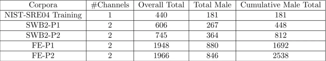
5.1 List of corpora used for training the UBMs and T-matrices in hours

(SWB2-P1=Switchboard 2-Phase 1, FE-P1=Fisher English-Part 1). . . 59 5.2 The reference test set used, which is selected out of the NIST-SRE 2005

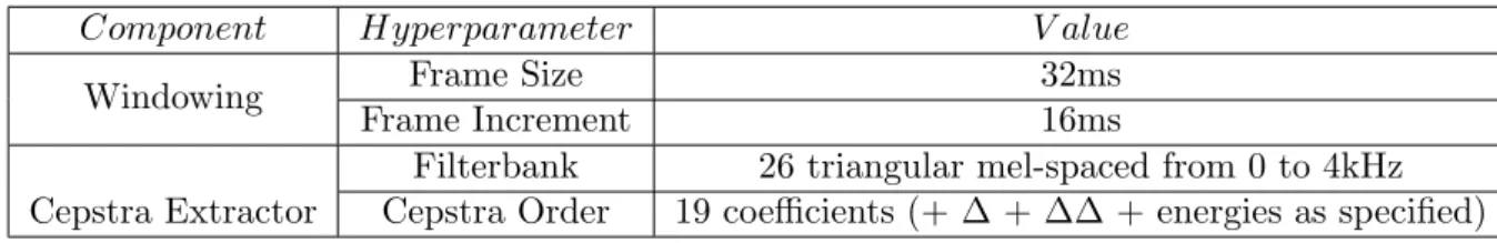
evalu-ation standard trial conditions, where ‘3conv4w‘ is the model training list, and ‘1conv4w’ the test list. . . 59 5.3 Cost scoring equation parameters as defined by NIST-SRE in 2005 [58]. . . 61 5.4 Feature extraction hyperparameter settings. . . 63 5.5 Voice activity detector feature extraction and model hyperparameter settings. . . 64 5.6 The UBM (Gaussian components), T-matrix (rank order), and the feature order

hyperparameter values. The number of Gaussian components in the UBM is investigated at both 1024 and 2048 components. The number of EM training iterations for both the UBM and T-matrix is set at 20. . . 74 5.7 The background male data used to train the UBM, and to estimate the T-matrix.

The UBM data is fixed throughout the experiment, with three corpora used. The T-matrix is incrementally increased, starting with NIST-SRE 2004 (training), then adding Switchboard II-Phases 1 and 2, with last the two Fisher English-Parts 1 and 2. . . 74

6.1 Comparative NIST-SRE primary cost scores taken from [56] on the NIST-SRE

2012 extended clean telephone (core 2) and microphone (core 1) conditions, com-paring indirect DNN-ASR ASV performances using different combinations of the DNN-senone derived UBM and bottleneck features, relative to the classical UBM Mel-cepstral feature (MFCC) i-vector baseline. pcaDCT are alternate acoustic features to MFCC investigated in [56]. . . 93 6.2 Percentage miss at 1.5% false alarm (FA) and percentage equal error rate (%EER)

scores taken from McLaren et al[25] in descending order, derived on the RATS SID 10s-10s (enroll[6x10s]-test) [83] noisy radio re-transmissions, comparing the use of the classic UBM/i-vector extraction [3] to their proposed CNN/i-vector framework, and with fusion. They also make comparisons between using percep-tual linear prediction (PLP), and power normalised cepstral coefficient (PNCC) features. The matched language test set used consists of 85K target and 5.8M impostor trials, from 305 unique speakers. . . 97

6.3 Percentage EER and minimum cost scores for two operating points for gender

dependent models taken from Snyder et al [85], on the NIST-SRE 2010 core

five extended telephony condition, comparing the classic UBM(5297)/i-vector [3] with 5297 Gaussian components, and their TDNN(5297)/i-vector framework. The

minDCF10−3 _{refers to the new NIST-SRE 2010 minimum cost cost operating}

point, with an a-priori hypothesised speaker probability of 0.001. . . 99 6.4 DNN-CNN and front-end log-mel filterbank calculation settings. Rectified linear

units (ReLU) were used as the non-linear activation function for all three layers. 121 6.5 Initial test models and training/test speech data taken from the NIST-SRE 2005

‘3conv4w’ training set [58] . The M7845 test recording was not used due to the recording only containing half the amount of speech to the other two recordings. The M8611 test recording was found to contain no speech at all. . . 122

Introduction

Developing algorithms to automatically recognise individuals from their speech is a challenging task. Speech recordings often contain large amounts of variability, which if not accounted for can severely degrade performance. The sources of these variabilities can include speaker specific types, for example a person’s emotional state, their health, and increase in age over time; transmission channel variabilities, such as coder-decoders (CODECs), and background noise; as well as other recording variabilities, such as phonetic content and duration.

A considerable amount of effort in addressing variability issues though has been made within the specific field of automatic speaker verification (ASV) [1–3]. ASV is about determining whether or not a speech recording was spoken by an enrolled speaker, compared with identification, which is about determining who specifically produced a speech signal out of a set of enrolled speakers.

Figure 1.1 illustrates how the percentage equal error rates (EER) on English telephony speech, over the period of 2004 to 2012, have decreased exponentially. The percentage EER corresponds to when the decision threshold value set, results in an equal percentage of false alarms and miss errors, and is often used as benchmark comparison score. The results presented are taken from the NIST speaker recognition evaluations (NIST-SRE) [4], which have become an almost official standard for comparing leading performances within the ASV research community.

In 2004, Figure 1.1 shows how the equal error rate (EER) performance on NIST-SRE English telephony trials corresponded to around 7.73% [5], dropping exponentially to just under 1% in 2012 [6]. The focus of the latest 2016 evaluation [7] appears to have now moved on to addressing non-English speech.

04 05 06 08 10 12 NIST-SRE Evaluation Years

0 1 2 3 4 5 6 7 8 9 Eq ua l E rr or R at e (% ) 7.73% 4.85% 3.29% 2.10% 1.27% 0.90%

Figure 1.1: Exponentially decreasing percentage equal error rates (%EER) across the NIST-SRE trials from 2004 to 2012, with the 2004-05 %EER results taken from [5], and the remaining five years taken respectively from [6, 8–10].

Figure 1.1 shows how the performance on English telephony can be considered in many respects to be at, or if not very close, to the upper achievable limit. However it can be argued that much of the research focus from 2000 to achieve this performance, has been primarily about developing speaker models, that are capable of capturing variabilities across vast labelled corpora. There has been significantly less importance placed instead, with improving the understanding of speaker specific structures, and in particular the pre-stage feature extraction process. The majority of recognition systems still use cepstral features, which was originally proposed by Furui [11] in 1981.

This observation has as well been made recently in two eminent works. Garcia-Romero [12] for example makes this observation at the beginning of his thesis from 2012, writing that, “Recent advances in speaker recognition are not necessarily due to new or better understanding of speaker characteristics that are informative or interpretable by humans; rather, they are the result of improvements in machine learning techniques that leverage large amounts of data.”

His statement has been followed by Todisco et al [13] at Speaker Odyssey 2016, where they wrote that, “There is more to be gained from the study of features rather than classifiers.” They found that by adopting this approach with their detection of spoofing attacks work, they were able to achieve a 72% relative improvement with their newly proposed perceptually weighted cepstral coefficients. Their paper subsequently won one of the best paper awards.

To help give some impression of the exponential increase in speech training data used, the 2004 NIST evaluation contained approximately 500k gross trials. However the 2012 evaluation has since exceeded 114 million trials, equating to a 228 times increase in size. The extensive NIST speech corpora are usually then expanded even further, by taking advantage of the large amounts of available Switchboard corpora recordings [14].

Therefore despite the exceptional performance achieved with specifically English telephony, auto-matic speaker verification algorithms still remain somewhat susceptible to sources of variability that have not been included in the model training corpora [15], and especially when used in challenging degraded environments.

Referring again to Garcia-Romero’s thesis [12], he shows how in less than benign conditions, performance degrades rapidly. Adding babble noise at 6dB signal-to-noise ratio (SNR), he found that the percentage equal error rate increased ten-fold relative to his original telephony conditions, at 1.43% to 10.7%. If automatic speaker verification algorithms therefore are to become truly robust to unwanted variabilities, then more robust features beyond cepstra are very likely needed. This theme forms the underlying motivation of the work presented.

1.1

Thesis Structure

This thesis begins by first formerly presenting the automatic speaker verification (ASV) task. Following this, a relatively in-depth review of the developments up to, and including the current

state-of-the-art is presented. ASV has seen an extensive amount of research published, the majority of which can be argued has been around developing speaker models and classification techniques, and not in the development of features. However, it is important to review the research published, in order to better understand the limits of the current techniques. The review starts with the pioneering work by Reynolds [16], on Gaussian mixture models (GMMs) with Bayesian adaptation during the mid-’90s, charting the advancements that have eventually led to the development of i-vectors (identity) by Dehak et al [3], in around 2010.

Following the review a series of practical tuning experiments are presented. It is found that published works can sometimes lack in specific implementation details. For example, a lot of publications will usually only write that they have taken whole evaluation data sets, such as NIST-SRE 2004 to 2006 [3], with little or no information on how they pre-screened or prepared the data, and their specific feature calculation details. The experiments presented, attempt to address some of these issues by repeating some of the leading published works [3, 12, 17], as well as hopefully providing a much deeper practical understanding of the limits of the various approaches.

Throughout the experiments presented a fixed reference test set is used. This is done to enable performances differences to be compared between earlier and later recognition approaches. These comparable set of experimental findings are hopefully of value, and contribution in particular, to ASV research community.

With the underlying motivation to discover new robust features beyond cepstra and speaker specific structures, this then motivates the initial investigation into the use of deep learning. Pioneered by LeClun et al [18], deep learning has led to major advancements in image object recognition [19], automatic speech recognition (ASR) [20], and machine translation [21].

Deep learning prescribes a data-driven automated methodology to discovering new features or representations from the raw data [18]. Multiple levels of representation are learnt automatically,

often using large multi-layer neural networks. The higher levels conceptually correspond to higher levels of abstraction, that are hopefully representative of the decision class, and are defined by composition of the lower level representations.

The success of deep learning within automatic speaker recognition research can be viewed as being rather limited to date, when compared to the other communities mentioned. Specifically, research investigating the direct training of deep neural networks (DNNs), where the output classes to be discriminated between are speaker related, has appeared somewhat limited until of very recent. This is most likely attributed to the often limited amounts of enrolment data available per speaker [22]. However, the direct training effectively tasks DNNs to discover new discriminative speaker features or representations.

One of the first published work that has investigated direct training, is by Variani et al [23] in 2014. However their work is limited to using recordings of speakers uttering the fixed phrase “Okay Google”. Much of the related publications appear otherwise to either involve using a ptrained deep neural network for automatic speech recognition [24, 25]. It is only very re-cently, that interest appears to be noticeably increasing, with in particular the work on “speaker embeddings” by Snyder et al [26].

With this in mind, a review of work investigating deep learning in the context of ASV is pre-sented. This is followed by some experimental work, investigating the direct training of a deep convolutional neural network for speaker identification. The work presented is very much a first attempt and much further work is needed, but it is hoped that this might lead in the not too distant future to new robust speaker features, and insight. The thesis then closes with some final conclusions and recommendations.

Automatic Speaker Verification

This chapter outlines briefly speaker verification from an automated research perspective.

Speaker verification is defined as the task of determining whether or not an unknown speech segment was spoken by some hypothesised speaker, and can be considered also as a speaker detection problem. Figure 2.1 shows the typical likelihood ratio implementation adopted for automated systems [1].

Figure 2.1: Likelihood ratio-based automatic speaker verification (ASV).

A raw speech segmentY is first passed through a front-end process to extract hopefully robust speaker dependent features. These features are then processed as an hypothesis test between:

H0 : Y is from hypothesised speaker S,

H1 : Y is not from hypothesised speakerS.

In order then to verify whether or not speech segment Y was uttered by speaker S, the ratio of

the two output hypothesis scores can be then taken: ∧= p(Y|H0) p(Y_|H1)      >=θ acceptH0 < θ rejectH0 (2.1)

where p(Y_|H0) is the probability density function for the true hypothesis H0, evaluated for

observed speech segmentY. Conversely,H1 represents the false hypothesis, that speech segment

Y was not produced by the hypothesised speaker S.

If the likelihood ratio score exceeds or is equal toθ, then the true hypothesis is chosen, otherwise the false hypothesis is selected.

Often the log of the likelihood ratio is then taken [1], giving the final summation score form:

∧= logp(X_|λhyp)−logp(X|λhyp) (2.2)

where p(Y|H0) in practice is represented by p(X|λhyp), with X a sequence of feature vectors

X ={x1, ..., xT}indexed at timet∈[1,2...T];H0is represented by modelλhyp, and the alternate

hypothesis H1 by model λ_hyp.

The notional aim of automatic speaker verification research is to then develop both, robust models to represent the two hypotheses, and feature extractors, such that decision error rate is minimised.

Gaussian Mixture Models (GMMs)

Automatic speaker verification (ASV) has advanced significantly since the mid-’90s, with major advancements appearing to emerge roughly every four years. The technology applied to tele-phony speech is now at a point where banks, and other large global corporations are beginning to use it on a daily basis [27, 28]. It was argued at the start of this thesis, that the focus of ASV research to achieve this level of performance, has been primarily around developing models that are capable of capturing variabilities across vast labelled corpora. Probably the key early instigating work in data-driven speaker models is by Reynolds et al [16], with their work on adapted Gaussian mixture models (GMM) from the mid-’90s.

Reynolds et al [16] proposed the training of a single large GMM based universal background model (UBM), to both capture unwanted variabilities, and to help counter for the often limited amount of hypothesised speaker training data by maximum a-posteriori (MAP) adaptation. The use of a single large UBM also importantly provides a probabilistic reference, allowing speaker models to be compared. Such was the success of this formulation, it essentially still underpins the current state-of-the-art with i-vectors [2, 3]. The purpose of this chapter is therefore to review the theory and implementation of GMM-UBMs proposed by Reynolds et al [1, 16].

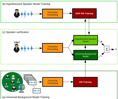
Figure 3.1 shows an expanded GMM-UBM verification system, with the non-hypothesised (a), and hypothesised (b) pre-training model stages included. The diagram illustrates how Reynolds

et al [16] represents the non-hypothesised speaker model by a single large universal background model. The main alternative approach according to Reynolds et al [16] at the time, was oth-erwise to train a collection of individual non-hypothesised speakers, specific for each speaker.

Figure 3.1: Likelihood-ratio based speaker verification system using a single reference universal background model (UBM). The first stage to training a GMM-UBM ASV, is to (a) train a UBM on a extremely last cohort of background speakers, enabling then, (b) hypothsised speaker models to be then trained using MAP adapted EM training, relative to the central reference UBM. With both the non-hypothesised UBM and hypothesised speaker models trained, likelihood-ratio based speaker verification (c) can then be applied to unknown speech recordings, with yes/no decisions made using a pre-defined score decision threshold.

However for applications requiring a large number of hypothesised speakers, preparing individual background sets for each speaker is far from practicable [29].

Figure 3.1 illustrates how the first stage to training a GMM-UBM system, is to (a) train the UBM against a large cohort of background speakers. This is implemented usually with the expectation maximisation (EM) algorithm, with the amount of background speech material used often vast. For telephony conditions, this often involves multiple NIST-SRE evaluation and Switchboard corpora [3], equating to thousands of hours of speech data.

Once a UBM has been successfully trained, it is then used in the maximum a-posteriori (MAP) adapted EM training of hypothesised speaker models (b). The final non-hypothesised UBM and the hypothesised speaker models, can then be used to perform likelihood ratio-based speaker verification on unknown speech recordings (c), as defined previous by Equation 2.1.

Interestingly, the use of a single large background model was also proposed by Careyet al[30] at a similar time, which they referred to as a ‘General Model’. The difference with their work is that they proposed instead a text dependent hidden Markov model (HMM) speech recogniser, fed into a form of recurrent neural network to make decisions. According to Auckenthaler et al[31] however, subsequent work by Parris et al [32] investigating discrimination of phonemes for text independent verification applications, was found not to perform as well as GMM-UBM based equivalents. Auckenthaler et al concluded in [31] that this was most likely due to the training data not being able to be shared between the Gaussian mixture components, in comparison to GMM-UBM systems. With the HMM, the data is aligned to the phonetic classes, and consequently no data is then able to be shared between the classes, leading to poorly trained distribution model parameters.

The purpose of this chapter, is to primarily review the early pioneering works in data-driven GMM-UBMs by Reynolds et al [16] during the mid-’90s. This chapter is structured, present-ing each of the main processpresent-ing stages in order of processpresent-ing, beginnpresent-ing with the ‘Front-End Processing’ on feature extraction. This is then followed with the UBM, how it is effectively a large GMM-trained using the EM algorithm, and then the MAP adapted EM training of the hypothesised speaker models. The chapter then concludes with briefly reviewing normalisation techniques commonly applied to the output log-likelihood ratio scores. Research has found that setting the verification decision threshold can be quite troublesome [29], with a number of score normalisation proposed.

3.1

Front End Processing (Feature Extraction)

Feature extraction is a critical first stage in an ASV system, transforming the raw speech signal into vectors that elicit speaker specific characteristics, as well as removing redundancy. Nearly all ASV systems proposed compute cepstral features [15, 16, 29], first proposed by Davis and Mermelstein [33] for ASR, and then applied to speaker recognition by Furui [11].

Figure 3.2 shows the typical cepstral feature extraction process.

Figure 3.2: Cepstral feature extraction process.

Eight processing stages can be seen, through from the underlying audio signal to the final set of feature vectors X.

(1) Pre-emphasis: The first stage is pre-emphasis, which is the appliance of a filter to enhance the higher frequencies of the spectrum, defined in [29] as:

xp(t) =x(t)−a·x(t−1) (3.1)

where ais usually between [0.95, 0.98].

Pre-emphasis is not always applied (illustrated here by the dashed line), the choice being em-pirically defined on a case by case basis [29]. In this work, pre-emphasis has not been explored.

(2) Windowing: Speech signals are rapidly varying time signals, and as such in the second stage, they are split into short-time frame windows [29]. A hamming or hanning window is then

applied to each window, tapering the speech signal to reduce side effects. The window size used here throughout is 32ms, intentionally chosen to be a power of two, with 256 samples at 8kHz sampling frequency for the next Fourier transform stage. The increment is 16ms giving 50% overlap.

(3) VAD: Voice activity detection is required to remove non-speech and silence time frames, that would otherwise lead to degraded speaker verification decisions. In noisy conditions, the robustness of the VAD is likely to be critical to achieving good performance, with it acting as a filter quite early into the process.

(4) |DFT|: The Fourier transform is next applied and its modulus taken, giving an estimate of the power spectrum.

(5) Filterbank: The power spectrum is then multiplied through a filterbank, which comprises a series of bandpass filters often triangular shaped, and spaced either linearly or perceptually according to the Bark/Mel scale [29].

The Mel scale is given by the equation below, and is said to reflect human perception of pitch:

fM el = 1000·

log(1 +fLIN/1000)

log2 (3.2)

The filterbank used here is Mel spaced with nominally 26 triangular filters, but a more appro-priate number for future research on telephony band-limited speech is possibly around 20 [34].

(6) Log: The logarithm of the filterbank outputs is then taken, to better reflect human percep-tion of loudness. It is likely also applied to compensate for the natural downwards tilt of the magnitude spectra with frequency.

(7) DCT: To then transform into the cepstral domain, the discrete cosine transform (DCT) is taken. This effectively is a decorrelation on top of the Fourier transform, and a dimension

reduction. Typically a higher order of 19 coefficients is retained [3, 12].

(7) Centre & Reduce: The cepstral coefficients are then centralised to the mean on a recording basis, which is found from a practical experience here to be critically important for achieving good performance. Early work by Reynolds in [35] showed that cepstral mean subtraction gave a 25% percentage increase in performance, removing potential convolutional noise. He also compared Rasta filtering as alternate process, finding that whilst this helped, it was no better if not worse than cepstral mean removal. The cepstra is also sometimes then “reduced” or variance normalised [29]. Cepstral mean subraction with variance normalisation (CMV) is applied here.

3.2

Dynamic Feature Extraction

In order to try and incorporate dynamic time varying information into the models, delta and double delta cepstra are normally computed. They are usually calculated as a polynomial approximation, spanning a finite duration either side to the current feature vector.

The defining equations taken from [29] are as follows

δcf(t) δt ≈∆cf = Pl k=−lk·cf+k Pl k=−l|k| δ2_c f(t) δ2_t ≈∆∆cf = Pl k=−lk2·cf+k Pl k=−lk2 (3.3)

wherekdefines the time frame andf the cepstral feature order. Both Reynolds [16] and Garcia-Romero [12] set l as two frames either side of the current feature vector [16].

The open source Voicebox toolkit created by Brookes [36] used here to extract the cepstral features for all experiments, uses four time frames either side to compute the first order, and

one frame either side for the second order differential.

3.3

The Universal Background Model

The universal background model (UBM) is a large Gaussian mixture model, typically consist-ing of between 512 to 2048 mixture components, and is used to compute the required non-hypothesised speaker likelihood p(X|λ_hyp) defined in Equation 2.2.

Following Reynoldset al[16], a GMM probability density used to estimate a likelihood function, can be defined as the weighted linear combination over M unimodal Gaussian densities

p(X_|λ) = M X

i=1

wipi(X) (3.4)

where the M Gaussian densities pi(X) are defined as

pi(X) = 1 (2π)D/2_|Σi|1/2exp −1₂(X₋µi)0(Σi)−1(X−µi) (3.5)

withwirepresenting the weights (which must satisfy the constraintPMi=1wi = 1, and are strictly non-negative); µi, the mean, being a vector D x 1; and Σi, the D xD covariance matrix. The parameters of a Gaussian mixture model thus are denoted by Reynolds [16] asλ=_{wi, µi,Σi}.

The likelihood model training criterion can then be defined as the cumulative product across all feature vector instances, X =_{x1, ..., xT}:

p(X_|λ) = T Y t=1

where again often the logarithm is taken, giving a summation form: logp(X|λ) = T X t=1 log p(xt|λ) (3.7)

The UBM is trained in practice using the expectation-maximisation (EM) algorithm, which iteratively refines the GMM parameters to locally maximise the likelihood p(X_|λ).

3.4

UBM-MAP Speaker Model Training

The speaker specific models are trained via a Bayesian maximum a-posteriori (MAP) adaptation procedure, relative to the UBM. This procedure was proposed by Reynolds [16], following the original MAP procedure published by Gauvain and Lee [37], and is similar to the EM algorithm, but differs in the maximisation stage.

By defining the speaker models in reference to the UBM, helps to alleviate the small amount of training data usually only available to train the individual models. UBM’s typically are trained with more than 1000 hours of audio [3,12], meaning that they are well defined. Crucially as well, the UBM in effect provides a probabilistic reference, allowing speaker models to be compared. The MAP training also helps to provide a tight coupling between the UBM and the speaker models [29], improving performance.

Figure 3.3 re-drawn from Reynolds [16], helps to illustrate this process, with a fictional two dimensional feature space. The well trained UBM model mixture components can be seen to be adapted dependent on whether there is a high count of speaker specific training data.

Components C1 and C2 for example do have a high amount and are adapted accordingly, but

C3 does not, and is not changed.

Figure 3.3: Illustration of how the speaker model Gaussian components are referenced relative to the universal background model (UBM) via maximum a-posteriori adaptation (MAP). Gaussian components C1 and C2 are opportunely adapted by the speaker enrolment features available, with C3 left defined by the original UBM.

it sets the ground for the current state-of-the-art i-vector [3] presented later. Taking Bayes’ rule:

posterior= prior·likelihood

evidence

P(A_|B) = P(A)·P(B|A)

P(B)

(3.8)

To train a speaker model (λ), Reynolds [16] defines an EM style MAP modified training proce-dure. Taking that xt instead now represents the training features from a hypothesised speaker, it is first aligned with the UBM mixture components:

p(i_|xt) =

wipi(xt)

PM

j wjpj(xt)

(3.9)

wherewi represents the prior weight, for thei’th mixture component spanning 1 toM, and the likelihood probability is calculated by the Gaussian probability density function:

pi(xt) = 1 (2π)D/2_|Σi|1/2exp −1₂(xt−µi)0(Σi)−1(xt−µi) (3.10)

After the initial alignment of the observation vectors xt with the UBM, the sufficient statistics of the the posterior distributionp(i_|xt) are computed:

ni= T X t=1 p(i|xt) Ei(x) = 1 ni T X t=1 p(i_|xt)xt Ei(x2) = 1 ni T X t=1 p(i_|xt)x2t (3.11)

This Reynolds notes is the same as the expectation step of the EM algorithm. However the next stage, where the model parameters are updated to maximise the likelihood is different.

Reynolds [16] adapts the old UBM model mixture component parameters with the new expec-tations, when computing the new model parameters:

ˆ wi= [αwi ni/T+ (1−αwi )wi]γ ˆ µi=αmi Ei(x) + (1−αmi )µi ˆ σ2 i =αviEi(x2) + (1−αiv)(σi2+µ2i)−µˆ2i (3.12)

A scale factor γ is used to ensure that all adapted mixture weights sum to unity.

The adaptation is controlled by the data-dependent mixing coefficient αp_i, p∈ {w, m, v}, and is defined as:

αp_i = ni

ni+rp

(3.13)

whererp _{is a fixed relevance factor for parameterp. As illustrated earlier in Figure 3.3 with the} conceptual two dimensional feature space, Equation 3.13 shows how mixture components with more speaker training data will have a larger α_ip, and as such will be adapted more.

compo-nents. The value used here is 19, following the Microsoft Research (MSR) Identity toolbox [38]. Reynoldset al[16] report that they find relevance factors in the range of 8 to 20 to be insensitive to ASV performance. They decided on a value of 16.

Further to this, according to Bimbot et al [29], it is found that making r model parameter dependent also brings little benefit. It is found as well that typically adapting only the means brings real benefit. This again was empirically shown by Reynolds et alin [16].

The MAP adaptation procedure proposed by Reynolds can be viewed intuitively, as the linear trade-off between the prior (initialised with the UBM), and the likelihood given the speaker specific training features X available:

p(λ_|X)_∝arg max λ

(logp(X_|λ) +logp(λ)) (3.14)

The MAP concept above still in fact forms the foundation of current state-of-the-art i-vectors [2, 3], which are defined on the GMM-UBM ASV.

3.5

Score Normalisation

With the UBM and speaker models trained, GMM-UBM speaker verification can be applied. An unknown segment of speech audio can be processed against a hypothesised speaker model and the UBM, with the difference between the outputted model probability scores computed using Equation 2.2. If the score exceeds a set threshold, then the hypothesised speaker is accepted or otherwise rejected.

Unfortunately research has found setting this decision threshold to be quite troublesome [29]. The models are ultimately modelled on cepstral features, which are in themselves highly sus-ceptible to unwanted variabilities. Some examples of these unwanted variabilities include

• speaker variabilities: mood, emotion, health, and fundamental frequency;

• transmission channel variabilities: CODECs, background noise, and handset;

• and other variabilities: duration, and phonetic content.

According to Bimbot et al[29], score normalisation was thus introduced to try compensate for this unwanted variability, in an attempt to make the setting of the decision threshold speaker-independent. In their journal paper, they make reference to the study by Li and Porter [39], who they write observed large variances in the target speaker score (intra-speaker scores), and impostor scores (inter-speaker scores) during trialling.

From their study, they proposed the use of the impostor score distributions to normalise the outputted speaker model scores respectively:

ˆ

∧λ(X) = ∧λ

(X)₋µλ

σλ

(3.15)

where µλ and σλ are the mean and standard deviation normalisation parameters for speaker model λ, derived from an impostor score distribution.

This formulation led to an extensive amount of score normalisation research, including zero score normalisation (Z-Norm) above, handset normalisation (H-Norm) by Reynolds et al [16], test normalisation (T-Norm) by Auckenthaler et al [40], cellular normalisation by Reynolds for NIST 2002 [29], and combinations.

The issue with unwanted speaker and channel variabilities is still very much a contested topic. In more recent times this has led to techniques such as probabilistic linear discriminant anal-ysis (PLDA) [41, 42] for scoring, which effectively is a factor analanal-ysis implementation. This is discussed in the following chapter, in association with i-vectors [3], which build upon the GMM-UBM work of Reynolds [16].

I-Vectors

The success of adapted Gaussian mixture models (GMMs) by Reynoldset al[16] highlighted the potential of data-driven approaches. Their work and others related [31, 32], spawned in effect the next decade of research into data-driven modelling techniques, culminating with i-vectors in 2010 by Dehaket al [3]. I-vectors have since largely remained as the state-of-the-art, with only in recent years their successful fusion with deep learnt automatic speech recognition [22, 43]. This chapter reviews i-vectors by Dehak et al [3], and works by Kenny et al [2] prior to deep learning.

I-vectors conceptually build upon the maximum a-posteriori (MAP) adaptation of hypothesised speaker models proposed by Reynoldset al[16], with factor analysis. The use of MAP adaptation relative to the UBM helps to mitigate the often limited amounts of hypothesised speaker training material available, by providing a form of model regularisation. The UBM also provides a probabilistic reference allowing speaker models to be better compared.

Equation 4.1 below is taken from [22, 44], and succinctly defines the i-vector, as the maximum a-posteriori (MAP) point estimate of the latent vector w. The t-th observation vector xt is assumed to be generated by the GMM defined:

xt∼ X

c

γctN(µc+Tcw,Σc) (4.1)

wherecrepresents the Gaussian mixture component index;Tcis a matrix representing a low-rank subspace known, known as the total variability subspace from which the means of each Gaussian are adapted to a speech recording; w is a normal-distributed latent vector that is recording

specific, and is referred to as an i-vector, µc and Σcare the mean and covariance matrix of the unadapted c-th Gaussian of the speaker population (note that Σc can be updated [2], but in practice this supposedly found to bring little benefit [22]); andγctrepresents the alignment of the observation xt to Gaussian componentcat time t, or weight, and is given byγct=p(c|xt). The weights γct, covariance matrix Σc, and offset mean µc, are derived in practice from a universal backgound model (UBM) [12, 45].

Following Garcia-Romero’s description [12], Equation 4.1 illustrates how the means of the GMM are assumed to be random vectors generated by a second stage of generative modelling. A supervector is constructed, by concatenating together all the mixture component means M = [MT

1 , ..., MCT]T, which is assumed to obey the linear model:

M =µ+T w (4.2)

where: M is of dimensionCFx1, withCnumber of mixture components, and feature dimension order F; and that the prior distribution of the mean supervector M is Gaussian, with mean µ

and covarianceT T∗_.

The total variability subspace captures both the desired speaker, and undesired variabilities. The matrix T (CFxKT) defines the mapping from the high dimensional CF supervector space, with the eigenvectors ofT T∗notionally defining theKT principle eigenvectors of the supervector covariance matrix [2]. The dimension of the total variability factors wor i-vector is KTx1.

Prior to i-vectors, Kenny et al [46] proposed the Joint Factor Analysis (JFA) model, where the factor analysis model of the means of each mixture component is expanded to:

M =µ+U x+V y+Dz (4.3)

variability subspaces respectively;x(KU x 1) andy(KVx1) are normal-distributed independent latent vectors representing the speaker and channel dependent factors; and D is a diagonal

CFxCF matrix representing residual variability not captured by the two other components, with z(CFx1) representing the respective normal-distributed latent residual-factors.

JFA approximately halved the percentage equal error rate of GMM-UBM verification based systems, from notionally 8% down to 4% [17]. Dehaket al[3] states that the original motivation to investigate i-vectors, utilising a single total variability subspace, was because he found that the channel factors (x) of the JFA model, in fact contained speaker information. During JFA scoring, Dehaket al[3] describes how the likelihood of a test utterance feature vector is computed against a channel-compensated speaker model (M₋U x), implying thus a potential loss of speaker discriminative information.

It should also be notably mentioned, that performances similar to JFA were also being achieved using nuisance attribute projection (NAP) [47]. The key concept described in [48] behind NAP, is to remove dimensions from a support vector machine (SVM) expansion, which are irrelevant to the speaker recognition task. NAP was developed independently in parallel to JFA.

The intention of this chapter is to review the theory and implementation behind i-vectors. As such, the remainder of this chapter is structured, with first a review of the training process to estimate the total variability matrix (T-matrix), before then summarising the key T-matrix training steps and extraction of i-vectors from speech utterances. The chapter then concludes by reviewing verification procedures, and in particular probabilistic linear discriminant analysis (PLDA) [41] scoring, which has been key to achieving state-of-the-art performance.

4.1

Training the T-Matrix

In this sub-section, the total variability matrix (T-matrix) training procedure is presented.

The T-matrix is trained iteratively, using typically the expectation maximisation (EM) algo-rithm. Dehak et al[3] writes that the same procedure used to estimate the eigenvoice matrix V

in [2], is used. Equation 4.4 is taken from [2], and defines the eigenvoice matrixV within the fa-miliar mean supervector maximum a-posteriori (MAP) model, for speakers; and the unadapted speaker population offset µ, usually defined by a universal background model (UBM).

M(s) =µ+V y(s) (4.4)

The one significant difference with the eigenvoice matrix V Dehak et al [3] writes, is that all the training recordings from the same speaker are considered as belonging to the same speaker. However when training the T-matrix, they pretend that all the training recordings from the same speaker are derived from different speakers. The objective is to estimate the total variability subspace, independent of speakers and channels. For further reference, a useful practical implementation guide is also given by Lei in [45].

Thus following the eigenvoice matrix V training by Kenny et al [2], and substituting V forT; they proposed the likelihood objective function to maximise, similar to Reynolds [16], as

Y s

PT,Σ(X(s)) (4.5)

wherePT ,Σ(X(s)) is the probability of the training observation feature vectorX(s), for speakers,

given the GMM modelλ(s) corresponding to the supervector containingT w(s) with unadapted covariance matrix Σ (note again that Σ can be updated [2], but in practice this is supposedly found to bring little benefit [22]). The probability is then extended across all speakers sby the

taking the product.

The training procedure proposed by Kenny et al [2], can be split into three stages. The first stage is a preparation stage, whilst the second and third correspond to the iterative expectation maximisation (EM) algorithm:

(1) Prepare the required zero’th, first, and second order statistics expanded into matrices.

(2) The expectation step of the EM algorithm: the posterior distribution of the latent i-vector

w(s) (equivalent to y(s) with eigenvoices) is calculated, using the current alignment of speaker s’s feature vector, the current estimate ofT, and the priorN(y_|0, I).

(3) The maximisation step: updateT by a linear regression, using the new posterior distribu-tion estimates of w(s).

Fundamentally the training procedure can be viewed as fitting feature observations to the Gaus-sian component densities, such that the conditional likelihood criterion previous (Eq. 4.5) is maximised. Thus following Kennyet al’s [2] observations, and taking the standard GMM model equation to be maximised X s X c Nc(s)log 1 (2π)F /2_|Σc|1/2 − 1 2 X t (xt−Mc(s))∗Σc−1(xt−Mc(s)) ! (4.6)

where s ranges over all speakers in the training set, c spans all mixture components, and t is summed over all time framesxtaligned withcfor speakers; if the covariance matrix Σ is already estimated, then the problem can be seen to reduce to a least mean squares minimisation exercise of fitting Gaussian densities

X t

(Xt−Mc(s))∗(Xt−Mc(s)) (4.7)

where Σ−1

Unfortunately fitting the Gaussian densities is complicated because the true Gaussian state structure for each speaker sis hidden, and the GMM model parameters are not fully sufficient to explain λ(s) relative to the training observation vectorsX(s).

More practically explained, the Gaussian component densities will have regions of overlap, lead-ing to regions of uncertainty as to how to best fit the trainlead-ing observations, and therefore givlead-ing rise to the presence of latent parameters. This is also further complicated by the use of MAP adaptation, requiring a maximum criterion trade-off between the original model prior parameters values p(λ(s)), and new training data likelihood updates p(X(s)|λ(s)) [16, 37].

To address these difficulties, Kenny et al[2] follow Reynolds et al’s [16] and Gauvain and Lee’s [37] approach, by utilising the EM algorithm to train the T matrix. The EM algorithm is used to iteratively estimate T, such that the likelihood criterion Q_sPT ,Σ(X(s)) accrued across all

training speakerss is maximised.

Kenny et al [2] propose repeatedly estimating in turn the expectation of the latent parameters (i-vectorsw(s)) whilst holding all the model parameters constant, and then subsequently feeding the new latent parameter estimates back in to update the model parameter estimates (the T

matrix). The EM process is repeated until Q_sPT ,Σ(X(s)) converges at a maximum value.

The EM training of the T-matrix is next presented in depth, following the eigenvoiceV matrix training procedure in [2], whilst also remembering that all training recordings are treated as if they were all produced by different speakers instead.

4.1.1 Stage 1 - Prepare Required Statistics

For each training speaker recording, the zero’th, first and second order statistics are required:

Nc(s) = X t p(c_|xt) Fc(s) =X t (xt−µc) Sc(s) =X t (xt−µc) (xt−µc)∗ (4.8)

where c is the mixture component, s is a speaker recording, t is the time frame, and µ is the speaker independent mean offset, typically defined by a pre-trained UBM.

Expanding into matrices:

NN(s) =       N1(s)∗I . .. NC(s)∗I       FF(s) =       F1(s) .. . FC(s)       SS(s) =       S1(s) . .. SC(s)      

where NN(s) is the zero’th order diagonal matrix, of dimension CDxCD, with C mixture components and D feature dimension order; FF(s) represents the first order matrix of length

CD, centralised to the speaker independent mean offset (UBM), and I is the identity matrix; and SS(s) represents the second order diagonal matrix of dimension CDxCD.

4.1.2 Stage 2 - Calculate Posterior Expectation ofw(s)(EM Algorithm)

The posterior distribution of the latent vector w(s), is calculated using the current alignment of the speaker s’s training feature dataX, the current estimates of T, and the prior N(y|0,1). On the first iteration T is randomly initialised.

Kenny et al [2] derive the required expectation of w(s) from Bayes’ posterior equation below (dropping the reference to s):

PT(w|X)∝PT(X|w)N(w|0, I) (4.9)

or in notation used so far:

p(w_|X, T)_∝p(X_|w, T)p(w) (4.10)

where p(w_|X, T) represents the current estimate of posterior distribution ofwto be calculated, and T the model parameters to be estimated.

Kenny et al gives a full derivation in Appendix-Proof of Proposition 1 of [2], but essentially solves Eq. 4.9, by presuming the distribution form:

p(w_|X(s), T)_∝exp

−1₂(w₋a(s))∗l(s)(w₋a(s))

(4.11)

where a(s) represents the required posterior mean expectation of the latent vectorw(s), which they define as:

a(s) =l−1_(s)T∗_Σ−1_FF

x(s) (4.12)

and l(s) is the covariance matrix of the posterior of w(s), defined as:

Kenny et al derivea(s) by essentially beginning from Equation 4.9, solving for:

PT(w|X)∝PT(X|w)N(w|0, I) (4.14)

where the reference to swas dropped for ease of notation.

They then define PT(X|w) in Appendix-Lemma 1 as:

log PT,Σ(X(s)|w(s)) =GΣ(s) +HT,Σ(s,w(s)) (4.15)

with G_Σ(s) representing a Gaussian log likelihood function given by expression:

log p(x_|s) =GΣ(s) = C X c=1 Nc(s) TF log 1 (2π)D/2_|Σc|1/2 − 1 2tr Σ −1 c Sc(s) (4.16)

where TF represents the total time frames, and HT,Σ(s,w) containing the required hidden w

terms is defined as:

HT,Σ(s,w) =w∗T∗Σ−1FF(s)−

1 2w

∗

The proof given to derive HT,Σ(s,w) involves multiplying out the exponent terms from log

likelihood distribution p(x_|w(s)). First they define some useful terms, and again drop the reference tos. They letO =T w, whereOcdenotes the c’th block ofO, with each block aDx1 vector in size (D is the feature dimension order), and define the second order statistic centred additionally by Oc:

Sc(Oc) =X t

(xt−µc−Oc) (xt−µc−Oc)∗ (4.18)

The log likelihood distribution p(x_|w) can then be defined using the two newly defined terms as: p(x|w) =X c Nc 1 (2π)D/2_|Σc|1/2 − 1 2tr Σ −1 c Sc(Oc) (4.19)

To derive HT,Σ(s,w), Kenny et al expand out the exponent term as follows (remembering the

second order statistic Sc(s) from Equations 4.8 defined earlier, and Nc accounting for missing required summation over time for (OcOc∗):

Sc(Oc) =Sc−FcO∗c−OcFc∗+NcOcO∗c (4.20)

re-including the trace

tr Σ−_c1Sc(Oc)=tr Σ−_c1Sc

−2FcΣ−_c1Oc+O∗cΣ −1

c NcOc (4.21)

where the trace of Σ−1

c Scis only required because the matrices in practice are diagonal; the two

FcO∗c andOcFc∗ terms can be grouped because they are equal scalars when multiplied out; and

O∗_cΣ−1

Summing across all Gaussian mixture components leads to the final proof of HT,Σ(s,w), with X c tr Σ−_c1Sc corresponding toGΣ(s): X c tr Σ1_cSc(Oc)=X c tr Σ−_c1Sc −2O∗Σ−1FF +O∗NNΣ−1O (4.22)

Having derived HT,Σ(s,w) containing the pertinent latent vector w terms, Kenny et al

sub-stitutes back into their required Bayesian posterior distribution definition for w (dropping the reference to s): PT(w|X)∝PT(X|w)N(w|0, I) ∝exp w∗T∗Σ−1FF ₋1 2w ∗_T∗_NNΣ−1_{T w−}1 2w ∗_w ∝exp w∗T∗Σ−1F − 1 2w ∗ T∗NΣ−1T +Iw =exp w∗T∗Σ−1F −1 2w ∗ lw ∝exp −1₂(w₋a)∗l(w₋a)

By assuming that the posterior distributionpT(w|X) must be of a Gaussian form, they solve to find the required posterior mean value a, given covariance matrixl−1_:

a(s) =l−1(s)T∗Σ−1FF(s) (4.23)

The original mean MAP adapted i-vector equation (Eq. 4.2), can thus be expanded to its full form:

M(s) =T w(s) +m

ˆ

M(s) =T l−1(s)T∗Σ−1FFX(s) +m

4.1.3 Stage 3 - Update T via Maximisation (EM Algorithm)

The T matrix is next updated by a linear regression procedure, where the hidden variablew(s) now plays the role of an explanatory variable. Kennyet algives a very lengthy derivation in the Appendix of [2], under Proof of Proposition 3.

Kenny et al otherwise defines the new estimates ofT (and Σ), as the solution of: X

s

(NN(s)T E[w(s)w∗(s)]) =X s

(FF(s)E[w∗(s)]) (4.25)

wheresrepresents each training speaker (remembering for T-matrices, different recordings from the same speaker are treated as if they were produced by a different speaker); andE[w(s)], and

E[w(s)w∗_{(s)] are the first and second order moments ofw(s), calculated from the new posterior} distribution expectation estimates.

To solve Equation 4.25, Kenny et alfirst note that NN(s) is diagonal, and equate the ith row of the left hand side to the ith row of the right, for i= 1, ..., CD (where C is the total number of components, andD the feature dimension order). This gives

TiX s

NNi_(s)E[w(s)w∗_(s)]=X s

FFi_(s)E[w∗_{(s)] (4.26)}

where Ti _{is the ith row ofT, and similarly for NN}i_{(s) and FF}i_(s).

They then go further, by making the observation that the zero’th order (diagonal) matrixNN(s) values are the same, for each respective Gaussian mixture component. Letting i then be of the form (c−1)D+d, where 1≤c≤C and 1≤d≤D, then NNi_{(s) =Nc(s), gives}

TiX s (NNc(s)E[w(s)w∗(s)]) = X s FFi(s)E[w∗(s)] (4.27)

T is then solution of a (KTxKT) system of equations, where each row Ti is calculated inde-pendently in turn, and NNc is effectively a scalar value for each Gaussian mixture component. First re-arranging for clarity, and noting that the bracketed left terms multiply out to a scalar

allowing _" X s (NNc(s)E[w(s)w∗(s)]) # Ti =X s FFi(s)E[w∗(s)] (4.28)

The solution for T then is

Ti ₌ X s (NNc(s)E[w(s)w∗(s)]) !−1 ∗ X s FFi_(s)E[w∗_(s)] ! (4.29) whereE[w∗_{(s)] = l}−1_(s)T∗_Σ−1_FF X(s) ∗

, and E[w(s)w∗_{(s)] =l}−1_{(s), which can be calculated}

The proofof the system equation 4.25 is defined in the Appendix of [2] underProof of Proposition 3, and involves constructing an EM auxiliary function, with w as the hidden variable. The theoretical construct involving Jensen’s inequality is first reviewed, before then following the derivation given Kenny et al [2].

Following the EM tutorials by Andrzejewski [49], Mackey [50], and Ng [51], the objective is to maximise the likelihood of the observed data xgiven model parameters λ. Letting w represent a latent variable, then the conditional log likelihood can be defined as (dropping the reference tos): log(p(X|λ)) =log X w p(X, w|λ) ! (4.30)

Defining then some auxiliary distributionq(w) for w, this leads to

log(p(X|λ)) =log X w q(w)p(X, w|λ) q(w) ! (4.31)

A lower likelihood is then formalised using Jensen’s inequality for a concave function, given that it is not possible to directly maximise p(X_|λ) due to the latent model variable w

f(E[X])≥E[f(X)] (4.32)

which then substituting Equation 4.31 into Jensen’s inequality

log(p(X|λ)) =log X w q(w)p(X, w|λ) q(w) ! ≥Ew∼q log p(X, w|λ) q(w) ≥X w q(w)log p(X, w_|λ) q(w) ≥X w q(w)log(p(X, w_|λ))₋X w q(w)log(q(w))

Thus the following observation can be drawn

log(p(X|λ))≥ Ew∼q[log(p(X, w|λ))]

| {z }

Expected Complete Log−Likelihood

+Ew∼q[log(q(w))]

| {z }

Entropy H(w)

=A(w, λ) (4.33)

where the lower defined limit comprises of the expected complete log-likelihood, with respect to

w drawn from distributionq; and the entropy or uncertainty H(w) of latent variable w. This lower bound is typically referred to as an auxiliary function, defined here as A(w, λ).

The EM algorithm in its general form is precisely then coordinate ascent on the two variables

w and λ, of the log-likelihood lower bound A(w, λ) [50]

(1) E-Step: q(i+1)_{(w) =argmax}

qA(w, λi) (2) M-Step: λi+1 _=argmax

λA(w(i+1), λ))

where irepresents the iteration number.

The M-Step is thus the maximisation of the auxiliary function A(w, λ), defined by Equation 4.33 with respect to parametersλ. This maximisation is equivalent to maximising the expected complete log-likelihood (ECLL) under q, provided the entropy or uncertainty H(w) can be minimised.

The expectation E-Step is used to derive an optimal value for q(w), which the solution is

This solution for q(w) can be derived as follows log(p(X|λ))≥Ew∼q log p(X, w|λ) q(w) ≥Ew∼q log p(w_|X, λ)p(X_|λ) q(w) ≥log(p(X_|λ))₋Ew∼q log q(w) p(w|X, λ ≥log(p(X|λ))−KL p(w|X, λ) q(w) (4.35) ≥log(p(X|λ))−KL p(w|X, λ) p(w_|X, λ) ≥log(p(X_|λ))

The solution then forq(w) involves minimising the Kullback-Leibler (KL) divergence, by setting

q(w) =p(w|X, λ). Substituting this solution for q(w) leads to inequality becoming an equality. Given that the log-likelihood provides an upper limit for the auxiliary function for allq(w), the equality result indicates that choice of q(w) must be maximal.

Finally returning to Kenny et al’s derivation, they first begin by constructing the required Jensen’s inequality for the EM algorithm. Referring to the earlier stated definition equations

f(E[x])≥E[f(x)] ≥X w q(w)(i+1)_log p(w|λ(i), X) q(i+1)_(w) !

and substituting in the required terms gives

f(E[X])≥X s Z logPT ,Σ(X(s), w)) PT0,Σ0(w|X(s)) PT0,Σ0(w|X(s))dw (4.36)

Kennyet althen from this define their required auxiliary function to be maximised, with respect toT.

A=X s

Ew∼q[logPT ,Σ(X(s)|w(s))] (4.37)

The derivation of this can be explained by the KL equality derivation, Equation 4.35 previous, resolving to posterior probably of observation vectorsX given modelλ. This can be re-written in the earlier proof definition format

A=X s

Ew∼q[logP(X(s)|λ(s) ={w(s), T,Σ})]

Kenny et al then refer back to their previous general definition for the logPT ,Σ(X|w(s)) (in

Lemma 1 of the Appendix), displayed previously here in Equation 4.15 as

A=X s GΣ(s) + X s Ew∼q[HT ,Σ(s, w(s))] (4.38)

They first term does not contain any reference toT, and so will be disappear when differentiated with respect to T. Kennyet al thus focus on the second term defined as

X s Ew∼q[HT ,Σ(s, w(s))] = X s Ew∼q w∗(s)T∗Σ−1FF(s)₋1 2w ∗ (s)T∗NN(s)Σ−1T w(s) (4.39)

resolving to a more suitable form for matrix differentiation, beginning with the second term

=X s Ew∼q[w∗(s)]T∗Σ−1FF(s) − 1 2tr T ∗_NN(s)Σ−1_{T E} w∼q[w(s)w∗(s)] (4.40)

since 1₂w∗(s)Bw(s) = ₂1tr(w∗(s)Bw(s)) holds true because the end result is a scalar, where B

represents hereT∗NN(s)Σ−1_{T, andw(s) importantly is a vector. This is then further translated}

to 1 2tr(w

∗_{(s)Bw(s)) =} 1

2tr([Bw(s)]w

summa-tion (property: tr(XY) =tr(Y X), whereXis anxmmatrix, andY is amxnmatrix). Kenny

et althen re-write the expectation within the second term, since both the trace and expectation are linear operators.

Next they re-write the first term to required differential form, whilst also factorising out the expectation and Σ, and changing slightly the ordering of the second term (again the property: tr(XY) =tr(Y X)), giving the required form for differentiation

=X s tr Σ−1 FF(s)Ew∼q[w∗(s)]T∗− 1 2NN(s)T Ew∼q[w(s)w ∗_(s)]T∗ (4.41)

where the first term follows from

Ew∼q w∗(s)T∗Σ−1_{FF(s)=tr E} w∼q w∗(s)T∗Σ−1_FF(s) =tr [E[w∗(s)]T∗]Σ−1FF(s) =tr Σ−1FF(s)[Ew∼q[w∗(s)]T∗] =tr Σ−1_(FF(s)E w∼q[w∗(s)]T∗)

Kenny then differentiates Equation 4.41 with respect to T, setting the gradient to 0, to obtain the required system of normal equations (Equation 4.25 previous), which can be solved for the update of T.

Taking the matrix differentiation identities

δBθ∗ δθ =B

δθBθ∗

δθ =θ(B+B

∗_{) (4.42)}