Image Spam Detection

(1)

San Jose State University

SJSU ScholarWorks

Master's Projects Master's Theses and Graduate Research

Spring 5-21-2017

Image Spam Detection

Aneri Chavda

San Jose State University

Follow this and additional works at:https://scholarworks.sjsu.edu/etd_projects

Part of theArtificial Intelligence and Robotics Commons, and theInformation Security Commons

This Master's Project is brought to you for free and open access by the Master's Theses and Graduate Research at SJSU ScholarWorks. It has been accepted for inclusion in Master's Projects by an authorized administrator of SJSU ScholarWorks. For more information, please contact Recommended Citation

Chavda, Aneri, "Image Spam Detection" (2017).Master's Projects. 543. DOI: https://doi.org/10.31979/etd.myqt-f92r

(2)

Image Spam Detection

A Project Presented to

The Faculty of the Department of Computer Science San José State University

In Partial Fulfillment

of the Requirements for the Degree Master of Science

by Aneri Chavda

(3)

(4)

The Designated Project Committee Approves the Project Titled

Image Spam Detection

by Aneri Chavda

APPROVED FOR THE DEPARTMENT OF COMPUTER SCIENCE

SAN JOSÉ STATE UNIVERSITY

May 2017

Dr. Mark Stamp Department of Computer Science

Dr. Thomas Austin Department of Computer Science

(5)

ABSTRACT

Image Spam Detection by Aneri Chavda

Email is one of the most common forms of digital communication. Spam can be defined as unsolicited bulk email, while image spam includes spam text embedded inside images. Image spam is used by spammers so as to evade text-based spam filters and hence it poses a threat to email based communication. In this research, we analyze image spam detection methods based on various combinations of image processing and machine learning techniques.

(6)

ACKNOWLEDGMENTS

I would like to thank my family and friends who have motivated me and have contributed in shaping my journey. I would like to thank Dr. Mark Stamp for providing constant guidance for my project. Dr. Stamp helped me look at security domain from a different perspective.

My parents, Mr. Girish Chavda and Mrs. Urmi Chavda have been my pillars of strength. They have made me a better person and supported all my endeavors in life. I would like to thank them for believing in me and pushing me further to purse Master's. I would also like to thank my little brother Mr. Jeet Chavda for being there for me and constantly motivating me.

(7)

TABLE OF CONTENTS

CHAPTER

1 Introduction . . . 1

2 Background . . . 3

2.1 Types of Image Spam . . . 3

2.2 Spam Detection Techniques . . . 3

2.3 Related Work . . . 4

3 Image Processing. . . 6

3.1 Image Features . . . 6

3.2 Feature Extraction . . . 9

4 Support Vector Machines (SVM) . . . 11

4.1 SVM Model . . . 11

4.1.1 Training Phase . . . 12

4.1.2 Testing Phase . . . 12

4.2 Feature Selection . . . 13

4.2.1 Recursive Feature Elimination . . . 13

4.2.2 Univariate Feature Selection . . . 14

4.3 Scoring Metrics . . . 14

4.3.1 Confusion Matrix . . . 15

4.3.2 Receiver Operating Characteristic(ROC) Curve . . . 15

5 Challenge Dataset Generation . . . 17

(8)

5.1.1 Dataset 1 . . . 17

5.1.2 Dataset 2 . . . 17

5.2 Challenge Dataset Generation - Method . . . 17

6 Experiments and Results . . . 22

6.1 Environment Setup . . . 22 6.2 Experiments . . . 23 6.2.1 Dataset 1 . . . 26 6.2.2 Dataset 2 . . . 27 6.2.3 Challenge Dataset . . . 29 6.3 Feature Selection . . . 31

6.3.1 Recursive Feature Elimination . . . 33

6.3.2 Univariate Feature Selection . . . 35

6.4 Discussion . . . 37

7 Expectation Maximization Clustering . . . 39

7.1 Experiments . . . 39

7.1.1 EM Clustering with two clusters . . . 39

7.1.2 EM Clustering with multiple clusters . . . 42

8 Conclusion and Future Work . . . 44

LIST OF REFERENCES . . . 45

APPENDIX A Feature value comparison scatter plots for test dataset . . . 48 B Feature Weight Comparison for Dataset 1, Dataset 2 and Challenge Dataset 56

(9)

C EM Clustering Results . . . 58

C.1 EM clustering results for 5 clusters . . . 58

(10)

LIST OF TABLES

1 Feature set . . . 10

2 Python Packages . . . 22

3 Dataset 1 - SVM Results . . . 26

4 Dataset 2 - SVM Results . . . 28

5 Test Dataset - SVM Results . . . 29

6 Clustering Scores . . . 41

(11)

LIST OF FIGURES

1 RGB Channels of Color Histogram . . . 7

2 HSV Channels of HSV Histogram . . . 8

3 Canny Edge . . . 9

4 Separating Hyper-plane . . . 12

5 Confusion Matrix . . . 15

6 ROC Curve . . . 16

7 Challenge dataset example - Approach 1 . . . 18

8 Challenge dataset example - Approach 2 . . . 19

9 Feature value comparison scatter plots . . . 20

10 Difference between feature ranks for Dataset 1 and Challenge Dataset 21 11 SVM Detection Model . . . 24

12 AUC for individual features . . . 25

13 Dataset 1 - Linear Kernel . . . 26

14 Dataset 1 - RBF Kernel . . . 27

15 Dataset 1 - Polynomial Kernel . . . 27

16 Dataset 2 - Linear Kernel . . . 28

17 Dataset 2 - RBF Kernel . . . 28

18 Dataset 2 - Polynomial Kernel . . . 29

19 Challenge Dataset - Linear Kernel . . . 30

20 Challenge Dataset - RBF Kernel . . . 30

(12)

22 Feature Weight Comparison for Dataset 1, Dataset 2 and Test Dataset 32

23 RFE - Dataset 1 . . . 33

24 RFE - Dataset 2 . . . 34

25 RFE - Test Dataset . . . 35

26 UFS - Dataset 1 . . . 36

27 UFS - Dataset 2 . . . 36

28 UFS - Test Dataset . . . 37

29 EM clustering results for 2 clusters . . . 40

30 EM clustering results for 2 clusters on Combined Dataset . . . 42

31 Purity Scores for increasing clusters . . . 43

A.32 Height . . . 48

A.33 Width . . . 48

A.34 Aspect Ratio . . . 48

A.35 Compression Ratio . . . 48

A.36 File Size . . . 49

A.37 Image Area . . . 49

A.38 Entropy of color histograms . . . 49

A.39 Red channel mean . . . 49

A.40 Green channel mean . . . 49

A.41 Blue channel mean . . . 49

A.42 Red channel Skew . . . 50

A.43 Green channel skew . . . 50

(13)

A.45 Red channel Variance . . . 50

A.46 Green channel Variance . . . 50

A.47 Blue channel Variance . . . 50

A.48 Red channel Kurtosis . . . 51

A.49 Green channel Kurtosis . . . 51

A.50 Blue channel Kurtosis . . . 52

A.51 Entropy of HSV . . . 52

A.52 Hue channel mean . . . 52

A.53 Saturation channel mean . . . 52

A.54 Intensity channel mean . . . 53

A.55 Hue channel Skew . . . 53

A.56 Saturation channel Skew . . . 53

A.57 Intensity channel skew . . . 53

A.58 Hue channel Variance . . . 53

A.59 Saturation channel Variance . . . 53

A.60 Intensity channel Variance . . . 54

A.61 Hue channel Kurtosis . . . 54

A.62 Saturation channel Kurtosis . . . 54

A.63 Intensity channel Kurtosis . . . 54

A.64 Entropy of Local Binary Pattern . . . 54

A.65 Entropy of Histogram Of Gradients . . . 54

A.66 Edge Count . . . 55

(14)

A.68 Signal to Noise Ratio . . . 55

A.69 Entropy of Noise . . . 55

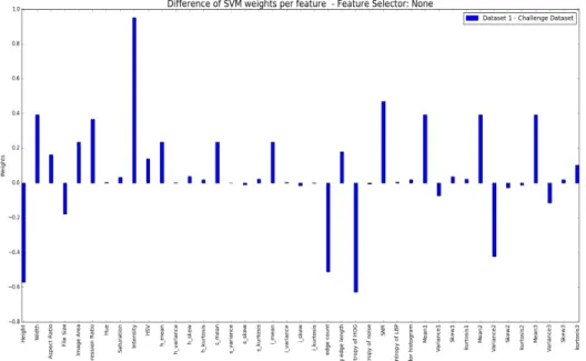
B.70 Feature selector - None . . . 56

B.71 Feature selector - RFE . . . 57

B.72 Feature selector - Univariate Feature Selection . . . 57

C.73 EM clustering results for 5 clusters: Dataset 1 . . . 58

C.75 EM clustering results for 5 clusters: Challenge Dataset . . . 59

C.76 EM clustering results for 5 clusters: Combined Dataset . . . 60

(15)

CHAPTER 1 Introduction

Electronic mail or email is one of the most common forms of digital communication today. A survey conducted in 2010 indicated that 94% of the respondents had used email and 62% used emails daily. These numbers have significantly grown since 2010 [1].

Spam can be defined as unsolicited bulk email. The widespread use of email makes it an attractive target for spammers. Spam email which can include advertisements, malware, phishing links, adult content, and so on, represents a significant threat to the utility of email as a communication medium.

In its nascent stages, spam was seen in the form of text emails. Many strong classifiers were developed to filter spam emails, based on content, subject, header, etc. For example, Lai and Tsai [2] explore 4 machine learning algorithms used to build detection schemes using different parts of the email message. Machine learning

algorithms including 𝑘-nearest neighbors (KNN), Support Vector Machines (SVM),

Naïve Bayes, etc. were used for spam detection.

With strong text based classifiers being developed, spammers reacted by devel-oping new techniques including blank spam, image spam, and backscatter spam to evade text based detection. Image spam is email spam sent in the form of images. Spam text embedded inside an image can be an effective method to evade text-based detection [3]. According to a recent report from Symantec [4], spam now accounts for 90.4% of all email.

Initially, image spam was seen in the form of simple text converted to images. To detect this type of image spam, Optical Character Recognition (OCR) was used. Optical Character Recognition extracts the text inside these images and then it is subjected to text based detection techniques. As a reaction to OCR based detection,

(16)

spammers introduced obfuscation techniques in spam images. Obfuscation prevents OCR from reading the text embedded inside the images [5].

Instead of detecting image spam based on OCR techniques, it is possible to consider a more direct approach based on properties of the images themselves. In this research, we consider such an image processing approach in conjunction with machine learning algorithms.

In addition to our experiments on publicly available image spam datasets, we developed a synthetic dataset. The aim of constructing this dataset was to provide a more challenge test case for proposed detection schemes.

The remainder of this paper is organized as follows. In Chapter 2, we give a brief overview about what is image spam, detection techniques and related work done in this domain. In Chapter 3, we talk about image features used in the experiments. Chapter 4 give a brief overview machine learning model used for the experiments. Chapter 5 we discuss the process of generating the synthetic dataset and evaluate it. Chapter 6 details the environmental setup and then dives into the experimental results of SVM Model with the datasets. We further analyze the feature distribution between ham and spam images with Expectation Maximization Clustering in chapter 7. In chapter 8 we conclude our findings of this research and talk about some future work

(17)

CHAPTER 2 Background 2.1 Types of Image Spam

Image Spam is an email spam technique developed to evade content based detection techniques. Image spam techniques have evolved today. We can loosely classify them into 3 generations [6].

• First Generation Image Spam: The onset of image spam began with simple text embedded inside images. This was a successful effort to evade content based detection schemes. Combining OCR technique with content based filtering served as a good classifier for this class of image spam.

• Second Generation Image Spam: In the second generation of image spam, background images and noise were introduced in the image. This was an attempt make OCR filtering difficult. Since OCR is looking for text inside the images,adding background noise made it difficult for OCR to detect the text. • Third Generation Image Spam: This class of image spam introduced relevant

images along with the text. For instance adding an image of a watch along with the advertisement text. In this scenario, even if OCR detects the text, having an actual watch in the image would confuse the detection scheme.

2.2 Spam Detection Techniques

Spam detection techniques can be loosely split into two categories based on the content of the email.

• Content Based Filters: Content based detection schemes can be used to filter text based spam emails. They rely on the content/text inside the spam emails. String classifiers are built using keywords extracted from spam emails, headers, payload, etc. Machine learning techniques have been used exhaustively to build these type of classifiers [1].

(18)

• Non-content based Filters: Non-content based detection schemes are used to detect more advanced forms email spams like image spam. These detection schemes heavily rely on other properties of the emails like image properties.

2.3 Related Work

Since the onset of spam detection, machine learning techniques have been used exhaustively. Image spam has further widened this research area. A combination of image processing and machine learning techniques have resulted in strong image spam detection schemes.

Kumaresan et al. [7] used combination of 10 metadata features and 3 texture features to construct a feature vector for each image. They used SVM for detection and Particle Swarm Optimization(PSO) to improvise on top of the SVM results. PSO improves the results by iteratively going through candidate solutions and moving the particles in search space. PSO works on a very small dataset compared to SVM. The paper presented SVM plus PSO results for various ratios of training data. Using SVM with particle swarm optimization, they achieved an accuracy of 90% on Dredze dataset for 300 training images and 380 test images.

Annapurna et al. [6] constructed a feature set using 21 image properties. Each fea-ture is associated a weight based on how much it contributes to the SVM classification. Based on these weights, they conducted various experiments, with feature selection and feature elimination. These experiments were conducted on 2 datasets [3, 8] and the accuracy achieved with each dataset was 97% and 99%. As compared to [7]; a lot more features were used to contruct the feature set; and hence the accuracy improved by 9% on Dredze dataset. Additionally, a new in-house dataset was constructed to challenge their SVM classifier.

(19)

The authors used Back Propagation Neural Networks(BPNN) for image spam detection. They achieved an accuracy of 92.82% on the Spam Archive dataset [10] with color features. An interesting feature used in this paper was image composition. Image is partitioned in blocks and the blocks representing left, right and center are considered as super blocks. The mean of these super blocks and uniformity of blocks adjacent to the super blocks are used as features. These features combined give an overview of image composition. They achieved an accuracy of 89.32% on the same dataset using only image composition features.

Chowdhury et al. [11] extracted metadata features and visual features and fed it to BPNN. They presented a comparison of 3 machine learning algorithms; Naive Bayes, SVM and BPNN on the same dataset, with the same set of features. The results showed that despite of increased complexity, neural networks achieved greater accuracy than the other two models.

(20)

CHAPTER 3 Image Processing 3.1 Image Features

Image features are analogous to image properties. Spam images are computer generated. They lack the basic color properties and composition of that of a nor-mal/ham image. Hence, image properties of spam images vary a lot from natural/ham images. For instance change in brightness in natural images is very high compared to that of spam images. We used advanced image processing techniques to extract many such properties from images. A total of 41 features were collected, of which 21 are based on previous research [12]. Table 1 gives a brief overview of all the features. These features can be loosely classified in 5 domains.

• Metadata Features: Properties like image size, height, width, aspect ratio, compression ratio, bit depth, image name, etc. are the basic set of properties of an image. A certain anomaly can be seen in computer generated images versus natural images. We used compression ratio, aspect ratio, etc. as 6 metadata features.

• Color Features: Various histograms contain information about image constitu-tion.

– Color Histogram: A color histogram contains information about the usage

of red, green, and blue colors. Normally, in a spam image, very few colors are used compared to natural images. We also quantized RGB histograms and used them for classification. Figure 1 compares the RGB channels of ham and spam images.

– Red, Green, Blue Histograms: Mean, Variance, Skew and Kurtosis of each

of these 3 histograms is calculated. All combined 12 features are extracted from the 3 histograms.

(21)

(a) Ham (b) Spam

Figure 1: RGB Channels of Color Histogram

– Hue, Saturation and Value (HSV) Histogram: HSV Histogram captures

the following 3 aspects of the colors of an image.

∗ Hue: It defines how close the color is to red. Hue is measured between 0 to 1; 0 being red.

∗ Saturation: It defines how pure the color is. Higher values of saturation correspond to deeper/richer colors. White corresponds to 0 saturation. ∗ Intensity/Value: Intensity defines brightness. Higher values of intensity

correspond to white.

– Hue, Saturation, Intensity Histograms: Mean, skew, variance nd kurtosis

of each of these histograms are captured. This adds up to 12 features extracted from the 3 features. Figure 2 compares the HSV channels of ham and spam images.

• Texture Features:

– Local Binary Pattern (LBP) Histogram: This histogram captures

informa-tion about the texture of the image. For each pixel, LBP helps quantify how similar or different each pixel is from its neighboring pixels. Since spam images do not have a real background, LBP captures relatively less

(22)

(a) Ham (b) Spam

Figure 2: HSV Channels of HSV Histogram

information. • Shape Features:

– Histogram of Oriented Gradients: This histogram is commonly used for

object detection. It describes how the intensity of gradients change in the image.

– Edges: Edges mark the change in contrast. Edges highlight boundaries

of features in an image [12]. Figure 3 shows canny edge filter output on a spam image and a ham image. Spam images in general contain a lot of text, resulting in an increased number of edges than ham images. Another observation we can make by looking at the images is that edges in spam images are smaller compared to that in ham images. Number of edges and average edge length have been considered as 2 features.

• Noise Features:

– Entropy of Noise: Amount of noise in a spam image is less than a normal

image. Entropy of noise histogram is measured as a feature.

– Signal to Noise Ratio (SNR): For this paper SNR is the ratio of mean and

(23)

Figure 3: Canny Edge

3.2 Feature Extraction

Once image properties have been extracted, these features have to be quantified. This process can be called as preparing the data. Machine learning algorithms require input in the form of feature vectors, wherein each feature is a number. Hence image features like canny edges, histograms, etc. have to be converted to numbers. Various statistical techniques like entropy of histograms, mean, variance, kurtosis, extracting number of edges from canny edge image, etc. are used. Once feature vectors are constructed, multiple experiments can be conducted to select a subset of features to achieve greater accuracy.

(24)

Table 1: Feature set

Feature Domain Feature Description

Metadata Features

Height Height of the image

Width Width of image

Aspect Ratio Ratio of height and width

Compression Ratio How compressed is image

File Size Size on disk

Image Area Area of image

Color Features

entr-color Entropy of color histogram

r-mean Mean of red channel histogram

g-mean Mean of green channel histogram

b-mean Mean of blue channel histogram

r-skew Skew of red channel histogram

g-skew Skew of green channel histogram

b-skew Skew of blue channel histogram

r-var Variance of red channel histogram

g-var Variance of green channel histogram

b-var Variance of blue channel histogram

r-kurt Kurtosis of red channel histogram

g-kurt Kurtosis of green channel histogram

b-kurt Kurtosis of blue channel histogram

entr-hsv Entropy of HSV histogram

h-mean Mean of hue channel of hsv histogram

s-mean Mean of saturation channel of hsv histogram

v-mean Mean of brightness channel of hsv histogram

h-var Variance of hue channel of hsv histogram

s-var Variance of saturation channel of hsv histogram

v-var Variance of brightness channel of hsv histogram

h-skew Skew of hue channel of hsv histogram

s-skew Skew of saturation channel of hsv histogram

v-skew Skew of brightness channel of hsv histogram

h-kurt Kurtosis of hue channel of hsv histogram

s-kurt Kurtosis of saturation channel of hsv histogram

v-kurt Kurtosis of brightness channel of hsv histogram

Texture Features lbp Entropy of Local Binary Patterns histogram

Shape Features

entr-hog Entropy of histogram of gradients

edges Total number of edges in an image

avg-edge-length Average edge length

Noise Features

snr Signal to Noise Ratio

(25)

CHAPTER 4

Support Vector Machines (SVM) 4.1 SVM Model

SVM is a supervised learning algorithm, generally used for classification. SVM has been exhaustively used in email spam detection [2] and image spam detection [6]. In the training phase SVM constructs a separating hyper-plane. In this section, we give a brief overview of the SVM algorithm.

There are 4 key concepts of SVM algorithm as described by Stamp M., in Machine Learning with Applications in Information Security [13].

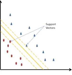
• Separating Hyperplane: In the training phase, SVM attempts to find a separating hyper-plane which divides labeled input data into two classes. In an ideal scenario, all the data of one class falls on one side of the hyperplane and other class falls on the other side.

• Maximize Margins: To construct an optimal hyperplane, only a subset of training data is required. These points are called the support vectors. The idea behind choosing an optimal hyperplane is to maximize the distance/margin between the support vectors of each class and the hyperplane. Figure 4 shows a separating hyperplane and support vectors for 2D data.

• Work in higher dimensions: Separating hyperplane is essentially a linear decision function. However, data of the input space is often not linearly separable. Hence, SVM converts the input data to a feature space higher dimension. Input data in this form is more spread out and linearly separable. Hence, classifying data becomes easier. This transformation is however an expensive task.

• Kernel Trick: Kernel Trick is the mapping function used to transform input space to a linearly separable higher dimension. It makes a non-linear transforma-tion an easy task. It doesn’t actually perform the transformatransforma-tion to the higher

(26)

Figure 4: Separating Hyper-plane

dimension yet gives us the advantages of working in higher dimensions. Multiple Kernel functions are available like Linear Kernel, Polynomial Kernel, Radial Basis Function(RBF), etc.

4.1.1 Training Phase

Training phase involves generating an equation for the separating hyper plane. It is done by solving a Lagrangian Duality problem. Given a set of input data 𝑋0, 𝑋1...., 𝑋𝑛, with labels 𝑧0, 𝑧1...., 𝑧𝑛, where 𝑧𝑖 ∈ {−1,1}, the training phase solves

the Lagrangian Duality Problem for Select Kernal function 𝐾 and 𝐶 as follows

Maximize 𝐿(𝜆) = 1 2 𝑛 ∑︁ 𝑖=1 𝑛 ∑︁ 𝑗=1 𝜆𝑖𝜆𝑗𝑧𝑖𝑧𝑗(𝑋𝑖·𝑋𝑗) Subject to 𝑛 ∑︁ 𝑖=1 𝜆𝑖𝑧𝑖 = 0 and 𝐶≥𝜆𝑖 ≥0 for 𝑖= 1,2. . . 𝑛. 4.1.2 Testing Phase

In the testing phase, we classify a point by determining on which side of the hyperplane the point lies on.

(27)

4.2 Feature Selection

In a multidimensional input space, the cost of converting the input space to a higher dimension increases. Though SVM is a classification algorithm, SVM also calculates weights for each feature and ranks them based on their contribution to classification. The idea behind feature selection is reduction of dimensionality. The cost of converting an input space to higher dimension/applying kernel transformations is high. So instead, using the ranks for each feature, we select only top k features for testing phase. Ranks of each feature indicate the relevance of these features. Some features become redundant in presence of other correlated features. For instance, color histogram and hsv histogram extract different channels of the color properties from an image, hence they are correlated. It could be possible that having color histogram in the feature set alone is sufficient. Hence we use feature selection to cut down this redundancy and increase processing speed. We use two techniques for feature selection described in the following subsections.

4.2.1 Recursive Feature Elimination

Recursive Feature Elimination(RFE)[14] is a statistical feature selection technique, used to remove features that contribute the least to SVM classification. RFE assigns weights to features and ranks them in accordance to the amount of contribution they make towards SVM classification. The feature with least rank is eliminated and the process is repeated till the desired number of features are eliminated. RFE works only with Linear Kernel of SVM.

while 𝑁 𝑜.𝑜𝑓 𝑓 𝑒𝑎𝑡𝑢𝑟𝑒𝑠𝑡𝑜𝑠𝑒𝑙𝑒𝑐𝑡̸=k do

Train SVM classifier.

Calculate weights for each feature and rank them. Eliminate least contributing feature.

(28)

4.2.2 Univariate Feature Selection

Univariate Feature Selection (UFS) [15] uses univariate statistical properties of each individual feature to rank the features. UFS helps understand data structure and characteristics. In contrast to RFE, UFS does not account for feature correlation. This allows UFS to be faster than RFE [16]. The purpose of analyzing this feature selection technique was to contrast RFE selection which is correlation based. UFS uses the coefficients assigned to features by the SVM classifier. This technique is model dependent. When features are highly correlated, model becomes unstable [17].

4.3 Scoring Metrics

When any data point is scored, the result is one of the following 4 outcomes-1. True Positive(TP): The scored sample is a spam, and it is rightly classified as

spam.

2. True Negative(TN): The scored sample is a ham, and it is rightly classified as ham.

3. False Positive(FP): The scored sample is ham, and it is wrongly classified as spam.

4. False Negative(FN): The scored sample is spam, and it is wrongly classified as ham.

In the real world, we want to reduce the FP rate as low as possible and increase TP and TN. We measure SVM scores in the form of accuracy. Accuracy can be defined

as-Accuracy = 𝑇 𝑃 +𝑇 𝑁

𝑃 +𝑁

(29)

4.3.1 Confusion Matrix

Confusion Matrix visualizes the four cases for given dataset. Figure 5 shows a confusion matrix.

Figure 5: Confusion Matrix

4.3.2 Receiver Operating Characteristic(ROC) Curve

For any binary classifier, ROC curve is constructed by plotting True Positive Rate(TPR) versus False Positive Rate(FPR) for varying threshold values. True Positive Rate(TPR) is also called sensitivity, True Negative Rate(TNR) is also called specificity. FPR = 1 - specificity. TPR and TNR can be defined as

follows-TPR= 𝑇 𝑃

𝑇 𝑃 +𝐹 𝑁 and TNR=

𝑇 𝑁

𝑇 𝑁 +𝐹 𝑃

Area Under the Curve(AUC) for an ROC is used as a scoring metric. An AUC of 1.0 is perfect accuracy and AUC of 0.5 is like flipping a coin. “AUC gives the probability that a randomly selected match case scores higher than a non-match case” [18, 13] Figure 6 shows an example of an ROC curve.

(30)

(31)

CHAPTER 5

Challenge Dataset Generation 5.1 Existing Datasets

Two datasets have been used in this research. Two of these datasets are public datasets, images from actual spam and ham emails exchanged.

5.1.1 Dataset 1

This dataset was developed by writers of Image Spam Hunter [3] at Northwestern University. After cleaning the dataset, 920 spam images and 810 ham images were retained for the research. All the images are in jpg/jpeg format.

5.1.2 Dataset 2

Dredze et. al in their paper Learning Fast Classifiers [8], created an image spam corpus which is publicly available. After cleaning the dataset, 1089 spam and 1029 ham images were retained for research. All the images are in jpg/jpeg format.

5.2 Challenge Dataset Generation - Method

The aim of generating this dataset was to challenge the existing detection scheme. Image properties between ham and spam images vary. We used image processing techniques on spam images, to make it look more like a ham image. A public corpus; Spam Archive, from Dredze et. al in their paper Learning Fast Classifiers [8] included only spam images. We used this corpus and overlayed it on the ham images from Dataset 1. The resulting spam images were harder to detect. We used two approaches to develop the challenge dataset. The essential difference between both the approaches was overlay technique.

In approach 1, we attempted to target a set of properties in each step. Steps used to generate challenge dataset using approach 1:

1. We resize the spam images to the image dimensions of a ham image. This will alter the metadata features of spam image, and align them to that of the ham

(32)

images.

2. Since spam images are computer generated, background noise is generally very low in spam images. We added a noise filter to these spam images to introduce some noise in these images. It also masked the sharpness of the edges in spam images.

3. Last step was to overlay this altered spam image to a ham image. We used a weighted overlay technique[]. Weighted overlay technique blends both the images based on the weights specified for each of the image. We experimented with multiple ratios and the ratio that worked best for us was 60% ham and 40% spam.

Figure 7 shows an example of challenge dataset generated using Approach 1. We can see hints of both the images in challenge image. This dataset offsets color, metadata and noise features of the spam image and brings them closer to those of ham images.

Figure 7: Challenge dataset example - Approach 1

(33)

extracted all the content of spam image and overlayed it on ham image. Steps to generate challenge dataset using Approach 2:

1. We resize the spam image to the dimensions of ham image. This resizing helps align the file properties of the test dataset to that of ham set.

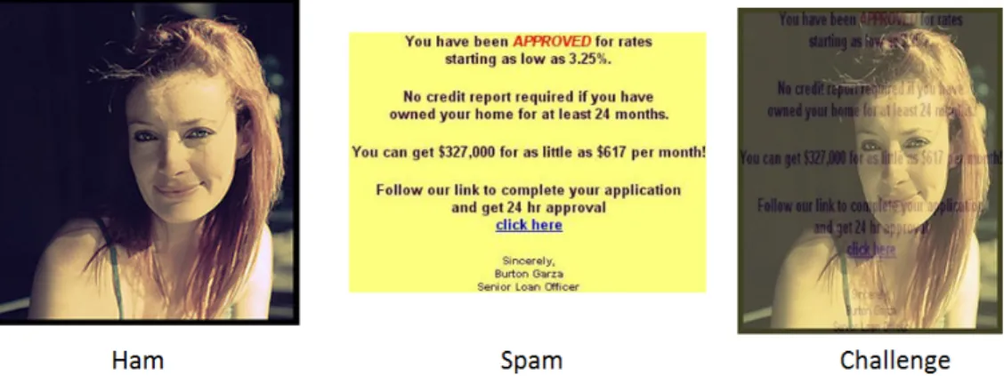
2. We overlay the resized spam images on top of ham images. A general observation we made with the spam images, was that spam images have a light (white/yellow) background. Eliminating the background, we picked up only the content of the spam image and overlaid it on ham image. Doing so, helped us align many image properties like color histogram and edges with that of ham images. Fig. 8. shows an example of the generated dataset. We can see that the test image(generated image), has the ham image as the background and the content of the spam image as the foreground.

Figure 8: Challenge dataset example - Approach 2

Our evaluation criteria for both the approaches was SVM Scores. We subjected these datasets generated by both the approaches to our SVM detection model and approach 1 scored 79% and approach 2 scored 70% accuracy. Since our aim of

(34)

generating these datasets is to challenge the SVM detection model we constructed, approach 2 is clearly better as it brings down the accuracy by 9% as compared to approach 1. All in all, both the datasets give a bigger challenge to the detection schemes and would serve as good challenge datasets for research purposes.

Figure 9 shows scatterplots of compression ratio and color entropy values for ham, spam and test(challenge-spam) images for Approach 2. It can be noted from these scatterplots, that the properties of ham and test image align. Appendix A lists scatter plots of rest of the features. Figure 10 shows the difference in ranks associated to each feature in dataset 1 and challenge dataset. We calculated the ranks per feature for both the datasets and plotted the values of difference between dataset 1 and challenge dataset.

(a) Compression Ratio (b) Entropy of color histogram

(35)

(36)

CHAPTER 6 Experiments and Results

SVM has been widely used in text based detection techniques [1]. In this section we will analyze how SVM can be used in image spam detection. SVM is a supervised classification algorithm. SVM generates a separating hyper-plane at the end of training phase which separates our data into two classes [19]. We use this trained model to test the remaining data.

6.1 Environment Setup

All the experiments were conducted on a Windows 7 Machine with 8 GB RAM and 256 GB SSD. We chose Python as our primary language. Python 3.5.0 with OpenCV [20] were primarily used for all image processing tasks. Scikit-learn library [21] in Python was used for data preprocessing and machine learning tasks. Table 2 lists all the python packages that were used and their purpose.

Table 2: Python Packages

Library Purpose

Open-cv Image Processing for feature extraction

PIL [22] Image Processing for feature extraction

Scikit-learn SVM and preprocessing

Numpy [23] Mathematical computations like mean, var

Matplotlib [24] Charting

Scikit-learn library provides 3 classes for SVM classification - C-Support Vector Classification (SVC), Nu-Support Vector Classification(NuSVC) and Linear Support Vector Classification. SVC internally uses libsvm[25] implementation. SVC is fit for smaller datasets contained within 10000 samples. Since our dataset was a small dataset we used SVC for the experiments. SVC allows multiple kernels of which we used linear, rbf and polynomial. Nu-SVC is nothing but SVC with a specified number of support vectors. Linear SVC is again similar to SVC but does not allow

(37)

kernel selection. Kernel is defaulted to Linear Kernel only. For the experiments we tune various parameters in the SVC method like C, gammma, degree, etc. to achieve optimal results.

OpenCV library is an Open Source Computer Vision library distributed under BSD license. It is widely used in many areas; image processing being one of them. OpenCV library provides interfaces in C, C++, Python, and Java. We used the Python interface of the library. The advantage of using OpenCV against most other image processing libraries was the multitude of features OpenCV came with. Also, since its designed for multi-core processing, we had an added advantage of processing speed.

6.2 Experiments

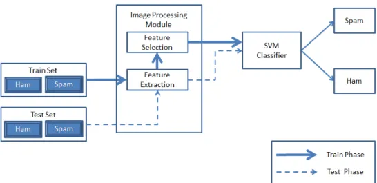
Figure 11 shows the flow of train and test phases for the SVM detection model. First the ham and spam images are split into train and test sets. Train and test sets are exclusive i.e. there is no overlap between the two. All the 41 features are then extracted from the datasets. We then train the SVM classifier with scaled train data. Test set is then passed to the SVM classifier for detection. Additionally, in the train phase, feature selector is added to perform dimensionality reduction based on feature weights.

(38)

Figure 11: SVM Detection Model

To analyze the weight of each feature we calculated SVM scores for each feature individually. Figure 12 shows SVM scores for individual features for all the three datasets. It is easy to note from the three graphs that the SVM AUC scores for individual features for test dataset has gone down significantly compared to those of Dataset 1 and 2.

(39)

(a) Dataset 1 AUC scores for Individual Features

(b) Dataset 2 AUC scores for Individual Features

(c) Test Dataset AUC scores for Individual Features

(40)

6.2.1 Dataset 1

From spam and ham images of dataset 1, we extracted 41 features and scaled them. We used 6% of ham and spam images as training set and rest for testing. A total of 55 spam and 48 ham images were used as train objects. Remaining 865 spam images and 762 ham images were used for testing. Table 3 shows the accuracies and FPR for each of the three SVM kernels. We achieved best results for linear kernel. Figure 13 shows the ROC curve and confusion matrix for linear kernel. Figures 14 and 15 show the results for the kernels rbf and polynomial respectively.

Table 3: Dataset 1 - SVM Results

Kernel Accuracy FPR

Linear 0.97 0.06

RBF 0.96 0.07

Poly 0.95 0.08

(a) ROC Curve (b) Confusion Matrix

(41)

Figure 14: Dataset 1 - RBF Kernel

Figure 15: Dataset 1 - Polynomial Kernel

6.2.2 Dataset 2

All 41 features were extracted and scaled for our dataset. We used 45% of ham and spam images as training set and rest for testing. A total of 490 spam and 463 ham images were used as train objects. Remaining 599 spam images and 566 ham images were used for testing. Table 4 shows the accuracies and FPR for each of the three SVM Kernels. We achieved similar results for linear and rbf kernels. Figures 16,17 and 18 show ROC curve and confusion matrix for all the three kernels.

(42)

Table 4: Dataset 2 - SVM Results

Kernel Accuracy FPR

Linear 0.98 0.02

RBF 0.98 0.02

Poly 0.95 0.10

Figure 16: Dataset 2 - Linear Kernel

(43)

Figure 18: Dataset 2 - Polynomial Kernel

6.2.3 Challenge Dataset

Forty one features were extracted and scaled for images of our in-house generated challenge dataset. We used the dataset we generated with approach 2. We used 30% of ham and spam images as training set and rest for testing. A total of 243 spam and 243 ham images were used as train objects. Remaining 567 spam images and 567 ham images were used for testing. Table 5 shows the accuracies and FPR for each of the three SVM kernels. We achieved best results for Linear Kernel. Figures 19,20 and 21 show ROC curve and confusion matrix for all the three kernels.

Table 5: Test Dataset - SVM Results

Kernel Accuracy FPR

Linear 0.70 0.38

RBF 0.64 0.34

(44)

Figure 19: Challenge Dataset - Linear Kernel

Figure 20: Challenge Dataset - RBF Kernel

(45)

6.3 Feature Selection

Since we have a vast number of features, our next step was to explore techniques to cut down the number of features. Also since we are using image processing to extract these features, feature extraction becomes a computationally intensive task. SVM assigns weights to each of the features it uses. Our initial approach was to rank

these features and elect top 𝑘 features. But, that is not an ideal approach as the

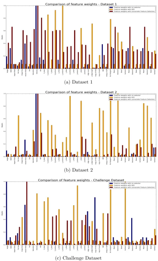
feature weights change per dataset. It can be noted from graphs in Appendix B. We explored two known statistical techniques for features selection - RFE and UFS. Each technique elected a different set of features based on the internal algorithm that they use. It can be noted in the graphs in Figure 22 how feature weights vary based on the feature selection algorithm.

In the following sub-sections we compare and contrast RFE and UFS. From these experiments, it is interesting to note how each algorithm needs a different number of features to gain good accuracy. For our datasets, UFS does a better task at feature selection. UFS requires lesser features to gain the same accuracy as that in RFE. We can see from the graphs in Figure 22 that RFE assigns a lot of weight to multiple features. This can be seen specially in Dataset2 and Challenge Dataset. Appendix B shows graphs for comparison of weight per feature; for all three datasets. For instance, for UFS, we can see the weight of Intensity for Dataset 1 and Dataset 2 is high while for Challenge Dataset it is very low. This is due to the fact that Challenge Dataset successfully altered the color properties of spam images to imitate that of ham images.

(46)

(a) Dataset 1

(b) Dataset 2

(c) Challenge Dataset

(47)

6.3.1 Recursive Feature Elimination

RFE is a feature selection technique used to eliminate features that contribute the least to classification. Here, we use RFE to further tune SVM classification. RFE assigns weights to features and ranks them according to the amount of contribution towards the classification; and eliminates the least ranked features to enhance the accuracy of SVM. RFE algorithm has been discussed in chapter 4.

To gauge how many features are actually needed to achieve maximum accuracy, we

ran SVM with RFE with no-of-features-to-select ranging from 1 to 41. For each value

of no-of-features-to-select, we note down the SVM scores. The following subsection shows the results of this experiment on all the 3 datasets. We used scikit-learn library function rfe for these experiments.

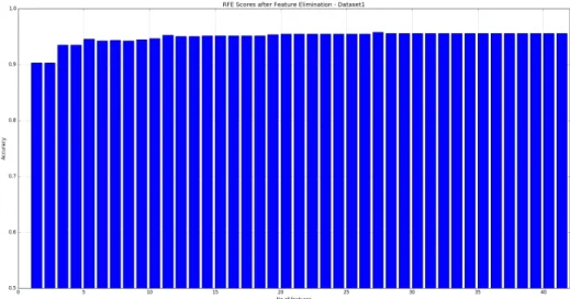
6.3.1.1 Dataset 1

Figure 23 shows RFE results for Dataset 1. We can see from the graph that we achieved maximum 95.57% accuracy after eliminating 13 features.

(48)

6.3.1.2 Dataset 2

Figure 24 shows RFE results for Dataset 2. We can see from the graph that we achieved maximum 98.02% accuracy with only 16 features. Note that as compared to dataset 1, dataset 2 requires less number of features for classification.

Figure 24: RFE - Dataset 2

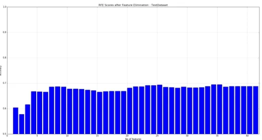
6.3.1.3 Challenge Dataset

Figure 25 shows RFE results for Test Dataset. We can see from the graph that we achieved maximum 69.32% accuracy with 26 features.

(49)

Figure 25: RFE - Test Dataset

6.3.2 Univariate Feature Selection

UFS works differently as compared to RFE. It does not iterate multiple times through the feature set to select the top k features. Instead it performs statistical calculations on features individually and ranks them all at once. Like discussed UFS does not consider the correlation between the features. This allows UFS to be faster.

UFS requires a model as an input. Since, like RFE, we are not bound to one kernel(linear), we used SVM classifier with rbf kernel as an input model to UFS. We used scikit-learn library to implement UFS. We used the method selectKBest along with f-classif classifier which internally uses F-Test. F-Test determines linear dependency of the scaled features. Like RFE, we conducted similar set of experiments on the 3 Datasets with UFS. Following sections show the results of each dataset.

6.3.2.1 Dataset 1

Figure 26 shows UFS results for Dataset 1. We can see from the graph that we achieved maximum 95.15% accuracy with just 1 feature.

(50)

Figure 26: UFS - Dataset 1

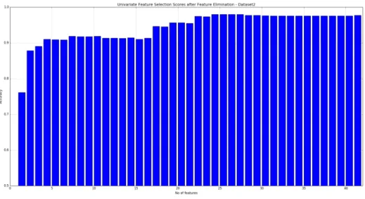
6.3.2.2 Dataset 2

Figure 27 shows UFS results for Dataset 2. We can see from the graph that we achieved maximum 97.93% accuracy with 24 features.

(51)

6.3.2.3 Challenge Dataset

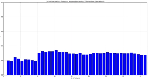
Figure 28 shows UFS results for Test Dataset. We can see from the graph that we achieved maximum 67.07% accuracy with 15 features.

Figure 28: UFS - Test Dataset

6.4 Discussion

In summary, we conducted 2 set of experiments with SVM and Image Processing. In the first set, we considered all the 41 features we extracted from the images. We achieved a good accuracy of 97% and 98% with public datasets Dataset 1 and Dataset 2 respectively. However, with our challenge dataset, the accuracy took a dip to 70%. Which implies we have successfully weakened the system we developed.

In the next set of experiments, we tried to reduce the number of features used in this experiment. We explored 2 different feature selection algorithms - RFE and UFS. We began with comparing and contrasting the weights associated to each of the feature based on feature selection algorithm. In this comparison we could make out that RFE was assigning a lot of weight to multiple features. Hence a solution of SVM with RFE would require more features than that with UFS. We verified this by

(52)

running an experiments to find out optimal number of features required to achieve maximum accuracy. For instance, for Challenge dataset, RFE took 26 features to gain maximum accuracy while UFS needed only 15.

(53)

CHAPTER 7

Expectation Maximization Clustering

Clustering is an unsupervised machine learning technique. The basic idea behind clustering is to form clusters of data, based on some "distance" measurement. Based on this distance measurement, each data point is labeled; where labels describe which cluster the data point belongs to. Expectation Maximization(EM) Clustering algorithm uses probability distributions to label data. EM Clustering algorithm is a 2 step iterative hill climb process [13]

-1. Expectation Step: Recompute the probabilities for each datapoint, that are required in the M step.

2. Maximization Step: Recompute the crucial parameters of the probability distributions.

We used Purity as our scoring parameter for clustering based experiments. Purity measures how clean the clusters are. Its value ranges between 0 to 1. Clusters with multiple classes should have purity value nearing 0, while perfect clustering will have purity value of 1.

7.1 Experiments

7.1.1 EM Clustering with two clusters

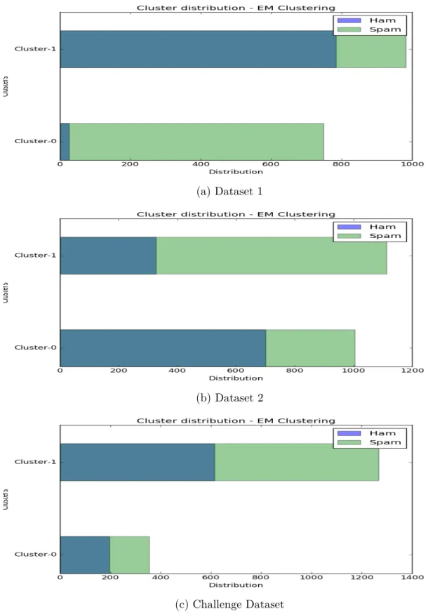
To analyze how the ham and spam cluster, we subjected the 41 image features that we extracted, to EM clustering. In an ideal scenario, with 2 clusters, we would expect all ham images to fall in one cluster and all spam images in another cluster. Figure 29 shows EM clustering results for 3 datasets, using gaussian mixture function from scikit-learn library, with full clustering method.

(54)

(a) Dataset 1

(b) Dataset 2

(c) Challenge Dataset

(55)

Table 6 shows the various scores for all the experiments. For Dataset 1, the cluster have a dominating class for each cluster. All the clustering scores for Dataset 1 are also high compared to the other 2 clusters. Dataset 2 also has a dominating class in each cluster, but the proportions of non-dominating class is higher. Challenge dataset however forms very poor clusters. It only highlights the fact that spam set in challenge dataset is very similar to ham set, and hence, it is difficult to distinguish between the two. We can see the decline in scores from Dataset 1 to Challenge Dataset.

Table 6: Clustering Scores

Dataset Purity Folkes Mallows Homogeneity Completeness V-Measure

Dataset 1 0.87 0.77 0.49 0.49 0.49

Dataset 2 0.70 0.58 0.12 0.12 0.12

Challenge Dataset 0.52 0.57 0.002 0.003 0.002

Combined Datasets 0.62 0.57 0.43 0.40 0.41

In the next set of experiments, we combined Dataset 1 and Challenge Dataset and subjected them to EM clustering. Since we have 3 different labels, we changed the number of clusters to 3. Figure 30 shows the cluster distributions for this experiment. Table 7 shows the number of ham, spam and challenge images in each cluster. We can see from the table that cluster 1 has only spam images. The interesting thing to note in this cluster distribution is that cluster 2 is a combination of challenge and ham images only. We generated the challenge spam set such that it looks more like ham set, and cluster 2 distribution verifies that.

(56)

Figure 30: EM clustering results for 2 clusters on Combined Dataset

Table 7: Cluster Distribution

Cluster Ham Spam Challenge

Cluster 1 7 577 4

Cluster 2 606 0 648

Cluster 3 197 343 158

7.1.2 EM Clustering with multiple clusters

We further subjected our datasets to EM clustering with more clusters than the number of labels. We analyzed the purity score for each of these and saw a rise in the purity of clusters as the number of clusters are increased. But, the difference between the scores between datasets, remains constant. Figure 31 shows purity scores versus number of clusters for all 3 datasets and combined dataset. Appendix C shows the cluster distributions for 5, 10, 15 and 20 clusters respectively.

(57)

Figure 31: Purity Scores for increasing clusters

EM Clustering gave us an insight to what our feature distributions are like. Even though the clusters are not perfect, with our rich feature set of image properties, we got decent results with Dataset 1 and Dataset 2.

(58)

CHAPTER 8

Conclusion and Future Work

With improved spamming techniques, spammers have been successful in evading traditional spam detection techniques like content-based detection and OCR. This opened a door for techniques like image processing to detect image spam. A combi-nation of machine learning algorithms and image processing can be used to constuct strong classifiers. We developed a similar classifier using SVM with image properties as our feature set, which provided good results in image spam detection on two public datasets.

Due to lack of public datasets for image spam research, we explored techniques for constructing new datasets. We successfully constructed a dataset that weakened the detection scheme that we developed.

Since the evolution of spam, spammers have come up with better techniques to beat the system. Hence, the next logical step to this research after developing a strong detection scheme, would be to add learning capability to it. Updating defense mechanism frequently can be a very costly and an inconvenient task in the real world. Having a defense mechanism that learns by itself would be ideal. Classifiers using machine learning algorithms like SVM, Decision Trees, etc., need to be trained on a certain set of data before they can prove to be effective. Like we saw in the paper, a lot of analysis and tuning goes into developing an effective train model. Now, if spammers come up with a new type of image spam, these detection schemes will have to be tuned again to generate a new train model. Instead, if we have a detection scheme that learns for itself, then it will handle such upgrades by itself. Neural Networks have the potential to provide us such a detection scheme. Even though a Neural Networks based solution might be computationally intensive, but the possibility of developing a classifier that learns for itself seems like a good direction to focus in.

(59)

LIST OF REFERENCES

[1] S. Dhanaraj and V. Karthikeyani, “A study on e-mail image spam filtering

techniques,” in 2013 International Conference on Pattern Recognition,

Informatics and Mobile Engineering, Feb 2013, pp. 49–55. [Online]. Available: http://ieeexplore.ieee.org/xpls/icp.jsp?arnumber=6496446&tag=1

[2] C.-C. Lai and M.-C. Tsai, “An empirical performance comparison of machine

learning methods for spam e-mail categorization,” in Fourth International

Conference on Hybrid Intelligent Systems, 2004. HIS’04. IEEE, 2004, pp. 44–48. [Online]. Available: http://ieeexplore.ieee.org.libaccess.sjlibrary.org/stamp/stamp. jsp?arnumber=1409979

[3] Y. Gao, M. Yang, X. Zhao, B. Pardo, Y. Wu, T. N. Pappas, and A. Choudhary,

“Image spam hunter,” in 2008 IEEE International Conference on Acoustics,

Speech and Signal Processing. IEEE, 2008, pp. 1765–1768. [Online]. Available: http://www.cs.northwestern.edu/~yga751/ML/ISH.htm

[4] L. Whitney, “Report: Spam now 90 percent of all e-mail,” CNET News, vol. 26,

2009. [Online]. Available: https://www.cnet.com/news/report-spam-now-90-percent-of-all-e-mail/

[5] S. Assassin, “The apache spamassasin project,” Aug 2005. [Online]. Available: http:/spamassasin.apache.orgs

[6] A. Annadatha and M. Stamp, “Image spam analysis and detection,”Journal of

Computer Virology and Hacking Techniques, vol. 23, pp. 1–14, 2016. [Online]. Available: http://dx.doi.org/10.1007/s11416-016-0287-x

[7] T. Kumaresan, S. Sanjushree, K. Suhasini, and C. Palanisamy, “Image spam filtering using support vector machine and particle swarm optimization.” [Online]. Available: http://research.ijcaonline.org/nciprc2015/number1/nciprc8006.pdf [8] M. Dredze, R. Gevaryahu, and A. Elias-Bachrach, “Learning fast classifiers

for image spam.” in CEAS, 2007. [Online]. Available: https://www.cs.jhu.edu/

~mdredze/datasets/image_spam/

[9] M. Soranamageswari and C. Meena, “Statistical feature extraction for

classification of image spam using artificial neural networks,” in 2010 Second

International Conference on Machine Learning and Computing, Feb 2010, pp. 101–105. [Online]. Available: http://ieeexplore.ieee.org/document/5460761/

(60)

[10] G. Fumera, I. Pillai, and F. Roli, “Spam filtering based on the

analysis of text information embedded into images,” Journal of Machine

Learning Research, vol. 7, pp. 2699–2720, Dec 2006. [Online]. Available: http://www.jmlr.org/papers/v7/fumera06a.html

[11] M. Chowdhury, J. Gao, and M. Chowdhury, Image Spam Classification Using

Neural Network. Australia: Springer International Publishing, 2015, pp. 622–632. [Online]. Available: http://dx.doi.org/10.1007/978-3-319-28865-9_41

[12] M. Nixon, Feature extraction and image processing. Academic Press, 2008.

[Online]. Available:

http://vlm1.uta.edu/~patjang/cvpr2012/Books/feature-extraction-image-processing-second-edition.pdf

[13] M. Stamp, “Machine Learning with Applications in Information Security,”

un-published manuscript.

[14] X. Zeng, Y. W. Chen, C. Tao, and D. v. Alphen, “Feature selection using recursive feature elimination for handwritten digit recognition,” in2009 Fifth International Conference on Intelligent Information Hiding and Multimedia Signal Processing,

Sept 2009, pp. 1205–1208.

[15] “Selecting good features âĂŞ part i: univariate selection.” [Online]. Available: http://blog.datadive.net/selecting-good-features-part-i-univariate-selection/ [16] Y. Saeys, I. n. Inza, and P. Larranaga, “A review of feature selection techniques

in bioinformatics,”bioinformatics, vol. 23, no. 19, pp. 2507–2517, 2007.

[17] “Selecting good features âĂŞ part ii: linear models and regularization.” [Online]. Available: http://blog.datadive.net/selecting-good-features-part-ii-linear-models-and-regularization/

[18] A. P. Bradley, “The use of the area under the roc curve in the evaluation of machine learning algorithms,” Pattern Recognition, vol. 30, no. 7, pp. 1145–1159, 1997.

[19] C. Cortes and V. Vapnik, “Support-vector networks,” Machine Learning,

vol. 20, no. 3, pp. 273–297, 1995. [Online]. Available: http://dx.doi.org/10.1007/ BF00994018

[20] G. Bradski, Dr. Dobb’s Journal of Software Tools.

[21] F. Pedregosa, G. Varoquaux, A. Gramfort, V. Michel, B. Thirion, O. Grisel, M. Blondel, P. Prettenhofer, R. Weiss, V. Dubourg, J. Vanderplas, A. Passos, D. Cournapeau, M. Brucher, M. Perrot, and E. Duchesnay, “Scikit-learn: Machine learning in python,”Journal of Machine Learning Research, vol. 12, pp. 2825–2830, 2011.

(61)

[22] PythonWare, “Python imaging library (pil).” [Online]. Available: http: //www.pythonware.com/products/pil/

[23] S. C. C. StÃľfan van der Walt and G. Varoquaux., “The numpy array: A structure

for efficient numerical computation,” Computing in Science and Engineering,

vol. 13, pp. 22–30, 2011.

[24] J. D. Hunter, “Matplotlib: A 2d graphics environment,” Computing In Science & Engineering, vol. 9, no. 3, pp. 90–95, 2007.

[25] C.-C. Chang and C.-J. Lin, “Libsvm: A library for support vector machines,” ACM Transactions on Intelligent Systems and Technology, vol. 2, pp. 27:1–27:27, 2011.

(62)

APPENDIX A

Feature value comparison scatter plots for test dataset

Figure A.32: Height Figure A.33: Width

(63)

Figure A.36: File Size Figure A.37: Image Area

Figure A.38: Entropy of color histograms Figure A.39: Red channel mean

(64)

Figure A.42: Red channel Skew Figure A.43: Green channel skew

Figure A.44: Blue channel Skew Figure A.45: Red channel Variance

(65)

(66)