DO CAPITAL ADEQUACY REQUIREMENTS MATTER FOR MONETARY POLICY?
Stephen G. Cecchetti Lianfa Li Working Paper 11830
http://www.nber.org/papers/w11830
NATIONAL BUREAU OF ECONOMIC RESEARCH 1050 Massachusetts Avenue
Cambridge, MA 02138 December 2005
Brandeis University and NBER; and China International Capital Corporation. Email Addresses: [email protected] and [email protected]. We would like to especially thank David Van Hoose and Kenneth West, as well as conference and seminar participants for their comments. The views expressed herein are those of the author(s) and do not necessarily reflect the views of the National Bureau of Economic Research.
NBER Working Paper No. 11830 December 2005
JEL No. E52, E58, G21
ABSTRACT
Central bankers and financial supervisors often have different goals. While monetary policymakers want to ensure that there are always sufficient lending activities to maintain high and stable economic growth, supervisors work to limit banks. lending capacities in order to prevent excessive risk-taking. To avoid working at cross-purposes, central bankers need to adopt a policy strategy that accounts for the impact of capital adequacy requirements. In this paper we derive an optimal monetary policy that reinforces prudential capital requirements at the same time that it stabilizes aggregate economic activity. We go on to show that policymakers at the Federal Reserve adjust interest rate policy in a way that would neutralize the procyclical impact of bank capital requirements. By contrast, central bankers in Germany and Japan clearly do not act as the theory suggests they should.
Stephen G. Cecchetti
International Business School Mail Stop 021 Brandeis University P.O. Box 9110 Waltham, MA 02454 and NBER [email protected] Lianfa Li
China International Corporation China World Tower 2
No. 1 Jian Guo Men Wai Avenue Beijing China 100004, P.R. China [email protected]
1
Introduction
Central bankers know thatÞnancial intermediation is important for achieving macroeconomic stability. Without a functioning banking system, an economy will grind to a halt. It is the job of regulators and supervisors to ensure that theÞnancial system functions smoothly. But monetary policy and prudential supervisory policy can work at cross-purposes. An economic slowdown can cause deterioration in the balance sheets of Þnancial institutions. Seeing the decline in the value of assets, supervisors will insist that banks should follow the regulation and ensure that they have sufficient capital given their risk exposures. The limit on bank lending set by capital adequacy requirements declines during recessions and increases during booms. And as intermediation falls, the level of economic activity goes down with it. It looks as if regulation deepens recessions. As the Basel Committee on Banking Supervision (2001) put, the capital regulation “has the potential to amplify business cycles.”
Blum and Hellwig (1995) provided theÞrst theoretical demonstration that capital require-ments can exacerbate business-cycle ßuctuations. In focusing on entirely on the behavior of the banking system, the Blum and Hellwig model provides an important Þrst step, but in the end their analysis is incomplete. They do not consider the response of the central bank to economic ßuctuations. This assumption is critical for their result but certainly unrealistic. What if central banks conduct monetary policy to explicitly account for the impact of cap-ital requirements?1 Will the procyclical effect of capital requirements remain? Is this the
optimal thing to do for central banks? To answer these questions, we derive an optimal mon-etary policy rule with both static and dynamic models in which the potential procyclicality of capital requirements is embedded.
Our conclusions are as follows: A country’s monetary policymakers should react to the state of their banking system’s balance sheet. And when they do, the procyclical effect of prudential capital regulation can be counteracted and completely neutralized. For a given level of economic activity and inßation, the optimal policy reaction dictates setting interest rates lower the moreÞnancial stress there is in the banking system when the economic activity is in the downturn. We present simulation results to give a sense of the magnitude of the required reaction. But when taking this proposition to the data and estimating forward-looking monetary policy reaction functions for the United States, Germany (pre-1In an economy with bank capital requirements, a policy game between bank regulators and central banks can emerge. In this paper, we assume that monetary policymakers have more advantage in making the movement in the game with bank regulators. This is based on the observation that the monetary policy is usually conducted on the daily basis, while the bank regulation is altered slowly.
uniÞcation) and Japan, we Þnd that while monetary policymakers in the U.S. behave as the theory suggests, lowering interest rates by more in downturns in which the banking system is under stress, by contrast, central bankers in Germany and Japan do not.
We derive optimal interest rate rules with the static model and the dynamic model in Section 2 and 3, respectively. Section 4 reports the simulation results and Section 5 discusses the empirical estimation. Section 6 concludes.
2
A Static Model
2.1
The model
We begin with a static aggregate demand-aggregate supply model modiÞed to include a bank-ing sector. The purpose of this simple model is to highlight the impact of introducbank-ing bank capital requirements in their most stripped down in order to show the extent to which the banking industry can affect business cycles. The static model also sheds lights on the fruitful approach that solves the dynamic model.
The starting point is an aggregate demand curve that admits the possibility of banks having an impact on the level of economic activity. Following Bernanke and Blinder (1988) we distinguish between policy-controlled interest rate and lending rates and write aggregate demand as:
yd =yd(i−πe,ρ−πe,π) +η, (1) where iis short-term nominal interest rate, ρis nominal loan rate, πe is expected inßation,
π is inßation rate, andηis a white noise random variable. We will refer toη as the aggregate demand shock, since in equilibrium it will tend to move output and inßation in the same direction. As we will see in a moment, while the lending rateρis determined by the equilibrium in the lending market, the short-term rate iis set by the monetary authority, and so can be treated as a constant. For future reference we note that we will make the standard assumption that aggregate demand falls when any of the three arguments in equation (1) rises. That is, both higher inßation and higher real interest rates result in lower level of aggregate demand. Turning to the loan market, banks receive deposits and make loans. We have two cases. When the capital requirement is not binding, we write real loan supply when the bank has
sufficient capital and is not constrained,Lsu, as
Lsu =B+ (1−θ)D, (2)
where B is real bank capital, Dis the level of real deposits andθ is reserve requirement. When the capital requirement is binding2, banks’ lending cannot reach the level indicated in equation (2). Instead, loan supply is constrained to be a multiple of bank capital. That is,
Lsc =cB, (3)
where c is banks’ statutory maximum leverage ratio and can be thought of as a measure of Þnancial stress. In equilibrium, loan supply will be the minimum ofLsu and Lsc.
Next we need to model the relationship between bank deposits and bank capital on the one hand, and macroeconomic variables like output, interest rates, and inßation on the other. We assume that the level of real bank deposits, D, depends on both the level of real output and the real short-term interest rate. We write this as
D=D(y, i−πe), (4)
where the function is increasing in the Þrst argument and decreasing in the second argument. As for bank capital, it is assumed to rise and fall with aggregate economic activity. That is, a rise in real output results in an increase in the value of bank assets. This could be because of an increase in the value of tradable securities or because borrowers are now more able to repay their debts. Using the established notation, this is
B=B(y), (5)
where the function is upward sloping.
To complete the story of banks and the loan market, we turn to the demand side. We assume that real loan demand depends on the real loan rate and the level of real economic activity, so
Ld =Ld(ρ−πe, y). (6)
The higher the real loan rateρthe lower the loan demand, and the higher aggregate output 2We will refer to this in the paper as “banks are capital-constrained” or “the capital constraint binds.”
y the higher the loan demand.
We use a standard supply curve in which output depends positively on unanticipated inßation plus an additive white-noise error. That is,
ys=ys(π−πe) +%, (7)
where a white noise random variable % is mean zero and uncorrelated with the aggregate demand shockη. The shock %is a common aggregate supply shock, as it pushes output and inßation in opposite directions.
To determine the impact of capital requirements on aggregate ßuctuations we need to compute the impact of a shock on output both when banks are constrained by the capital requirement and when they are not. This means solving two versions of a linearized version of the model, which we write as
yd =−yρd(ρ−πe)−ydi(i−πe)−ydππ+η, yρd, ydπ, ydi >0, (8a)
D=Dyy−Di(i−πe), Dy, Di >0, (8b)
B=Byy, By >0, (8c)
Ls= min[Lsu, Lsc]; whereLsu =B+ (1−θ)D andLsc =cB, (8d)
Ld =−Lρ(ρ−πe) +Lyy, Lρ, Ly >0, (8e)
ys=β(π−πe) +%, β >0, (8f)
ys=yd =y, (8g)
Ls=Ld, (8h)
where Xh denotes partial derivative ofX with respect toh evaluated at the equilibrium for
the endogenous variables in the absence of shocks, which we normalize to be zero.
To solve this model, we Þrst assume that agents have rational expectations, but are un-aware of the shocks % and η. This means that they expect inßation and output to be zero. That is, πe= 0. Next, using the loan and goods market equilibrium conditions we solve for output and inßation in terms as functions of the two shocks and the nominal interest ratei. We write the resulting two solutions in compact form as
π = −ajπi−bjπ%+cπjη, ajπ, bjπ, cjπ ≥0, (9a)
where the j superscript denotes whether the bank is constrained by the capital requirement,
j =c, or not, j=u.
Our interest is in the reaction of output to a shock and how this changes as the bank goes from being unconstrained to being constrained by the capital requirment. SpeciÞcally, the goal is to Þgure out whetherbc
y ≶buy and whetherccy ≶cuy.
Taking derivatives with respect to shocks, we get two results: First, given a realization of shocks, real output responds to shocks more when the banking system is constrained by the capital requirement. Computation shows that the following is true:
bcy = ! ∂y ∂% "c > buy = ! ∂y ∂% "u , if and only if By > 1−θ c−1Dy. (10a) ccy = ! ∂y ∂η "c > cuy = ! ∂y ∂η "u , if and only ifBy > 1−θ c−1Dy. (10b) That is, the capital requirement increases the amplitude of business cycles if and only if bank capital is sufficiently responsive to the level of real output. Or put in another way, given loan demand, the output sensitivity of the equilibrium loan rate (through loan supply side, so it is negative) is larger in absolute value when the bank is capital-constrained than when the bank is not.
Second, when the banking system is constrained, the response of output to a shock is bigger the higher the ratio of bank lending to bank capital. That is, bcy and ccy are both increasing in c, or, ∂bcy ∂c = ! ∂2y ∂%∂c "c >0, (11a) ∂cc y ∂c = ! ∂2y ∂η∂c "c >0. (11b)
This is all really by way of introduction, as we have done thus far is to establish that Blum and Hellwig (1995)’s result follows through to our setup. In the next step we add optimal monetary policy to see what happens when interest rates are set with the knowledge that bank behavior is constrained by the capital requirement.
2.2
Optimal monetary policy
We assume that the central bank is engaged in a stabilization policy. Monetary policymakers adjust the short-term interest rate i in an effort to reduce the variability of inßation and
output. Formally, we take this to mean that the central bank solves a static optimization problem in which it seeks to minimize a weighted squared loss of inßation gap and output gap,
λπ2+ (1−λ)y2, 0<λ≤1, (12)
subject to the structure of the economy speciÞed above. Central banks assign both weights
λ on inßation stabilization and 1−λon output stabilization, where output and inßation are both expressed as deviations from their no-shock equilibrium levels (which are normalized to zero).
We assume that policymakers are able to set their instrument with full knowledge of the shocks that have hit the economy3. This means that they can adjust the current interest rate iknowing the aggregate demand and aggregate supply shocksηand%. Since they understand what is happening in the banking system, they will respond differently depending on whether the banking system is constrained by the capital requirement or not. That is,
i∗c = Ac1η+Ac2%, (13a)
i∗u = Au1η+Au2%, (13b)
where again c refers to the case in which banks are constrained by the capital requirement, and u refers to the case in which they are not. The coefficients are given by
Aj1 = (1−λ)βc j y +λcjπ (1−λ)βajy +λajπ , j =c oru, (14a) Aj2 = (1−λ)βb j y −λbjπ (1−λ)βajy +λajπ , j =c oru. (14b)
While the sign of Aj1 is always positive, the sign ofAj2 can be either positive or negative, depending on the “slope” of theÞrst-order condition of (12) (that is the ratio of inßation and output,−(1−λλ)β) and the slope of the aggregate demand of equation (8a) (while the loan rate is replaced with the solution from equation (8h) and the interest rate is kept constant, that is, −bjπ
bjy
).
As is the normal case, monetary policy is capable of neutralizing aggregate demand shocks, but supply shocks will create a trade-off between output and inßation variability. The
3
Another way to say this is that all agents get information about the shocks but with noises. Central banks can extract signals (the true shocks) perfectly from these information while private agents can’t.
important thing here is that the interest rate rule depends on whether the banking system is constrained by the capital requirement or not. And, as we would expect, when the banking system is constrained the interest rate reaction is larger. For an aggregate demand shock, the result is unambiguous:
∂i∗c
∂η ≥
∂i∗u
∂η. (15)
In response to a supply shock, whether the interest rate response is larger depends on whether bank capital ampliÞes the impact of the shock on output. That is,
∂i∗c ∂% > ∂i∗u ∂% , if and only if By > 1−θ c−1Dy. (16)
Next, we show that when the banking system is constrained, an increase in the ratio of bank lending and bank capital implies a larger response of the interest rate to an aggregate supply shock. Using the established notation, we write this as
∂2i∗c
∂%∂c >0. (17)
Finally, we substitute the optimal monetary policy rule into the solution for output and inßation. That is, we substitute equations (13a) and (13b) into equations (9a) and (9b). After simpliÞcation, we write the result as4
π=− (1−λ)β
λ+ (1−λ)β2%, (18a)
y= λ
λ+ (1−λ)β2%. (18b)
When monetary policymakers behave optimally, the aggregate output and inßation depend only on the supply shock in a manner that is independent of the capital constraint. The equilibrium of this stabilized economy depends only on two parameters λ (the weight on inßation stabilization) andβ (the slope of the short-term Phillips curve), regardless whether
4
This result says that, as a consequence of conducting optimal monetary policy, the ratio of inßation and output gap should be a constant (−(1−λλ)β), which sheds lights on the conjectured optimal policy while we
the banking system is capital constrained and the extent of the capital constraint. That is, ! ∂y ∂η "c = ! ∂y ∂η "u = 0, (19a) ! ∂y ∂% "c = ! ∂y ∂% "u = λ λ+ (1−λ)β2. (19b)
In addition, the second cross-derivatives of output with respect to shocks and the leverage ratio (c) become zero.
! ∂2y ∂%∂c "c = ! ∂2y ∂η∂c "c = 0. (20)
3
A Dynamic Model
The results in the static context are important, as they establish the fragility of the earlier Blum and Hellwig result. That is, by simply adding an optimal monetary policy to their framework, we are able to show that capital constraints need not exacerbate business-cycle ßuctuations. The next natural question is to see if these conclusions carry over to a dynamic framework; one in which output and inßation deviations are persistent, and policymakers can not affect the economy immediately. To do this, we add a banking system to the model originally examined by Svensson (1997, 1999). The result is a dynamic form of the model written in equation (8) of the previous section:
yt+1 = αyyt−αi(it−πt+1|t)−αρ(ρt−πt+1|t) +ηt+1, 1>αy >0,αi,αρ >0, (21a) Dt = Dyyt−Di(it−πt+1|t), Dy, Di>0, (21b)
Bt = Byyt, By >0, (21c)
Lst = min[Lst,u, Lst,c]; where Lst,u=Bt+ (1−θ)Dt and Lst,c =cBt, (21d)
Ldt = −Lρ(ρt−πt+1|t) +Lyyt, Lρ, Ly >0, (21e)
πt+1 = πt+βyyt+%t+1, βy >0, (21f)
Lst = Ldt, (21g)
where all variables are deÞned as before, except that now we write expected inßation as
πt+1|t, that is the expectation based on information available at timet. Note two additional important adjustments to the model (We have omitted the equilibrium condition for the goods market). First, the output gap in the aggregate demand equation (21a),yt+1, depends on the
lagged output gap, as well as the real loan and policy-controlled interest rate. And second, we write the aggregate supply equation (21f) with inßation on the left-hand-side, and it is a function of previous inßation. As before, the loan rate ρt is determined in the loan market depending on whether the banking system is constrained, and the central bank controls the short-term interest rateit. Demand shocks and supply shocks are assumed to be uncorrelated
with each other and across time. Finally, whenαρ equates zero and so lending is unimportant,
the system collapses into the Svensson model.
To solve the model, we compute the equilibrium loan rate using equations from (21b) to (21e), holding the policy-controlled interest rateÞxed. As before, there are two solutions that depend on whether the capital constraint binds. Substituting these results into the aggregate demand equation (21a) and using the aggregate supply equation (21f) to compute inßation expectations, we obtain the following solution for the dynamics of the output gap
yt+1 =−φji(it−πt) +φjyyt+ηt+1, φ
j
i,φjy >0, (22)
where, as before, the superscriptj equals eithercwhen the capital constraint binds oruwhen it doesn’t. The coefficients φji and φjy are complex functions of the model parameters as deÞned in the Appendix. When the short-term interest rate is constant, this economy can display the same behavior as the static model. As in Blum and Hellwig (1995), the impact of shocks upon output can be ampliÞed by a capital-constrained banking system if bank capital is sufficiently responsive to the level of real output. We present the details in the Appendix. The next step is to introduce a central bank engaged in a stabilization policy. Following the derivation in the static model, we introduce a policymaker’s objective function and then derive an optimal monetary policy rule. In the dynamic context, this means that the central bank chooses a path for the interest rate {it+k}∞k=0 in order to minimize a forward-looking
version of the objective function (12). That is,
M in {it+k}∞ k=0 1 2Et ∞ # k=1 δk[λπ2t+k+ (1−λ)yt2+k], 0<λ≤1,0<δ <1, (23)
subject to the structure of the economy speciÞed from equation (21a) to equation (21g); where
δ is a discount factor and, following our previous convention, output and inßation are written as deviations from their no-shock equilibrium values. Since the inßation and the output gap at period t have been given when policymakers choose the interest rate at that period, the objective function in equation (23) includes squared losses starting from period t+ 1.
To facilitate analytical derivations, we assumeDi= 0 so that the capital constraint binds
(does not bind) if and only if the output gap is negative (positive). This assumption is not costly in terms of alleviating the impact of the capital constraint.
Solving the resulting stochastic dynamic optimization problem, we can derive optimal interest rate rule as a linear function of inßation and the output gap:
i∗c,t = Aππt+Acyyt, (24a)
i∗u,t = Aππt+Auyyt, (24b)
where theA’s are complex functions of the parameters of the model as deÞned in the Appen-dix. We note that the stability condition that Aπ >1 always holds whenever the structural
parameters of the model meet the conditions we have imposed.
We can derive the impact multipliers for the dynamic model. The results are analogous to those in the static model. Following a shock, the interest rate reaction depends on whether the banking system is constrained. If it is, monetary policy becomes more aggressive. That is, central banks lower interest rates by more in downturns in which the banking system is capital-constrained: ∂i∗ c,t ∂yt > ∂i ∗ u,t ∂yt if By > 1−θ c−1Dy. (25)
Furthermore, the higher the ratio of bank lending to bank capital, the bigger the interest-rate response:
∂2i∗c,t ∂yt∂c
>0. (26)
Finally, by substituting the optimal interest rate into equation (22) and using equation (21f), we can write the output gap as a function of previous shocks,
yt=ηt−
1−ϕ(βy,δ,λ)
βy [
βyηt−1+%t−1
1−ϕ(βy,δ,λ)L], (27)
where Lis a lag operator, and
ϕ(βy,δ,λ) = 1−λ
1−λ+β2yδl <1.
The current output gap is the sum of all previous shocks weighted by a constant factor less than unity. The output process becomes stable and mean-reverting. More importantly, when
monetary policymakers behave optimally, the output gap depends on shocks in a manner that is independent of the capital requirements.
4
Simulation
The theoretical exercise yields an important analytical result: Optimal monetary policy will move interest rates by more when the banking system is capital constrained making the out-put gap invariant to the level at which the capital requirement is set. To help understand if this analytical result is quantitatively important, we now turn to a simple simulation exercise. SpeciÞcally, we compare two policy regimes. TheÞrst, labeled regime I, assumes the policy-maker behaves optimally following the rule i∗c,t in (24a) when banks are capital-constrained at period t and policy rule i∗
u,t in (24b) when banks are not. We compare this to a policy
regime, labeled regime II, in which the policymaker ignores the fact that the banking system occasionally becomes constrained. This naive policymaker simply uses the rule i∗
u,t all the
time.
4.1
Parameter Values
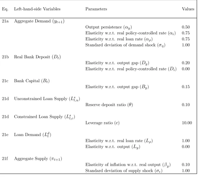
In order to simulate the model, we need to make a number of decisions, which are summarized in Table 1. First, we interpret the model as applying roughly to economic activity at an annual frequency. With this in mind, we choose our parameter values (except those parameter values related to the loan market) based on Jensen (2002). That is, the output persistence αy is
0.5; the real interest rate sensitivity of demand αi is 0.75; the sensitivity of inßation to the
output gapβy is 0.1; the weight on inßation stabilizationλis 0.8. We set the discount factor
δ to be 0.96 rather than 0.99 in Jensen (2002)5.
The difference between our benchmark (policy regime I) and alternative policy regime II mainly is a result of the fact that bank capital and deposits are both output sensitive. That is, the difference between the behaviors of output, inßation, and the optimal interest rate in the two cases depends largely on By and Dy. In an attempt to get the rough scaling
correct, we set By and Dy to be 0.15 and 0.2, respectively. The rest of the parameters are
set primarily for illustration.
5Jensen wants to use a value closed to unity so that the deviation from natural-rate hypothesis is negligible, while in our model this concern does not exist. So, we use a more conventional value.
Table 1: Calibration of the Parameters
Eq. Left-hand-side Variables Parameters Values
21a Aggregate Demand(yt+1)
Output persistence (αy) 0.50
Elasticity w.r.t. real policy-controlled rate (αi) 0.75
Elasticity w.r.t. real loan rate (αρ) 0.75
Standard deviation of demand shock (ση) 1.00
21b Real Bank Deposit(Dt)
Elasticity w.r.t. output gap (Dy) 0.20
Elasticity w.r.t. real policy-controlled rate (Di) 0.00
21c Bank Capital (Bt)
Elasticity w.r.t. output gap (By) 0.15
21d Unconstrained Loan Supply (Ls t,u)
Reserve deposit ratio (θ) 0.10 21d Constrained Loan Supply (Lst,c)
Leverage ratio (c) 10.00
21e Loan Demand (Ldt)
Elasticity w.r.t. real loan rate (Lρ) 1.00
Elasticity w.r.t. output (Ly) 0.00
21f Aggregate Supply (πt+1)
Elasticity of inßation w.r.t. real output (βy) 0.10 Standard deviation of supply shock (σ&) 1.00
They are as follows: the leverage ratio c is set to 10 (recent leverage ratio of the U.S. banking system); the reserve requirement ratio for bank deposits θ is set equal to 0.1; the output sensitivity of loan demand Ly is set to zero (for simpliÞcation); the real loan rate
sensitivity of aggregate demand αρ equals 0.756 (the conventional value for αi); the real loan
6
Our simulation tries to capture what happens when the banking system is under stress during an economic downturn. Such situation does not occur frequently. However, when it does, we believe that the coefficient before the real loan rate should become signiÞcantly larger. To avoid exaggerating the impact of credit crunch in downturns, we choose to let the value of the real loan rate sensitivity of aggregate demand be the conventional
rate sensitivity of loan demand Lρ is normalized to be unity and the real policy-controlled rate sensitivity of bank deposit Di is set to zero. Finally, the standard deviation of two
random shocks (ση and σ&) are each normalized to one. We note that we are careful to set
the parameters so that the condition needed for the Blum and Hellwig result holds.
4.2
Simulation Results
We start with a baseline experiment in which the central bank does not react to shocks at all, instead keeping the policy-controlled rate constant. To give some sense of what these pa-rameter settings mean, we compute that a one-standard-deviation purely transitory negative shock to either aggregate demand or aggregate supply drives output down by Þve times as much after four periods in the economy that is capital unconstrained.
4.2.1 Transitory supply shock
Turning to the experiment, we Þrst examine the impact of a one-standard-deviation purely transitory aggregate supply shock. That is, we set %t = 1 for t = 1, and 0 otherwise.
Furthermore, we set the initial conditions so that the economy is capital-constrained at the outset. Under regime II the central bank sets interest rates ignoring the capital constraint, using equation (24b). Under regimeI, the central bank takes account of the capital constraint and uses the interest rate rule given by equation (24a), switching to equation (24b) whenever the capital constraint no longer binds. The resulting paths for output, inßation, and the interest rate are shown in Figure 1. As we would expect, the output and inßationßuctuations are much larger under regime II when the policymakers ignore the banking system. But under regime I, since interest rates are moved aggressively in response to the negative output gap at the outset, they are less variable over the entire horizon of the simulation. The standard deviation of interest rates under regime Iand IIare 0.36 and 0.82 over 100 periods, respectively.
More speciÞcally, to offset a transitory inßationary supply shock, policy-controlled interest rate has to rise in the initial period. Over the following period, the fully-optimal policy (regime I) moves the interest rate low (aggressive) enough to counteract the procyclical effect of the binding capital constraint so that the inßation gap and the output gap are set on the optimal path.
The suboptimal policy (regime II) is conducted with the same intention as the policy regime I but fails to account for the procyclical effect of the capital constraint, therefore, doesn’t dampen the recession enough by setting the interest rate too high at period 2. InÞgure 1, from period 1 to period 9, the banking system is constrained by capital and policymakers keep conducting the suboptimal policy (regime II). However, starting from period 10, bank capital constraints are not binding under policy regime II, while the constraint always binds under policy regime I. From period 10, the inßation gap and the output gap are set on the optimal path. The suboptimal policy (regime II) generates signiÞcantly larger loss over the entire horizon. Computing the loss over a horizon of 100 periods — that is, we truncate the inÞnite-horizon objective function in equation (23) — weÞnd that the optimal policy entails a loss that is less than half the size (the simulated losses in regime Iand regimeII are 4.7 and 11.4, respectively).
4.2.2 Transitory demand shock
We examine the impact of a one-standard-deviation transitory aggregate demand shock with the same parameter conÞguration and present the paths of the output gap, inßation and the interest rate under different policy regimes in Figure 2. That is, we set ηt =−1 for t= 1, and 0 otherwise. Again, the banking system is capital-constrained at the outset.
In the period that the demand shock arrives, bank capital constraint binds. Different policy regimes cause the output gap differ in the following period. Namely, the optimal policy moves the interest rate low enough so that the output gap and inßation return to their optimal paths, while suboptimal policy fails to set the output gap and inßation on their optimal paths until period 5.
In this model, the demand shock is largely (but not completely) offset by the fully-optimal policy. Computing the loss over 100 periods, we Þnd that the simulated losses in regime I and regime II are 0.24 and 0.52, respectively. The difference between two policy regimes is signiÞcant.
As for the volatility of interest rates, the optimal interest rate is slightly variable than the suboptimal interest rate, with standard deviations being 0.25 and 0.21 over 100 periods, respectively. But the relatively high volatility of the interest rate under regime I purely comes from the strong reaction in period 1. After period 1, the interest rate is less variable under regime I.
Figure 1: Output Gap, Inßation Gap and Interest Rate with Different Monetary Policies: after a transitory supply shock.
-4 -3 -2 -1 0 1 2 1 3 5 7 9 11 13 15 17 19 21 23 25 27 29 31
outp ut_I outp ut_II
-1 -0.5 0 0.5 1 1.5 1 3 5 7 9 11 13 15 17 19 21 23 25 27 29 31 inflation_I inflation_II -5 -4 -3 -2 -1 0 1 2 3 4 1 3 5 7 9 11 13 15 17 19 21 23 25 27 29 31
interest rate_I interest rate_II
Central banks account for the impact of capital requirements in policy regimeIbut do the opposite in policy regimeII. ThisÞgure plots output gaps, inßation and interest rates for both policy regimes following a transitory supply shock given the conÞguration of parameter values in table 1.
Figure 2: Output Gap, Inßation Gap and Interest Rate with Different Monetary Policies: after a transitory demand shock.
-1.2 -1 -0.8 -0.6 -0.4 -0.2 0 0.2 0.4 1 3 5 7 9 11 13 15 17 19 21 23 25 27 29 31
outp ut_I output_II
-0.25 -0.2 -0.15 -0.1 -0.05 0 1 3 5 7 9 11 13 15 17 19 21 23 25 27 29 31 inflation_I inflation_II -3 -2.5 -2 -1.5 -1 -0.5 0 0.5 1 3 5 7 9 11 13 15 17 19 21 23 25 27 29 31
interest rate_I interest rate_II
Central banks account for the impact of capital requirements in policy regimeIbut do the opposite in policy regimeII. ThisÞgure plots output gaps, inßation and interest rates for both policy regimes following a transitory demand shock given the conÞguration of parameter values in table 1.
5
What were Central Banks Doing?
The simulation gives us some sense of how monetary policymakers should account for capital constraints. The next natural question is whether central banks in fact follow a strategy like the one our model suggests. In other words, do banks’ balance sheets and capital requirements play a material role in central banks’ decisions? In this section, we examine data to see what central banks were actually doing. To characterize the actions of central banks, we adopt the now standard framework of estimating policy reaction functions, or the Taylor rule, for the central banks of three major countries in the world: US, Germany (pre-uniÞcation) and Japan. In his original work, John Taylor (1993) characterized his now famous policy rule as a description of the Federal Reserve behavior from the mid-1980s through the early 1990s. That is, he suggested that what the FOMC actually did was to set the nominal federal funds rates so that
it=r∗+πt+ 0.5(πt−π∗) + 0.5yt, (28)
where it is the nominal federal funds rate at period t, r∗ is the natural real interest rate
(Taylor set this to 2 percent), πt is current inßation, π∗ is the inßation target (Taylor set
this to 2 percent), and yt is the percentage deviation of actual output from a measure of
potential or trend output. Clarida, Gali and Gertler (1998, 2000) have proposed estimating a forward-looking version of this interest-rate rule based on the view that policymakers are forward-looking. That is, they derive a reaction function of the form
i∗t =r∗+π∗+γπ[Etπt,k−π∗] +γyEtyt,q, (29)
where i∗t is the target rate for the nominal short-term interest rate in period t, πt,k is the
inßation from periodt to period t+k,yt,q is the output gap of period t+q,and Et(·) is the
expectation conditional on information at t. As a sufficient (but not necessary) condition for the model to be well behaved, the coefficient on inßation has to be larger than one (recall Taylor’s original rule-of-thumb was to setγπ equal to 1.5).
To see whether the central bank’s response to the output gap depends on the state of the banking system (as suggested by the theoretical models), we augment equation (29) with certain measure of the stress in the banking system. We denote the bank stress in downturns and upturns with sdt and sut,respectively. Our augmented version of equation (29) is
We let sdt−1 be thelagged deviation of the leverage ratio from its HP trend when the output gap is negative, otherwise zero;su
t−1 be thelagged deviation of the leverage ratio from its HP
trend when the output gap is positive, otherwise zero7. To address the possible endogeneity of the leverage ratio — and its response to the interest rate — we estimate the relationship with a one-quarter lag.
Based on equations (24a) and (24b), all other things equal, the policy-controlled interest rate should be lower when the leverage ratio is above-the-trend in an downturn and higher when the leverage ratio is above-the-trend in an upturn. So, if policymakers react to the stress in the banking system optimally, we expect the coefficient on sdt−1,γds, to be negative and the coefficient on sut−1,γus, to be positive.
The observed interest rate adjusts smoothly to this desired level according to the partial adjustment equation
it=Ψ(L)it−1+ [1−Ψ(1)]i∗t +υt, (31)
where Ψ(L) is a polynomial in the lag operatorL, andυtis an i.i.d. random variable that we
can think of as a monetary policy control error resulting from things like unanticipated shifts in the demand for bank reserves. Equation (31) summarizes the view that policymakers are responding smoothly to a combination of inßation and the output gap. The standard procedure is to substitute equation (30) into equation (31) and estimate the resulting equation. We estimate this model using the Generalized Method of Moments8 on quarterly data with two lags in the interest rate adjustment equation — Ψ(L) is a second-order polynomial, assuming that expectation horizon for inßation is 4 quarters. In the table below, we reported the results for two expectation horizons of output gap (0 and 4 quarters). The instrument set for the estimation includes a constant, 3 lags of short-term interest rates, inßation, output gaps, producer price inßation, M2 growth (for Germany is M3), the term spreads between the long-term bond rate and short-term interest rate, and leverage ratios.
For the U.S., our sample runs from 1989 to 2000, coinciding roughly with the Greenspan Fed era before the stock market crashed in 2000, but starting two years late to avoid the changes in the banking regulation that occurred in the 1980s. For Germany, data begin in
7
Ideally, we would like to include a measure that tracks only the banks that are under stress — what might be thought of as the marginal stress in the banking system. Our average leverage ratio is a proxy for this marginal measure since high average measure implies that there have been a relatively large number of banks with relatively high leverage ratios.
8Our estimation method relies on the assumption that all of the variables are stationary. We use the ADF test to reject the null hypothesis that there is a unit root in the interest rate or inßation for the US, Germany and Japan.
1979 and end in 1989 to avoid the impact of the uniÞcation. And for Japan, we examine the data from 1979 to 1989 to avoid the Þnancial turmoil during the 1990s in Japan.
Turning to the data, for each country we use the overnight rate that is controlled by the central bank to measure the policy interest rate; inßation is measured by the consumer price index; the output gap is deÞned as the deviation of GDP from its potential. The leverage ratio is measured as total loans of the banking system divided by the sum of bank equity and subordinated debts for the U.S., and total assets divided by bank capital plus reserves for Germany and Japan. Details of the sources and construction are described in the Appendix. Estimation also requires that we make assumptions about both the target inßation (π∗) and the target natural real interest rate (r∗). For the U.S., we assume these both to be 2 percent. For Germany, the inßation target is set at 2 percent, and the natural real interest rate is determined in the estimation. And for Japan, the inßation target is set as an HP Þltered trend, and the natural real interest rate is estimated.
Before examining the estimation results, it is useful to take a brief look at the data on the leverage ratio. The three panels of Figure 3 display data for each of the countries we study over the sample period we examine. We note that a general downward trend in both the German and Japanese data is likely related to changes in regulatory standards. For the U.S., leverage rose dramatically beginning in 1999.
Figure 3: Leverage Ratios of the United States, Germany and Japan 4 5 6 7 8 1989:02 1990:02 1991:02 1992:02 1993:02 1994:02 1995:02 1996:02 1997:02 1998:02 1999:02 2000:02 United States 25 27 29 31 33 35 1979:01 1980:01 1981:01 1982:01 1983:01 1984:01 1985:01 1986:01 1987:01 1988:01 1989:01 Germany 30 35 40 45 50 1979:01 1980:01 1981:01 1982:01 1983:01 1984:01 1985:01 1986:01 1987:01 1988:01 1989:01 Japan
Time period: US 1989q02 - 2000q04; Japan 1979q01 - 1989q04; Germany 1979q01 - 1989q04.
Data Source: US quarterly leverage ratio is the ratio of total loans (RCFD2122) and the sum of total equity capital (RCFD3210) and subordinated debt (RCFD3200), all taken from call reports. The quarterly leverage ratios of Germany and Japan are interpolated from annual data in the OECD banking data set, deÞned as the ratio of total assets and capital & reserves. The interpolation method for Germany and Japan is toÞt a local quadratic polynomial for each observation.
5.1
Estimates
Estimates of the various policymakers’ reaction functions are summarized in the three panels of Table 2. For each country we report estimates both with and without the leverage ratios (lagged and multiplied by the dummy variable that is one when output is above or below potential), and for two settings of the assumed expectation horizons for the output gap (q = 0 and 4). Thep- values of the tests of overidentifying restrictions for all speciÞcations validate the moment conditions we use. And the R2’s suggest that the models Þt relatively well.
We summarize the overall result as follows. For the US, the estimated coefficients on the inßation gap are larger than unity, implying stability, and close to the original Taylor benchmark of 1.5. The coefficients on the output gap are close or larger than the benchmark value of 0.5. Looking at the results for where the policymaker is assumed react to both current and future output gap (q = 0 and 4), we Þrst see that, while the signs of γd
s are
negative in both cases, the data donot support addingsdt−1 to the policy rule. That is, the FOMC did not react strongly to the state of banking system during economic downturns. Although the standard error forγd
s is large, it is still helpful to get some ideas of the economic
magnitude of the response. In this case, a one-standard-deviation increase in the leverage ratio equals 1.82 and that this is estimated to result in a 0.36 - percent cut in the federal funds rate, all other things equal.
Next, we see that the signs of γus are positive and signiÞcant in both cases, the data do support adding sut−1 to the reaction rule. That is, the FOMC did raise federal funds rate when the leverage ratio is high-than-trend9 during an upturn, all other things equal. The
point estimate of the coefficient is large, implying that a one-standard-deviation rise in the leverage ratio causes a 2.8-percent rise in the federal funds rate, all other things equal.
Turning to the German case, we start by noting that the coefficients before inßation and output gap are close to the original Taylor values. Turning to the banking system stress variable, to the extent that the Bundesbankdid react, it did so in a way that appears to have made matters worse. The estimate of γd
s is signiÞcantly positive and the sign of γus is both
negative and signiÞcant. These coefficients imply that a one-standard-deviation increase in leverage ratio will raise call money rate by 5 percent in a downturn and lower it by 0.9 percent in an upturn.
Our estimates for the Bank of Japan are reported in the bottom panel of the table. 9
The high leverage ratio during an upturn could be the result of credit expansion due to loan demand rather than bank capital deterioration, so we must interpret this result carefully.
For most speciÞcations, the coefficients on inßation and the output gap look a bit large. Regardless of other settings, we Þnd that the data do support addingsd
t−1 to the policy rule
but, as in the German case, the resulting coefficient estimates are of thewrong sign. To get some ideas of the economic magnitude of the response, we can compute that a one-standard-deviation rise in the leverage ratio during a downturn equals 1.56 and that this causes a 2-percent rise in the call money rate, all other things equal. As for the coefficient before
su
t−1, they are negative and insigniÞcant. Bank of Japan did not react to the stress in the
banking system in an upturn.
Taken together, the estimates of these policy reaction functions suggest that FOMC’s policy is most consistent with the model prediction, that is, to lower (raise) interest rate in response to the stress in the banking system when the economy is in a downturn (an upturn). By contrast, our results suggest that the policymakers in Germany and Japan raised their overnight interest rates, relative to the baseline, during period when output was below trend and their banks were under stress — the opposite of what our model suggests is optimal.10
6
Conclusions
Changes in bank lending are an important determinant of economic ßuctuations. Central banks, in working to meet their stabilization goals, strive to ensure a sufficient supply of loans. In their effort to maintain a stable Þnancial system, regulators can work against this objective. Capital requirements are a clear example. By dictating that all banks must maintain sufficient capital with respect to their risk exposures, capital requirements can limit the lending capacity of the banking system. Although the need for avoiding working at cross-purposes is recognized, it is not clear whether central banks have formulated an optimal strategy, namely, taken into account the impact of the capital requirements.
1 0To check the robustness, we also use alternative measures of inßation, different lags of interest rate ad-justment, the last-week policy-controlled interest rate of the quarter, the original backward-looking Taylor rule speciÞcation and different interpolation method. The robustness analysis delivers the similar overall result.
Table 2: The Reaction functions of the United States, Germany and Japan
Countries Horizon Constant Inßation Output Bank Stress Adjustment J Goodness output gap Gap Gap Downturn Upturn coefficient test of Fit
q γπ γy γds γus Ψ Adj. R2 United 0 1.28 0.61*** 0.92*** 0.87 0.95 States (0.21) (0.09) (0.01) 1.88*** 1.10*** -0.20 1.41** 0.90*** 0.87 0.95 1989q2 (0.23) (0.29) (0.33) (0.53) (0.02) - 4 1.13 0.51*** 0.94*** 0.91 0.95 2000q4 (0.30) (0.15) (0.01) 1.82** 1.31*** -0.16 1.87** 0.92*** 0.88 0.95 (0.35) (0.39) (0.48) (0.76) (0.02) Germany 0 3.62*** 1.05 -0.02 0.84*** 0.94 0.93 (0.25) (0.13) (0.29) (0.03) 1979q1 3.04*** 1.23** 0.33 6.26*** -0.67*** 0.74*** 0.98 0.94 - (0.21) (0.11) (0.21) (1.41) (0.12) (0.04) 1989q4 4 3.02*** 0.93 0.47 0.87*** 0.94 0.94 (0.55) (0.14) (0.49) (0.03) 3.00*** 1.18* 0.40 6.65*** -0.66*** 0.73*** 0.98 0.94 (0.29) (0.10) (0.26) (1.62) (0.12) (0.04) Japan 0 3.75** 1.75 1.82*** 0.83*** 0.95 0.86 (0.43) (0.67) (0.64) (0.04) 1979q1 4.22*** 1.40 1.31* 1.30*** -0.04 0.70*** 0.92 0.86 - (0.27) (0.47) (0.72) (0.37) (0.10) (0.14) 1989q4 4 3.94*** 1.75 1.19*** 0.86*** 0.94 0.86 (0.51) (0.90) (0.42) (0.05) 4.19*** 1.33 0.61 1.13** 0.09 0.75*** 0.87 0.85 (0.42) (0.65) (0.55) (0.44) (0.09) (0.14)
Estimates are by the Generalized Method of Moments, using the correction for heteroscedasticity and autocorrelation of unknown form with a lag truncation parameter of 4. The instrument set includes a constant, plus lags 1-3 of short-term interest rates, output gaps, inßation rates (CPI), changing rates of PPI and term spreads, growth rates of M2 (M3 for Germany) and leverage ratios. Robust standard errors are reported in parentheses. The sum of two adjustment coefficients (2 lags of adjustment equation for interest rate) is presented while the reported standard error is for the sum of two adjustment coefficients. The null hypothesis for the coefficient before inßation isγπ = 1. The superscripts ***, ** and * indicate that the estimations are signiÞcant at 1, 5 and 10 percent level, respectively. The numbers of observation for the US, Germany and Japan are 39, 37 and 37, respectively.
This paper does three things. First, we conÞrm the resultsÞrst derived by Blum and Hell-wig (1995) that in the presence of completely passive monetary policy, capital requirements are procyclical. That is, when banks become capital constrained shocks to the economy generate larger movements in output. Our second result is to establish that optimal monetary policy will neutralize the procyclical impact of capital requirements. That is, the capital adequacy regulation need not encumber monetary policymakers in their pursuit of their goal. Finally, we present evidence suggesting that while the Federal Reserve has been reacting as our model suggests the German and Japanese central banks clearly have not. Blum and Hellwig need not be right in theory, but they may very well be right in practice.
References
[1] Basel Committee on Banking Supervision (2001), “Overview of The New Basel Capital Accord Consultative Document.”
[2] Bernanke, Ben and Blinder, Alan S. (1988), “Credit, Money, and Aggregate Demand,” American Economic Review, 78(2) May 1988, 435-439.
[3] Blum, Jürg and Hellwig, Martin (1995), “The Macroeconomic Implications of Capital Adequacy Requirements for Banks,”European Economic Review 39 (1995), 739-749. [4] Clarida, Richard, Jordi Gali and Mark Gertler (1998), “Monetary Policy Rules in Practice:
Some International Evidence”,European Economic Review, 42 (1998), 1033-1067.
[5] Clarida, Richard, Jordi Gali and Mark Gertler (2000), “Monetary Policy Rules and Macro-economic Stability: Evidence and Some Theory,” The Quarterly Journal of Economics, February 2000, 147-180.
[6] Jensen, Henrisk (2002), “Targeting Nominal Income Growth or Inßation?" American Economic Review,September 2002, Vol. 92, No. (4), pp. 928 -956.
[7] Svensson, Lars E.O.(1997), “Inßation Forecast Targeting: Implementing and Monitoring Inßation Targets.” European Economic Review, June 1997b, 41(6), pp. 1111-46.
[8] Svensson, Lars E.O. (1999), “Inßation Targeting: Some Extensions.”Scandinavian Jour-nal of Economics, September 1999, 101(3), pp. 337-61.
[9] Taylor, John B. (1993), “Discretion versus Policy Rules in Practice,” Carnegie-Rochester Conference Series on Public Policy, December 1993, 39, pp. 195-214.
Appendix
A
Procyclical E
ff
ect of Capital Requirements in the Dynamic
Model
This appendix explains that capital requirements amplify shocks. First, according to equation (21f), we write the conditional expectation of period - t+ 1 inßation as a function of the variables known at period t
πt+1|t=πt+βyyt. (A.1)
To see the impact of bank capital regulation on real output, as aÞrst step, we put equa-tion (A.1) into the loan market condiequa-tions (equaequa-tion (21b) - equaequa-tion (21e)) to solve for the equilibrium loan rate. Substituting the equilibrium loan rate back into equation (21a), we see
yt+1 =−φji(it−πt) +φjyyt+ηt+1, (A.2)
where φji and φjy are functions of model parameters and have accounted for the impact of bank activities, and so differ depending on whetherj =cor j=u.That is,
φui = αi =φci, (A.3a) φuy = αy +αiβy− αρ LρLy+ αρ LρBy+ αρ Lρ(1−θ)Dy, (A.3b) φcy = αy +αiβy− αρ Lρ Ly+ αρ Lρ cBy. (A.3c)
Since the short-term interest rate is controlled by central banks, weÞx it at zero to see how the economy develops without an active monetary policy. With equation (A.2) and equation (21f), using a lead operator, we write real output process as a second-order difference equation (after adjusting the time subscripts) as follows:
yt= (1 +φjy)yt−1+ (φjiβy−φjy)yt−2+ςt, (A.4)
where ςt=ηt−ηt−1+αi%t−1.
than unity (assuming that neither βy or αi is zero). Two eigenvalues are λj1 = 1 +φjy+ $ (1−φjy)2+ 4α iβy 2 >1, (A.5) and λj2 = 1 +φjy− $ (1−φjy)2+ 4α iβy 2 . (A.6)
As a function of φjy and φji, eigenvalues depend on the state of capital constraint (whether
j =c orj=u).
The dynamic multiplier of the output process is eventually dominated by a function of the larger-than-unit eigenvalue λ1 as follows.
lim k→∞ ∂yt+k ∂ςt 1 (λj1)k = λj1 λj1−λj2. (A.7)
Our interest is to see the reaction of output path to a current transitory shock (%∂yt+k ∂ςt
& ) and how this changes as banks go from being unconstrained to constrained (from j = u to
j =c). In equation (A.7), %∂y
t+k ∂ςt
&
will become greater ask→ ∞since the output follows an explosive process. Equation (A.7) also tells us that the greater the values of λ
j 1
λj1−λj2 and the
larger-than-unit eigenvalue λj1 the greater the values of%∂yt+k ∂ςt
&
ask→ ∞. IfBy > 1c−−1θDy,
from computation we know that
λc1 λc1−λc2 > λu1 λu1 −λu2, (A.8) and λc1 >λu1. (A.9)
Therefore, we can conclude that %∂y
t+k ∂ςt
&
grows faster when banks are capital-constrained if
By > 1c−−θ1Dy. This is to say that the impacts of current shocks on output are ampliÞed by
B
Solution for the Dynamic Model
This appendix explains how to solve the dynamic model. The solution has four steps: (1) write down Bellman functional equations; (2) conjecture the optimal interest rate policy; (3) Þnd the value function associated with the conjectured policy; and (4) verify that the value function in step (3) satisÞes the Bellman equations in step (1).
B.1
Bellman Equations
The value functionvfor the dynamic problem should satisfy the following functional equations
v(π, y) = min i 1 2{E[λ(π+βyy+%) 2+ (1 −λ)(φuyy−αi(i−π) +η)2] +δEv(π+βyy+%,φuyy−αi(i−π) +η)} if y≥0; (B.10a) v(π, y) = min i 1 2{E[λ(π+βyy+%) 2+ (1 −λ)(φcyy−αi(i−π) +η)2] +δEv(π+βyy+%,φcyy−αi(i−π) +η)} if y <0. (B.10b)
The time subscripts are omitted since the time horizon is inÞnite. The conditiony >0(y <0) indicates that the capital constraint is not binding (binding) at the period of decision-making. The superscriptu(orc)ofφyu(orφcy)(deÞned in equation (A.2)) denotes that the coefficient is associated with the slack (or binding) constraint. Starting from the period that policymakers choosei, the output gap next period is given byφjyy−αi(i−π) +η as in equation (A.2) and
the inßation next period isπ+βyy+%.
B.2
Conjectured Interest Rate Policy and Associated Value Function
To solve the Bellman equation, instead of beginning with an initial guessv0and iterating until the process converges, it is more fruitful to conjecture the optimal policy directly, calculate the value function w associated with the conjectured policy, and then verify thatw satisÞes the functional equations (B.10a) and (B.10b).The sequence of events is as follows: Suppose period t is the period that policymakers start to solve the dynamic problem so that they can Þnd the optimal interest rate. Before the beginning of period t, πt−1 and yt−1 have been given and interest rates are set to be a
constant. At the beginning of period t, shocks %t or ηt arrive and thereby the values of πt
and yt are determined. Next, policymakers choose interest rate it before the end of period
t. Suppose the following conjectured policy is conducted in all periodst+k (k"0) starting from period t:
φuyy−αi(i−π) = b(π+βyy), ify"0, (B.11a)
φcyy−αi(i−π) = b(π+βyy), ify <0. (B.11b)
The value function w associated with the conjectured policy is calculated in two steps. The Þrst step is to add discounted loss functions λπ2
t+k+ (1−λ)yt2+k from period t+ 1 to
inÞnite with the conjectured policy implemented, conditional on the information at period t.
Note that demand shock ηt+k and supply shock %t+k are uncorrelated with each other and
across time. This step yields a function w˜(π+βyy) as follows:
˜ w(π+βyy) =δ λ+ (1−λ)b 2 1−δ(1 +bβy)2[(π+βyy)2+ δ 1−δ(σ 2 &+β2yσ2η)] +δ λσ2& + (1−λ)σ2η 1−δ , (B.12)
whereσ2η,σ2& denote the standard deviation of demand and supply shock, respectively. In the derivation, the assumption δ(1 +bβy)2 <1 is applied, which can be veriÞed after bis solved. The second step is toÞnd the value ofbby minimizing the functionw˜(π+βyy)in equation (B.12). That is,
min
b
λ+ (1−λ)b2
1−δ(1 +bβy)2 (B.13)
The Þrst-order conditon with respect tob is
λ+ (1−λ)b2 1−δ(1 +bβy)2 = − (1−λ)b δβy(1 +bβy) if λ&= 1, (B.14a) b = − 1 βy if λ= 1. (B.14b)
Note that the second-order condition also holds. The value of b is given by
b={ −(1−λ)(1−δ)−λδβ2y+ $ [(1−λ)(1−δ)+λδβ2y]2+4δ2β2yλ(1−λ) −2(1−λ)δβy , if λ&= 1, −β1y, if λ= 1. (B.15)
According to equation (B.14a), the conditionδ(1+bβy)2<1ensures that the left-hand-side is positive. On the right-hand-side of equation (B.14a), the sign of denominator depends on the sign of 1 +bβy,which is positive if inßation is persistent. It follows thatb must be negative. The value function associated with the conjectured optimal policy is obtained by replacing
b in equation (B.12) with the value in equation (B.15). That is,
w(π+βyy) ={ − (1−λ)b 2βy(1+bβy)(π+βyy) 2 −(1−λ)bδ(σ 2 $+β2yσ2η) 2(1−δ)βy(1+bβy) + δ 1−δ λσ2 $+(1−λ)σ2η 2 if λ&= 1, δ 2(π+βyy)2+12 δ2 1−δ(σ 2 & +β2yσ2η) + δσ2 $ 2(1−δ) if λ= 1. (B.16) It can be veriÞed thatw(π+βyy) satisÞes the Bellman equations (B.10a) and (B.10b).
The solution does not require to place structure on shock distributions. Consider a con-tinuous case that the density of shock η is p(η),it is in general not easy to have an analytical solution for the Bellman equation including the term Ev(η) = ' v(η)p(η)dη. However, for the capital-constraint case, the conjectured policy is linear and the associated value function is quadratic. If the shockηfollows a normal distribution, the expected value function includes the Þrst two moments of the distribution. The solution presented above works well.
In addition, it is easy to verify that the conditionδ(1 +bβy)2<1holds sincebin equation (B.15) can be rewritten as
b=− βyδl
1−λ+β2yδl. (B.17)
Equation (B.17) comes from comparing the following two equations, which hold simultane-ously λ+1−λ βy (−b) = l, (B.18a) λ+1−λ βy βyδl 1−λ+β2yδl = l, (B.18b) where lis deÞned as l= 1 2 ( λ− (1−λ)(1−δ) α2 yδ + )* λ+(1−λ)(1−δ) α2 yδ +2 +4λ(1−λ) α2 y , . (B.19)
Equation (B.18a) follows from the deÞnition ofbin equation (B.15) andl in equation (B.19). Equation (B.18b) deÞnes l.
Finally, according to equations (B.11a) and (B.11b), the optimal interest rate can be written as i = (1− 1 αi b)π+ (φ j y αi − 1 αi bβy)y, (B.20a) = Aππ+Ajyy j=u, c, (B.20b)
where band φjy are deÞned as above.
C
Data
C.1
Converting Data Frequency
When we convert high frequency data into low frequency data, we use the average observation. When interpolating low frequency to high frequency data (the leverage ratios of Germany and Japan), we Þt a local quadratic polynomial for each observation of the low frequency series, then use this polynomial toÞll in all observations of the high frequency series associated with the period. The quadratic polynomial is formed by taking sets of three adjacent points from the source series and Þtting a quadratic so that the average of the high frequency points matches to the low frequency data actually observed. For most points, one point before and one point after the period currently being interpolated are used to provide the three points. For end points, the two periods are both taken from the one side where data is available.
C.2
Data Sources
1. US short-term interest rate: quarterly average of weekly effective federal funds rate from http://research.stlouisfed.org/fred2/.
2. US consumer price index: quarterly average of monthly data from http://research.stlouisfed.org/fred2/.
3. US potential real gross domestic product: quarterly data from http://research.stlouisfed.org/fred2/.
4. US real gross domestic product: quarterly data from http://research.stlouisfed.org/fred2/. 5. Total assets of US banks: RCFD2170 in Call Reports available at
http://www.chicagofed.org/economicresearchanddata/data/bhcdatabase/index.cfm. 6. Total loans of US banks: RCFD2122 in Call Reports available at
http://www.chicagofed.org/economicresearchanddata/data/bhcdatabase/index.cfm. 7. Total equity of US banks: RCFD3210 in Call Reports available at
http://www.chicagofed.org/economicresearchanddata/data/bhcdatabase/index.cfm. 8. Subordinated debt of US banks: RCFD3200 in Call Reports available at
http://www.chicagofed.org/economicresearchanddata/data/bhcdatabase/index.cfm. 9. US money supply (M2) growth: quarterly average of annualized growth of monthly
data from http://research.stlouisfed.org/fred2/.
10. US long-term bonds interest rate: quarterly average of monthly 10-year Treasury rate from http://research.stlouisfed.org/fred2/.
11. US producer price index: quarterly average of monthly data from http://research.stlouisfed.org/fred2/.
12. Germany short-term interest rate: quarterly average of monthly call money rate from International Financial Statistics.
13. Germany consumer price index: quarterly average of monthly data from Interna-tional Financial Statistics.
14. Germany potential real gross domestic product: quarterly data from Economic Out-look 73 as published by the OECD.
15. Germany real gross domestic product: quarterly data from Deutsche Bundesbank. 16. Total assets of banks, Germany: OECD bank database. The annual data are
inter-polated into quarterly data using the conversion method discussed above.
17. Total equity of banks, Germany: OECD bank database. The annual data are in-terpolated into quarterly data using the conversion method discussed above.
18. Germany money supply (M3) growth: quarterly average of annualized growth of monthly data from International Financial Statistics.
19. Germany long-term bonds interest rate: quarterly average of monthly government bond rate from International Financial Statistics.
20. Germany producer price index: quarterly average of monthly data from International Financial Statistics.
21. Japan short-term interest rate: quarterly average of monthly call money rate from International Financial Statistics.
22. Japan consumer price index: quarterly average of monthly data from International Financial Statistics.
23. Japan potential real gross domestic product: quarterly data from Economic Outlook 73 as published by the OECD.
24. Japan real gross domestic product: quarterly data from Economic Planning Agency. 25. Total assets of banks, Japan: OECD bank database. The annual data are
interpo-lated into quarterly data using the conversion method discussed above.
26. Total equity of banks, Japan: OECD bank database. The annual data are interpo-lated into quarterly data using the conversion method discussed above.
27. Japan money supply (M2) growth: quarterly average of annualized growth of monthly data from International Financial Statistics.
28. Japan long-term bonds interest rate: quarterly average of monthly government bond rate from International Financial Statistics.
29. Japan producer price index: quarterly average of monthly data from International Financial Statistics.