c
2016
Abstract
THE MOST COMMON STREAM WIDTH IS REMARKABLY INVARIANT WITH CHANGES IN HYDROLOGIC CONDITIONS
Eric Barefoot
Under the direction of Dr. Tamlin Pavelsky
Dedication
Acknowledgements
Contents
1 Introduction 1
2 Methods 6
2.1 Study Area . . . 6
2.2 Methods . . . 7
3 Results 10 3.1 Dynamic network expansion, fragmentation, and widening . . . 10
3.2 Width distribution variation and the mode width . . . 11
3.3 Analyzing stream surface area dynamics . . . 13
4 Discussion 15 4.1 Variation of width distributions with discharge . . . 15
4.2 Spatial variation of stream width and channel geometry . . . 17
4.3 Implications for hydrology and geomorphology . . . 20
4.4 Implications for biogeochemical cycling and ecology . . . 21
4.5 Implications for stream surface area estimation . . . 22
List of Figures
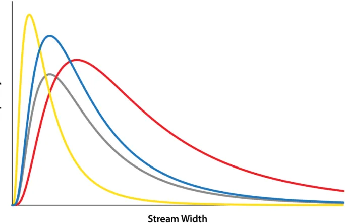
1.1 Idealized curves showing our hypotheses for dynamic stream width distributions. From an initial distribution (grey), our null hypothesis (Ho) is shown in blue, our
first alternative (H1) is shown in red, and our second alternative (H2) is shown in yellow. . . 4
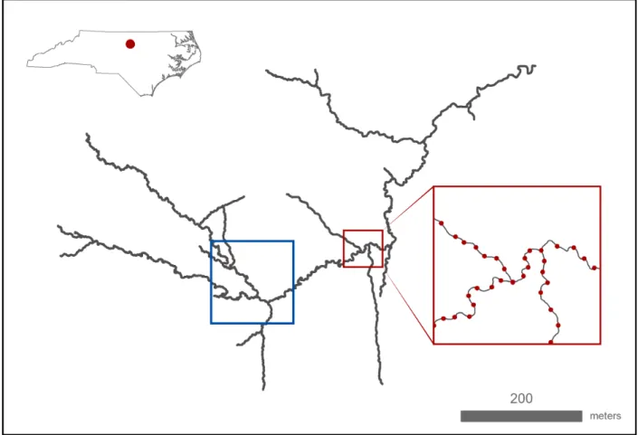
2.1 Map of study area showing location of all stream segments. The red inset shows how we constructed our sampling network, with flags spaced every five meters along the thalweg. The blue box shows the extent of the network shown in Figure 3.1. The outlet of the stream is at 79.071517◦W and 36.03909◦N. . . 7
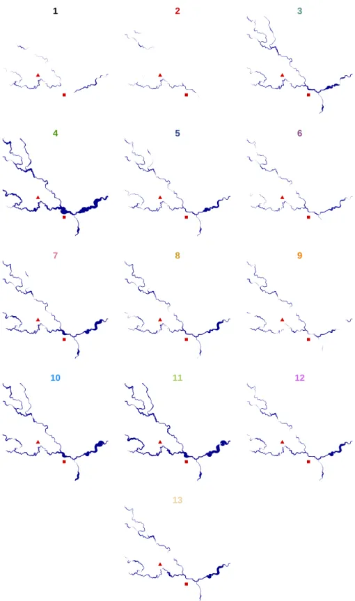
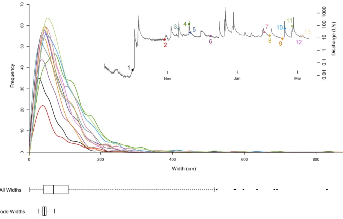
3.1 Variation in network connectivity and width across all surveys. This figure shows a subset of the basin to highlight fine-scale variations in width. The extent of this section can be seen in Figure 2.1 surrounded by a blue box. Each panel represents a unique survey, and discharge for each is shown on the hydrograph at bottom right. In order of appearance, the surveys took place during the 11th, 12th, 95th, 98th, 84th, 57th, 85th, 62th, 26th, 95th, 98th, 54th, and 56th percentiles of flow. . . 12 3.2 Using the same color scheme, we show a smoothed spline estimation of the frequency
distribution of widths during each event. Each unique event is connected to its location in the hydrograph. Additionally, we show the total variation in width as compared to the variation in modal width on the same scale as the distributions. . . 13
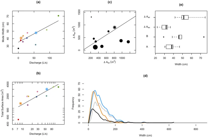
4.1 (a) Variation of mode width with discharge. (b) Power law relationship between total surface area and discharge. Connect this with Equation 3.1 (c) Selecting nine pairs of events, the increase in area due to at-a-point widening is compared to the increase due to network expansion. The relative importance of network expansion and channel widening is represented by the 1:1 line, above which expansion dominates and below which widening dominates. (d) Examining the relative balance between the two effects, distribution A shown in orange, expands to become distribution B
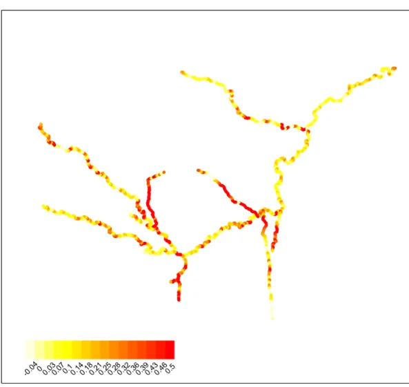
(blue) at a higher discharge and surface area. . . 16 4.2 Map of b-values calculated for Equation 1.1 using the downstream discharge for
Chapter 1
Introduction
Headwater streams are a critical natural resource. They are unique environments where different ecological, hydrologic, and biogeochemical regimes interact. Estimated to comprise nearly 66-89% of total stream length in the United States [Leopold and Maddock Jr., 1953, Allen et al., in prep., Downing et al., 2012], intermittent and ephemeral headwater streams control vital natural processes at both the watershed scale and across the entire river network [Alexander et al., 2007]. Stream width (and by extension, surface area) is an important driver of the hydrologic, biogeochemical, and ecological processes at work in these small systems.
Low order streams, typically defined as streams of order 1-3 [Alexander et al., 2007, Allen et al., in prep.], are closely coupled to groundwater. The dynamics of low order stream widths has potential to shed light on the dynamics of surface water-groundwater interactions. Stream width scales with discharge [Leopold and Maddock Jr., 1953], and therefore we expect it to be an effective measure of hydrologic conditions in headwater catchments. As such, the dynamic expansion and contraction of small ephemeral streams is a good representation of hydrologic conditions both regionally and at smaller scales [Godsey and Kirchner, 2014, Winter, 2007]. In particular, small streams reveal important characteristics of the substrate on which they flow such as hydraulic conductivity [Winter, 2007].
of changing hydrologic conditions superimposed on essentially static channel morphology. Long-term, however, water flow in the channel will alter and modify the channel geometry, feeding back onto the morphology [Rinaldo et al., 1998, Montgomery and Dietrich, 1992].
In terms of biogeochemical cycling, small headwater streams, being more tightly coupled to ground-water sources than large rivers, have a larger efflux of greenhouse gases to the environment [Allen et al., in prep., Raymond et al., 2013, Butman and Raymond, 2011]. This is largely due to the higher concentrations of CO2 in headwaters, combined with the fact that these streams are usually steeper and more turbulent than large rivers. The stream surface is an important biogeochemical interface, through which gas exchange between the hydrosphere and the atmosphere takes place. [Hynes, 1970] The speed and magnitude of that exchange is, in part, controlled by the surface area of this interface. Stream width, therefore, is an important parameter to consider when estimating CO2 efflux into the atmosphere from rivers.
In addition to gas exchange, width in small streams plays a key role in controlling water quality and solute transport to downstream reaches. Ephemeral and intermittent streams control water and solute residence times and transport across entire landscapes, modulating nutrient cycling and contaminant spread. On average, they contribute 55% of water volume and 40% of nitrogen flux into fourth and higher order streams [Alexander et al., 2007]. As such, headwaters are important potential sources and conduits for polluttion to contaminate downstream reaches. This is partic-ularly salient because in the United States, a large fraction of drinking water supplies depend on water that originates in headwater streams. In fact, nearly 58% of streams where drinking water supplies originate are intermittent streams [EPA, 2009]. Understanding the spatial and temporal variation of stream width in small headwaters catchments will help address important questions about how solutes move through these systems.
living in larger streams (e.g. salmon [Geist and Dauble, 1998]). Width and inundation area, as a measure of hydrologic connectivity and discharge throughout a catchment, can inform assessments of the suitability of a stream as a habitat, and can contribute to our understanding of the sorts of ecosystems that develop there.
Understanding the distribution of widths in small headwaters streams is critical for addressing a wide variety of questions with ecological, hydrologic, geomorphic and biogeochemical importance. The spatial distributions of width and surface area have been examined in the largest rivers [Allen and Pavelsky, 2015, Yamazaki et al., 2014] and the smallest headwater streams [Allen et al., in prep.]. At the scale of continents, river widths appear to be distributed according a power-law, and small stream widths are often characterized using similar scaling relationships. However, these simple relationships do not capture the real variability of width in time or space. Rather, recent measurement of stream widths by Allen et al. [in prep.] suggests that the frequency of widths can be modeled using log-normal distributions. Furthermore, the basic characteristics of these distributions appear to vary little across a range of mid-latitude catchments.
Despite these new findings, the variability of width and inundation extent within the smallest headwaters catchments remains poorly understood. In particular, changes in the width distribution with hydrologic conditions remain unobserved. To date, there are no consistent and complete measurements of width and surface area variability in headwater catchments. We hypothesize that changes in width distributions are driven by two factors, both increasing with discharge: lengthening of the active drainage network and widening of existing streams. Classical hydraulic geometry theory predicts that stream width will scale as a power-law function of discharge:
w=aQb (1.1)
downstream hydraulic geometry [Leopold and Maddock Jr., 1953]. This pattern implies that with increased discharge, these network expansion effects will shift the width distribution to the left,
decreasing the mode width. We predict that a balance between these factors results in relatively little change in the mode or variability of width with discharge.
Figure 1.1: Idealized curves showing our hypotheses for dynamic stream width distributions. From an initial distri-bution (grey), our null hypothesis (Ho) is shown in blue, our first alternative (H1) is shown in red, and our second
alternative (H2) is shown in yellow.
From an initial distribution of stream widthsA, we hypothesize (Ho) that with increased discharge
Chapter 2
Methods
2.1
Study Area
Figure 2.1: Map of study area showing location of all stream segments. The red inset shows how we constructed our sampling network, with flags spaced every five meters along the thalweg. The blue box shows the extent of the network shown in Figure 3.1. The outlet of the stream is at 79.071517◦W and 36.03909◦N.
2.2
Methods
To quantify patterns of stream width in response to variable discharge, we established a set of sampling locations marked by survey flags along the entire stream network at Stony Creek (740 points). This is shown in the red inset in Figure 2.1. We mapped the centerlines of the streams manually using optical imagery and GPS track data, corroborated with field observations. We placed survey flags at five meter intervals along the channel thalweg, and each flag was given a unique identifier.
a channel, including ephemeral channel features formed in leaf litter [Allen et al., in prep.]. When a stream divided into multiple channels, we visually estimated the percentage of the stream that was dry, to capture both the overall width and an index of channel braiding [Allen and Pavelsky, 2015]. When a sample location had no flowing water, a width of 0 was recorded. On occasion, new flow conditions filled channels that were previously not flagged, in which case the 5 m sampling interval was estimated by pacing. In such circumstances, we assumed that the stream segment was dry in the previous surveys. Flowing segments under five meters long, which were rare, were not mapped or recorded. Each independent event has 732 - 740 measurements, and each survey was completed in under four hours to avoid averaging over large temporal variations in discharge. Sometimes a survey flag was completely inundated, buried by sediment during large events, or washed downstream. In such cases, we recorded the width as a missing value, and later replaced the lost flag. These errors comprise a small proportion (0.00 to 0.81%) of the total number of measurements. Actual measurement error was estimated by taking the root mean squared error of paired measurements between the 12th and the 13thsurveys, which occurred within 2 hours of each other. Our root mean squared error between these surveys was 11 cm. We surveyed the stream network 13 times (n = 13) throughout the season, seeking to capture a wide range of flow conditions and seasonal variability.
For each survey, width data were paired with discharge information. Stage was measured at a 5-minute interval at the downstream-most point in the network. Discharge was then calculated from a rating curve with n = 22 points. Percentiles of flow were calculated from the long-term stage record (since September 2013). Mean discharge for each survey was then calculated from the 5-minute discharge data during the time when the survey took place. We collected surveys at a wide range of discharges spanning the 11th to 98th flow percentiles, calculated from nearly 2 years of discharge data. This range, 0.03 to 128.08 Ls, represents flows that differ by a factor of almost 4500.
Mode stream width was initially calculated from the lognormal fits. However, we preferred a different method that fits a smoothing spline interpolation (smoothing parameter 0.3) to histograms of the binned width data (bin size = 10 cm). This method produces PDFs that more convincingly match the overall shape and peak of the width distribution.
For each survey, we calculated the total stream surface area by summing the products of width and length for the whole network. We assessed the relative magnitude of at-a-point stream widening effects versus network expansion and contraction effects on stream surface area. We selected nine pairs of surveys A and B, selected so that A and B are adjacent in time and so that both the surface area and discharge of Bare greater than of A. For each pair, we calculated the total change in surface area (∆AT), then separated ∆AT into two parts. One part was the change caused by the
conversion of dry locations to wet locations (network expansion or ∆Aex) and the other was the
change in width of wet locations (at-a-point widening or ∆Awi). We then compared the relative
Chapter 3
Results
3.1
Dynamic network expansion, fragmentation, and widening
Overall, the spatial and temporal distribution of stream widths in the network is quite heteroge-neous. Stream widths across all surveys ranged from 2 to 831 cm (mean 82±61 cm), and within individual surveys the smallest range was 231, and the largest was 828. The length of active stream network varied from 800 meters to 3465 meters. Flowing widths of individual points were also highly variable. Some points varied by as much as 787 cm between surveys, while others varied little enough as to be within our root mean squared measurement error.
reach becomes quite wide. In contrast, some reaches changed very little in width despite large changes in discharge. Consider the reach marked by a triangle, which shows very little variation in width except during extreme events. Some reaches even went dry from one time to another despite an overall increase in discharge. Additionally we observed some changes in channel morphology throughout the network, for example when log-jams were cleared in large storm events, or trees fell and redirected stream flow.
In addition, our observations confirm the results of Godsey et al. [2014] that the active stream network dynamically expands and contracts in response to changing hydrologic conditions. In general, tributaries contracted from their tips before the trunk stream in the network disappeared. However this was not always the case. For example, Figure 3.1 shows the disappearance of different parts of the main trunk stream in early September, while smaller tributaries remained active. We observed significant fragmentation of the network as individual reaches within a segment went dry, as can be seen throughout Figure 3.1.
3.2
Width distribution variation and the mode width
1 2 3
4 5 6
7 8 9
10 11 12
13
Although mode stream width does not vary much compared to the overall width variation, it does vary systematically. Mode width covaries positively with discharge (b = 0.225±0.052, r2 = 0.59, p-value = 0.0012), as do the standard deviation of widths (b = 0.298±0.044, r2 = 0.79, p-value = 2.76×10⁻⁵), and mean width (b = 0.367±0.058, r2 = 0.76, p-value = 5.71×10⁻⁵).
0 10 20 30 40 50 60 70 Frequency Width (cm)
0 200 400 600 800
0.01 0.1 1 10 100 1000 Discharge (L/s) 1 2
3 4 5
6 7 8 9 10 11 12 13
Nov Jan Mar
Mode Widths All Widths
Figure 3.2: Using the same color scheme, we show a smoothed spline estimation of the frequency distribution of widths during each event. Each unique event is connected to its location in the hydrograph. Additionally, we show the total variation in width as compared to the variation in modal width on the same scale as the distributions.
3.3
Analyzing stream surface area dynamics
A=αQβ (3.1)
When comparing a pair of surveys A and B, the relative magnitudes of ∆Aex and ∆Awi are
approximately evenly distributed. In Figure 4.1 (c), points above the 1:1 line represent transitions between events where ∆Aex had a larger magnitude than ∆Awi. Further, the size of the symbol
is proportional to the surface area of event A. In general, if the surface area of event A is small, network expansion effects will be dominant, and if the surface area of event Ais large, at-a-point widening will be dominant.
Figure 4.1 (d) shows an example analysis of two such events, which are indicated in Figure 4.1 (a), (b), and (c) by circles around the relevant data points. The total change in area from the orange curve to the light blue is the total area of newly inundated reaches as added to the marginal increase in width at every point. In this case, the ∆Aex was 888.3 m2 and ∆Awi was 810.6 m2.
The width distribution from survey B can be separated into two distributions, one for ∆Aex, and
one for ∆Awi, which in Figure 4.1 (d) are plotted alongside the two distributions forA and B. In
general, the distribution for ∆Aex forms a smaller lognormal distribution close to the lower end of
the width distribution. This is represented by a dark grey line in Figure 4.1 (d). In contrast, the distribution for ∆Awi forms a very different distribution. Essentially, at-a-point widening shifts
the distribution of survey A towards higher width values and increases the spread, as in the grey curve in Figure 4.1 (d).
If the mode widths from each of these distributions (A,B, ∆Aex, and ∆Awi) is compared across
nine selected survey pairs, a pattern emerges. On the whole, the mode width of ∆Aex is slightly
narrower than mode of A, the difference is statistically significant at 95% confidence. The mode width of ∆Awi, in contrast, is significantly wider on average than the mode of A. The mode of B
Chapter 4
Discussion
4.1
Variation of width distributions with discharge
While the discharge and surface area in Stony Creek during our study varied across a large range of flow conditions, the distribution of stream widths remained comparatively stable both in location and shape. We used the mode width as our primary tool for assessing whether the distributions moved relative to each other. The mode width is much less variable compared to the total variation in width at individual points and also throughout the catchment. The total range in mode widths is smaller than the median range of at-a-point widths. In addition, the interquartile range of mode widths is almost seven times smaller than the interquartile range of all stream widths (see Figure 3.2).
We interpret the stability of the width distribution to be an indication that at-a-point widening and network expansion effects are largely in balance. This is in favor of our null hypothesis (Ho).
Indeed, in terms of added stream surface area it does not appear that there is a clear dominance of either at-a-point widening or network expansion effects. In fact, we see that for any given pair of surveysAandB, the ratio of ∆Aex to ∆Awifor each of the two effects ranges widely on either side
to high streamflow, expansion is more important, while from high to high streamflow, widening is more important (see Figure 4.1 (c)).
0 50 100
30 40 50 60 70 (a) Discharge (L/s)
Mode Width (cm)
0 10 20 30 40 50 60 70
0 200 400 600 800
(d)
Width (cm)
Frequency
200 400 600 800 1000
0
500
1000
1500
(c)
∆ Awi (m2)
∆
Aex
(
m
2)
20 30 40 50 60 70 (e)
Width (cm) A
B
5 7 10 20 30 50 80
400 600 900 2000 4000 (b) Discharge (L/s) To ta l S ur fa ce A re a ( m 2)
∆ Awi
∆ Aex
Figure 4.1: (a) Variation of mode width with discharge. (b) Power law relationship between total surface area and discharge. Connect this with Equation 3.1 (c) Selecting nine pairs of events, the increase in area due to at-a-point widening is compared to the increase due to network expansion. The relative importance of network expansion and channel widening is represented by the 1:1 line, above which expansion dominates and below which widening dominates. (d) Examining the relative balance between the two effects, distributionAshown in orange, expands to become distributionB(blue) at a higher discharge and surface area.
However, within its narrow range, mode width covaries positively with discharge and area, such as in Figure 4.1 (a). This is in favor of our first alternative hypothesis (H1), which suggests that the most common width will increase with discharge. To understand why this is, we analyzed the impacts of widening and expansion on the mode width between each pair of surveys. Despite the fact that at-a-point widening and network expansion are mostly in balance, at-a-point widening effects have a disproportionate impact on the mode width.
points that are narrower (see Figure 4.1 (d), black curve, which decreases the mode width (H2). Since the distribution of B(blue curve) is the sum of the distributions ∆Aex and ∆Awi, the mode
width of Bcan be thought of as a weighted average of the modes of ∆Aexand ∆Awi. The mode of
∆Awi is on average much larger than the mode of ∆Aex, but since the mode of ∆Aex is not much
narrower than the mode of A, widening effects pull the mode of Bto be wider than that of A. In this way, the two factors (∆Aex and ∆Awi) can be equivalent on average, but the mode width will
still increase with discharge.
We conclude that overall, surface area change in the catchment is being accommodated by both at-a-point widening and network expansion in approximately equal measure. Even so, at-a-point widening has a slightly larger impact on the distribution than does network expansion, increasing mode width and moving the width distribution slightly to the right. However, there are some practical limits to these results. In general, when discharge increased, the distribution kept the same shape and location while increasing in area. The only time when the distribution did not follow this pattern was at its highest discharge. In that survey (Figure 3.2, dark green curve), the mode width as well as the spread of the distribution increased substantially. And yet, the total area under the curve was not much larger than other surveys with high surface area. During this survey, the stream expanded to fill almost 86% of the geomorphic channel network, and was essentially only experiencing at-a-point widening effects, having very little channel to expand into. Furthermore, based on our observations in the field, this event was close to Stony Creek’s bankfull discharge. Our conceptual framework relying on channel geometry cannot explain width variation at flood stages, and therefore the implications of these findings should be restricted to discharges less than bankfull.
4.2
Spatial variation of stream width and channel geometry
simple relationships predicted by at-a-station and downstream hydraulic geometry, some reaches are usually dry, and others are often significantly wider than surrounding reaches. On average, individual measurement locations varied by 89 cm, but this variation ranged from as little as 0 cm and as much as 787 cm. The location of anomalous reaches follows no clear spatial pattern, and is not periodic.
Width does generally increase with discharge at a point as a power law (Equation 1.1). However, the variation of width with discharge throughout the catchment is unexpectedly heterogeneous. By solving for values of b across Stony Creek, we can quantify how width varies at every point in the network as a function of discharge. Lower values of b, for example, imply wide, shallow channels with steep walls [Leopold and Maddock Jr., 1953]. These b-values (mean value: 0.22±0.28) are also spatially heterogeneous. This result suggests that fine-scale stream width variability is being driven by local channel geometry. Remarkably, the mode width, and the width distribution as a whole, are quite stable despite this significant local variability in channel geometry. These results affirm the notion that the mode width is largely an emergent property of a dynamic interaction between streamflow and the geomorphic channel network.
4.3
Implications for hydrology and geomorphology
Power laws have long been used to describe hydrological systems [Leopold and Maddock Jr., 1953]. A new framework based on the collapse of fractal characteristics suggests that skewed distributions like lognormal or gamma distributions may be better descriptors than power laws of small scale hydraulic patterns. The occurrence of a similar mode width across wide ranging tectonic, climatic, and geologic settings suggests that it may be a general phenomenon with a general physical expla-nation [Allen et al., in prep.]. Furthermore, Allen et al. [in prep.] assert that using distributions with mode values implies that there may also be a most common discharge, depth, and velocity. Depth and velocity also vary at a point according to power law functions (Equations 4.1 and 4.2). A new conceptual framework based around lognormal distributions suggests that these mode values of v, d, and Q may be relatively invariant under a range of hydrologic conditions within the same watershed.
d=cQf (4.1)
v=kQm (4.2)
4.4
Implications for biogeochemical cycling and ecology
In the context of biogeochemical cycling, the heterogeneous spatial and temporal distribution of surface area should have an impact on a number of different chemical transport phenomena. For example, CO2 exsolution from streams depends on the surface area of the water-air interface. Our results demonstrate that the change in size of that interface varies widely throughout the channel network; i.e. all reaches do not increase in area at the same rate with increasing wetness. However, the width distribution remains relatively stable with increasing surface area, despite a heterogeneous distribution of surface area. Therefore we speculate that while the distribution of ∆AT is not homogeneous across the network, the local variability will not have a large impact
on the average CO2 efflux because the surface area is being added in such a way that it is not concentrated in any particular location in the network topology. The stable nature of the width distribution suggests that since widening and expansion balance each other on average, the major factor determining the total surface area will simply be total discharge (see Equation 3.1)
4.5
Implications for stream surface area estimation
This study is the first to directly measure variations in the total surface area of an entire stream system and relate it to discharge. The total surface area in a stream system can be approximated as a power function of downstream discharge measurements in Equation 3.1 (shown in Figure 4.1 (c)) (β= 0.332±0.071, r2 = 0.68, p-value = 0.0011). Because the length of the active channel network is important for the surface area, our rating curve is comparable in nature to the relationship found in Godsey and Kirchner [2014] that describes total active channel length as a function of downstream discharge. Similarly, we would expect to see highly variable β exponents across basins depending on the drainage density.
Chapter 5
Conclusions
Our results reveal spatial and temporal patterns of width in a headwater stream network. We show that stream width is spatially heterogeneous, and that the variation is a reflection of local channel morphology. Nonetheless, the stream widths in a given watershed follow a lognormal distribution, and while the total area under the curve changes with discharge, the shape and location of the distribution is comparatively stable. The peaks of these distributions, or the mode width, is an important parameter for understanding dynamics in a stream network. While the mode width varies little in comparison to the overall variability in width, it has linear relationship with discharge. As a result, we find that there is also a scaling relationship between the discharge and upstream surface area of a stream network, and that in general, surface area change in Stony Creek is driven by both at-a-point widening and network expansion. Network expansion seems to be more important at times when the network is dry, i.e. when the surface area of the network is small. The relationship between discharge and the mode width, however, suggests that the dynamic interplay between network expansion and at-a-point widening is not completely in balance.
extend this notion to hypothesize that these other mode values may be also be stable in relation to hydrologic conditions as well.
Bibliography
Richard B. Alexander, Elizabeth W. Boyer, Richard A. Smith, Gregory E. Schwarz, and Richard B. Moore. The Role of Headwater Streams in Downstream Water Quality. JAWRA Journal of the American Water Resources Association, 43(1):41– 59, February 2007. ISSN 1752-1688. doi: 10.1111/j.1752-1688.2007.00005.x. URL
http://onlinelibrary.wiley.com/doi/10.1111/j.1752-1688.2007.00005.x/abstract. George H. Allen and Tamlin M. Pavelsky. Patterns of river width and surface area revealed
by the satellite-derived North American River Width data set. Geophysical Research Let-ters, 42(2):2014GL062764, January 2015. ISSN 1944-8007. doi: 10.1002/2014GL062764. URL
http://onlinelibrary.wiley.com/doi/10.1002/2014GL062764/abstract.
George H. Allen, Tamlin M. Pavelsky, and Eric Barefoot. Uniformity of stream hydromorphology across headwater systems. in prep.
David Butman and Peter A. Raymond. Significant efflux of carbon diox-ide from streams and rivers in the United States. Nature Geoscience, 4(12): 839–842, December 2011. ISSN 1752-0894. doi: 10.1038/ngeo1294. URL
http://www.nature.com/ngeo/journal/v4/n12/abs/ngeo1294.html.
John A. Downing, Jonathan J. Cole, Carlos A. Duarte, Jack J. Middelburg, John M. Melack, Yves T. Prairie, Pirkko Kortelainen, Robert G. Striegl, William H. Mc-Dowell, and Lars J. Tranvik. Global abundance and size distribution of streams and rivers. Inland Waters, 2(4):229–236, October 2012. ISSN 2044-205X. URL
US EPA. Geographic Information Systems Analysis of the Surface Drinking Water Pro-vided by Intermittent, Ephemeral, and Headwater Streams in the U.S., 2009. URL
https://www.epa.gov/cwa-404/geographic-information-systems-analysis-surface-drinking-water-provided-intermittent. Mary C. Freeman, Catherine M. Pringle, and C. Rhett Jackson. Hydrologic
Con-nectivity and the Contribution of Stream Headwaters to Ecological Integrity at Re-gional Scales1. JAWRA Journal of the American Water Resources Association, 43(1): 5–14, February 2007. ISSN 1752-1688. doi: 10.1111/j.1752-1688.2007.00002.x. URL
http://onlinelibrary.wiley.com/doi/10.1111/j.1752-1688.2007.00002.x/abstract. David R. Geist and Dennis D. Dauble. Redd Site Selection and Spawning Habitat Use by Fall
Chi-nook Salmon: The Importance of Geomorphic Features in Large Rivers. Environmental Manage-ment, 22(5):655–669, September 1998. ISSN 0364-152X, 1432-1009. doi: 10.1007/s002679900137.
URLhttp://link.springer.com/article/10.1007/s002679900137.
S. E. Godsey and J. W. Kirchner. Dynamic, discontinuous stream networks: hydrologically driven variations in active drainage density, flowing channels and stream order. Hydrological Pro-cesses, 28(23):5791–5803, November 2014. ISSN 1099-1085. doi: 10.1002/hyp.10310. URL
http://onlinelibrary.wiley.com/doi/10.1002/hyp.10310/abstract.
Robert E. Horton. Erosional Development of Streams and Their Drainage Basins; Hydrophysical Approach to Quantitative Morphology. Geological So-ciety of America Bulletin, 56(3):275–370, March 1945. ISSN 0016-7606, 1943-2674. doi: 10.1130/0016-7606(1945)56[275:EDOSAT]2.0.CO;2. URL
http://gsabulletin.gsapubs.org/content/56/3/275.
Hugh Bernard Noel Hynes. The ecology of running waters, volume 555. Liverpool University Press Liverpool, 1970.
L.B. Leopold and Thomas Maddock Jr. The hydraulic geometry of stream chan-nels and some physiographic implications. USGS Numbered Series 252, 1953. URL
http://pubs.er.usgs.gov/publication/pp252.
Statistical Association, 46(253):68–78, 1951. ISSN 0162-1459. doi: 10.2307/2280095. URL
http://www.jstor.org/stable/2280095.
Judy L. Meyer, David L. Strayer, J. Bruce Wallace, Sue L. Eggert, Gene S. Helfman, and Norman E. Leonard. The Contribution of Headwater Streams to Biodiversity in River Networks1. JAWRA Journal of the American Water Resources Association, 43(1): 86–103, February 2007. ISSN 1752-1688. doi: 10.1111/j.1752-1688.2007.00008.x. URL
http://onlinelibrary.wiley.com/doi/10.1111/j.1752-1688.2007.00008.x/abstract. David R. Montgomery and William E. Dietrich. Channel Initiation and
the Problem of Landscape Scale. Science, 8(255):826, 1992. URL
http://www.uvm.edu/ pdodds/teaching/courses/2009-08UVM-300/docs/others/1992/montgomery1992a.pdf. Peter A. Raymond, Jens Hartmann, Ronny Lauerwald, Sebastian Sobek, Cory
McDon-ald, Mark Hoover, David Butman, Robert Striegl, Emilio Mayorga, Christoph Hum-borg, Pirkko Kortelainen, Hans Drr, Michel Meybeck, Philippe Ciais, and Peter Guth. Global carbon dioxide emissions from inland waters. Nature, 503(7476): 355–359, November 2013. ISSN 0028-0836. doi: 10.1038/nature12760. URL
http://www.nature.com/nature/journal/v503/n7476/abs/nature12760.html.
Andrea Rinaldo, Ignacio Rodriguez-Iturbe, and Riccardo Rigon. Channel Networks.Annual Review of Earth and Planetary Sciences, 26(1):289–327, 1998. doi: 10.1146/annurev.earth.26.1.289. URL
http://dx.doi.org/10.1146/annurev.earth.26.1.289.
Thomas C. Winter. The Role of Ground Water in Generating Streamflow in Headwater Areas and in Maintaining Base Flow1. JAWRA Journal of the American Water Resources Association, 43(1):15–25, February 2007. ISSN 1752-1688. doi: 10.1111/j.1752-1688.2007.00003.x. URL
http://onlinelibrary.wiley.com/doi/10.1111/j.1752-1688.2007.00003.x/abstract. Dai Yamazaki, Fiachra O’Loughlin, Mark A. Trigg, Zachary F. Miller, Tamlin M. Pavelsky, and
Paul D. Bates. Development of the Global Width Database for Large Rivers. Water Resources Research, 50(4):3467–3480, April 2014. ISSN 1944-7973. doi: 10.1002/2013WR014664. URL