EDWIN A. GOERING. Investigation of Direct Reading Passive Monitor Using Colorlmetrlc Media for Various Gases. (Under the direction of Dr. DAVID A. FRASER)
The need for an Inexpensive, direct reading, personal
monitor to measure employee exposure to workplace
atmospheric contaminants still exist. A passive monitor
using variable length orifices and the principle of
diffusion was designed and Investigated. A colorlmetrlc
media fixed at the end of the orifices was used to Indicate
contaminant relative concentration. The system was tested
with Hydrogen Chloride, Sulfur Dioxide, and Ammonia as
atmosphere contaminants. The system showed a graduated
response In relationship to the Increasing orifice lengths. Parallel scale alignment charts were prepared to allow
Interpretation of the monitor readings by the individual
employee. It is felt that the use of a system of this
nature would meet the needs of industry to provide employee
TABLE OF CONTENTS
Page
Table of Contents ... ... ... ii
Acknowledgements... iii
I. Introduction ... 1
II. Background ... ... ... 5
III. Equipment and Procedure... 13
IV. Results... 19
V. Conclusions and Recommendations ... 30
VI. References... 32
Appendices 1. Data... 35
2. Miran Calibration Charts ... 44
I wish to thank Dr. David fi. Fraser for his guidance
in this project and throughout the progress of my program.
I would also like to express my appreciation for the financial support provide by the National Institute for
Occupation Safety and Health, find to my wife and children
I. INTRODUCTION
Industrial Hygiene as an applied science frequently requires the quantitative knowledge of the level of
contaminant materials in the workplace atmosphere. The
need for determining the quantitative levels of
contaminants in the atmosphere is to insure the protection
of employees' health and safety in the workplace. Impetus for workplace contaminant level investigation may be a bona
fide interest in protecting the employees' health and
safety, an interest in protecting the financial health of
the employer from litigation by injured employee(s), or the
determination of compliance with government laws or
standards.(14)
To acquire this information, some form of air sampling is commonly undertaken. Methods commonly available today
generally utilize one of two methods.(2)
1. Personal sampling by gathering a sample of
contaminated material from as close to the breathing zone
as possible on some type of adsorption or absorption
device, into a container or other collection media for
later laboratory analysis to determine the contaminant
concentration.
monitor for the contaminant material in some predetermined
fixed location or series of fixed locations.Both of these method have drawbacks - albeit some
advantages. Method one has a significant time delay in
acquiring the quantitative data. The delay ranges from
several hours if the investigator has direct control of the
laboratory analyzing the sample to several weeks if an
outside laboratory must be contracted with to perform the
analysis. Method two, although providing instantaneous
results, is beyond the price many organizations are willing
to pay for the information. Additionally, the direct
reading instruments monitor fixed locations and may or may
not accurately reflect the actual atmosphere to which the
employee(s) is(are) exposed.
To get around these drawbacks and others of currently
available equipment, a monitoring device is needed which
will provide the required information via a direct reading
device with the following features.
1. Minimum purchase and operating cost
2. Light weight
3. Small physical size to allow convenient personal use.
4. Accurate and precise for the contaminant being
invest igated
5. Free of interference from other contaminants
6. Have a sampling range large enough to allow for
ͣ
3 7. Easily and accurately read by the user
A personal passive monitor could meet these criteria. Lippmann stated, "Personal sampling devices really began
with the development of the first lightweight portable
battery-powered pumps in about 1960. In the years since,
there have been many refinements, but if anything the samplers have become bigger and heavier rather than smaller."(8)
Uoebkenberg has reported that several manufacturers produce a variety of passive monitoring devices for a
limited number of contaminant materials.(15) Most of the
devices reported upon are not direct reading devices. That
is, they require some form of laboratory analysis following
contaminant collection. ft few of the devices are direct
reading and operate on a color change principle. Not all
these devices are truly quantitative in that they show a color change when a predetermined concentration has been
exceeded, but do not indicate to what level the
concentration exceeded the predetermined level. Mine
Safety Appliances Company is currently marketing passive,
direct reading, length-of-stain dosimeters for several
chemicals.(10,11) These devices meet most of the criteria
listed above, but still require subjective judgment as to
the actual length of the stain.
This project was undertaken to further evaluate a
passive monitor using the principle of diffusion which will
environment. It is felt that a passive monitor of this
design can overcome the drawbacks of existing equipment and
provide the required information immediately and at a
II. BPCKGROUND
The design of the monitor evaluated in this study was
based on the principle of mass transport by diffusion. Chang defined diffusion as, "The process by which
concentration gradients in a solution spontaneously decrease until a uniform, homogeneous distribution is
obtained."(3) Hinds defined diffusion as: "Mass transfer of one gas through another in the absence of fluid
flow". <6) Mass transport of contaminant gas in air to a
collecting media in a predictable way is an application of
Pick's First Law of Diffusion:(7)
J = -D (AC/AX) (eq. 1) where:
J = mass flux of the migrating contaminant (quantity of mass transported per unit
of area per unit time.)
D = diffusion coefficient of the
contaminant
Ac = negative concentration gradient that AX
exist in space, which drives or
transports the contaminant at
6
Hamm applied this equation to determine the volume of gas collected per unit area of indicator surface and
expressed it as:(5)
V/A = DC't' 60/L (eq. 3) where:
V/fi = volume of gas or vapor collected per
unit area of indicator surface at
endpoint (cm'/cm^>
D = diffusion coefficient (cm*/sec)
C = ambient concentration of gas or vapor
(ppm or cm' gas or vapor/10' cm' air)
t' = time to endpoint (min)
L = orifice length (cm)
From this equation, it can be seen that for each
orifice length a specific exposure (parts per
million-minute—ppm-min) determines spot formation for that
orifice. Accordingly, each orifice length in the monitor
corresponds to a specific exposure required for spot
formation on the collecting media, colorimetric indicator
paper, and the quantitative nature of the monitor. By
counting the number of spots that have formed, the
subjective judgment should be removed from the evaluation
of actual contaminant exposure.
The use of this mathematical derivation is based on
some assumptions which include:
7
the orifice is constant.
S. The concentration of the contaminant at the
collection media face is zero.
The achievement of these conditions in actual practice
is not always possible nor is it easily determined what is
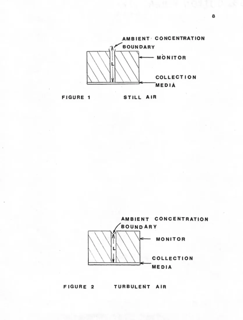
the actual condition during the period of sampling with a diffusion sampler. Figure 1 shows a diffusion tube
orifice under a static air condition. Under this
condition, molecules immediately at the face of the orifice
will start movement into the orifice and thereby lower the
concentration immediately in front of the orifice. fis time
continues, the space containing the lower concentration
increases thereby moving the point of original contaminant
concentration further away from the orifice. This
effectively increases the orifice length and thus reduces
the concentration gradient. Coulson states that an air
velocity of ten feet per minute across the face of the orifice will reduce this problem to minimal level.(3)
If the face velocity is too great, then turbulence
(convective mass transport) at the surface will cause
contaminated air to reach into the orifice and thereby
shorten the orifice length (figure 2 ). This would have
the effect of increasing the concentration gradient.
Lautenberger states that "cavities (orifices) with a length
to diameter ratio of greater than three have been used by various manufacturers to eliminate convective mass
AMBIENT CONCENTRATION
-A^BOUNDARY
i 'i> /____________
l-«--- MONITOR
COLLECTION
FIGURE 1
MEDIA
STILL AIR
AMBIENT CONCENTRATION
/^BOUNDARY
MONITOR
COLLECTION
MEDIA
9
The second assumption made in this derivation is based
on the idea that the collection surface concentration has an infinite number of active sorbent sites, thus keeping the contaminant concentration at the surface zero. In practice, the surface contains a finite number of active
sorbent sites and as these sites are filled, the
contaminant must diffuse further into the collection media
and thereby increasing the diffusion path or orifice length
(figure 3). This again would reduce the concentration
gradient. Martin states "On a theoretical basis, these errors are very small, no greater than 10%" if a diffusion sampler is operated within the design parameters of the sampler".(9)
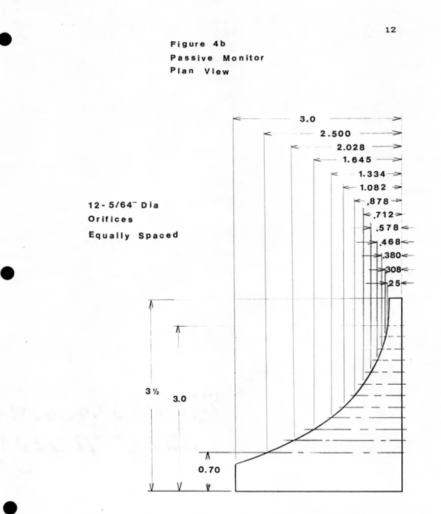
The design configuration of the monitor used in this study used logarithmically increasing orifice lengths starting with the shortest orifice length meeting
Lautenberger's criteria of length three times greater than
diameter (figure 4a and Ab). Additionally, the depth or thickness of the collection media is less than 0.007
inches. The additional orifice length due to diffusion
beyond the surface of the collection media will be well
^^VV
\1
1 ^ 1
Mon itor
Collection
Media
F i gure 3
11
FIGURE 4
PASSIVE MONITOR
CURVE In X vs. X
12 HOLES _5." DIA 64
COLORIMETRIC
Figure 4b
Passive Mo nitor Plan View
12- 5/64" Dia
Or if ices
Equally Spaced
3.0
0.70
2.500
2.028
i--- 1.64 5
1.334-^
1.082 ^
- ,8 78^
712^
.57.46
8-
•|.380-
III. EQUIPMENT fiND PROCEDURE
The concept of a passive, multiple tube, diffusion
operated monitor originated with Dr. David ft. Fraser. The
monitor evaluated in this study was a modification of the
monitor investigated by Hamm in 1981.(5) The design of the monitor in this study used exponentially increasing tube
lengths instead of linearly increasing tube lengths as
studied by Hamm.
The objectives of this project were to:
1. Prepare calibration graphs
2. Prepare Time Weighted ftverage exposure chart
for use by the monitor wearer
3. Demonstrate the feasibility of a bench model
test system.
The gases chosen for this project were Sulfur Dioxide, Hydrogen Chloride and ftmmonia. These gases were chosen because of the availability of the gas, the availability of the collection media, colorimetric paper, to detect the specific gas, and availability of proper safety equipment to handle the gases during the project. The colorimetric papers were obtained from MDft Scientific Inc. of Glenview, Illinois. MDft Scientific Inc. manufactures the paper as a
specific chemicals in industrial environments. The use of
the colorimetric paper for this project was an
extrapolation of the intent of the paper. That is, the
papers are intended to measure low concentrations of
contaminant gas, low ppm range. This is accomplished by
drawing a metered flow of contaminated air through the
paper and then reading the color change which is
proportional to the concentration of the contaminant gas
using a spectrophotometric technique.(13) In this project,
the monitor with colorimetric paper was exposed to high
concentrations of contaminant gas for sufficient duration
to allow diffusion of the gas to the paper through tubes
until spot formation occurred. The occurrence of spot
formation was determined by visual reference.
The colorimetric paper has an operating temperature
range of 0 - 40 degrees C and a relative humidity range of
10?C - 90?C. (13) The paper has a recommended shelf life of 2
1/2 to 3 1/2 months and requires refrigerated storage until
used. MDfi does not provide any information, because of its
proprietary nature, which would allow the user to test the
paper prior to use. The user has to depend on MDA's
quality control for paper reliability. Each roll of paper
is assigned a serial number. The papers used in this study
were:
Ammonia SN. 144340
Sulfur Dioxide SN. 151012
15
fill tests conducted during this study where conducted at
ambient conditions which ranged as follows:
Temperature 22.6 - 2&.0 degrees C
Pressure 747.1 - 761.0 mm HG
Relative Humidity 31 - 72%
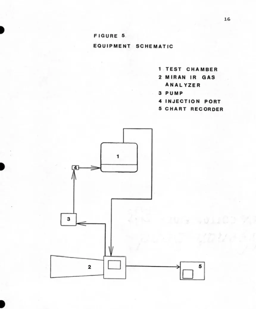
The test system consisted of an eight liter test
chamber, Miran Ifi CVF (SN lfi-3401) infrared gas analyzer. Metal Bellows Corp pump (SN16097), and interconnecting tubing in a closed loop system as shown in figure 5. fl
Cole-Palmer Linear strip chart recorder was connected to
Miran 1ft.
The Miran Ifi was used to determine the concentration
of contaminant gas in the system throughout the duration of
each trial and the chart recorder was used to record thatdata for later interpretation. fi calibration curve for
each of the contaminant gases was initially prepared using the method recommended by Foxboro Inc., manufacturer of the Miran Ifi. The data and calibration curves are shown in
fippendix 2.
Test concentrations were determined by using the
Threshold Limit Value (TLV) for each contaminant gas and calculating the ppm-minutes exposure for eight hours.(1)
That is, the TLV value in ppm multiplied by 60 minutes per
hour times eight hours. The 40S, 90?t, and 150X equivalents were then determined. Arbitrary test times were then set at 10 minutes for 40%, 20 minutes for 90%, and 30 minutes
FIGURE 5
EQUIPMENT SCHEMATIC
1 TEST CHAMBER
2 MIRAN IR GAS ANALYZER
3 PUMP
17
concentration was then calculated and the quantity of
contaminant gas needed to achieve the test chamber
concentration calculated.
Each trial was conducted by loading the monitors with the colorimetric paper and placing them on test stands in
the test chamber. The lid was placed on the chamber,
sealed and the pump started. The calculated quantity of
contaminant gas was introduced into the closed loop system through the injection port and timing was begun. The strip chart recorder recorded the Miran readings and the time of spot formation was recorded manually. Spot formation was
determined by observing a uniform color intensity
throughout an area equal to the orifice area on the side of
the colorimetric media opposite the orifice side of the
colorimetric media. ftfter all the data was collected, the
mean contaminant gas concentration for the duration of each
spot formation was calculated using the strip chart.
Trials were repeated so as to get six data points for each
spot with sulfur dioxide and ammonia and four data points
for each spot for hydrogen chloride. From this data, the
mean exposure in ppm-minutes was calculated for each spot.
To improve upon the ability to delineate spot
formation time, several steps were tried. The background
in the laboratory hood was changed from dark to light to
change the contrast. Colored lights were employed to aid
varying the room lighting was also tried. The extent of
these steps tried, did not produce noticeable improvement
IV. RESULTS
The concept of the multiple tube passive monitor
clearly is viable as seen the the photo (figure 6) of the
exposed colorimetric media. Although this is a qualitative
picture, the photo clearly shows a gradation in spot size
and color intensity from the long tube to the short tube.
The data presented in appendix 1 shows the exposure
for the experimental gases and for each spot at the three
experimental concentrations and the mean of the exposure
for each spot in parts per million - minutes. The data is
presented in graphical form in figure 7. The exposure in
ppm-minutes versus spot number is shown for each of the
concentrations tested. The plot shows a linear response as
predicted by equation 2. However, Figure 7 does show a
variability in response to concentration, but does not show
a clear relationship between changing concentration and
required exposure for spot generation. This is probably
due to the subjectivity in determining the time of actual
spot formation.
Figure fi shows the summary of the data by plotting the
mean exposure for each spot versus spot number. The lines
are nearly parallel indicating a consistent response by the
Figure 6
Figure 7
Exposuro at Tested Concentration
21
50000
20000
10000
5000
c
i
E
a
Q.
3
(0
o a X Ul
2 000
100 0
500
200
100 % of TLV
A 150% of TLV
50 » I I I I--->
I---r---r-2 3 4 5 6 7 8 9 10 11 1I---r---r-2
Figure 8
Exposure vs Spot Number
50000
20000
O -NHo
Q-HCI
V SO2
10000-5000
2000
c 1000
«" 100
1 2 3 4 5 6 7 8 9 10 ll Y2
23 Figure 9
Exposure vs Spot Number
10
c
i
E
a a.
I a>
«
o
a
ͣ
K-Ul
9
8i
6
0 NH3
ͤ
HCI
I I I
I-2345
6 7 8 9 10 11 12
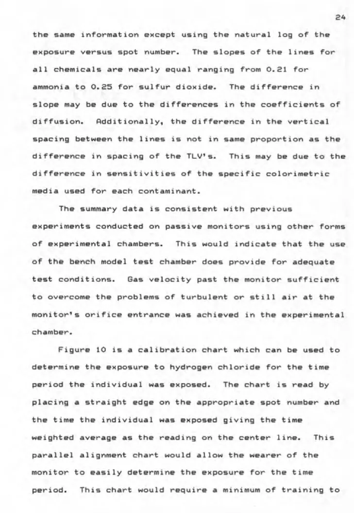
the same information except using the natural log of the
exposure versus spot number. The slopes of the lines for
all chemicals are nearly equal ranging from 0.21 for
ammonia to 0.25 for sulfur dioxide. The difference in slope may be due to the differences in the coefficients of
diffusion. Additionally, the difference in the vertical
spacing between the lines is not in same proportion as the difference in spacing of the TLVs. This may be due to the difference in sensitivities of the specific colorimetric media used for each contaminant.
The summary data is consistent with previous
experiments conducted on passive monitors using other forms
of experimental chambers. This would indicate that the use
of the bench model test chamber does provide for adequate test conditions. Gas velocity past the monitor sufficient
to overcome the problems of turbulent or still air at the
monitor's orifice entrance was achieved in the experimental
chamber.
Figure 10 is a calibration chart which can be used to determine the exposure to hydrogen chloride for the time
period the individual was exposed. The chart is read by placing a straight edge on the appropriate spot number and the time the individual was exposed giving the time
weighted average as the reading on the center line. This parallel alignment chart would allow the wearer of the
monitor to easily determine the exposure for the time
25 FIGURE 10
TIME WEIGHTED AVERAGE (TWA) EXPOSURE
HYDROGEN CHLORIDE
12i 11 10 50 9 m 8 OQ
2 7-j
I-O 6-1
allow the monitor wearer to read the results.
Additionally, this form of information presentation meets the intent of the "Right to Know" or Hazards Communications requirement for informing the employee of his/her exposure.
Additional training would be required for the specific
hazards of the particular chemicals to which the employee
is exposed to allow interpretation of the results of the
monitor reading.
Figures 11 and 12 are parallel alignment charts for
ammonia and sulfur dioxide respectively. These charts
would be used in a similar fashion to allow the wearer of
the monitor to read the time weighted average exposure for
the period of monitor use. These charts clearly show the TLV for an eight hour exposure. They could further
delineate the TLV by the use of color. For example, the section of the middle scale above the TLV could be shown in
red. This would easily allow the employee with minimal
qualifications to understand the monitors reading.
Additionally, the middle scale could be colored yellow in
the action level range and green below the action level.
Different styles of charts were reviewed for use as a
method to easily allow the monitor wearer to determine
exposure. Trilinear charts were considered, but were
determined to be too confusing for quick and easy
interpretation. Leaving the chart in the form of figure 8
was considered, but this chart would require division of
27 FIGURE 11
TIME WEIGHTED AVERAGE (TWA) EXPOSURE
AMMONIA 12t 11 10 9 CD
Z 7
O 6
FIGURE 12
TIME WEIGHTED AVERAGE (TWA) EXPOSURE
SULFUR DIOXIDE
UJ 12 11 10 g 8 00 s
2 7
29
(TWO) concentration and would lead to many errors.
Therefore, the parallel scale alignment chart was chosen as
the best form of information presentation considering that
it would be used by relatively untrained employees.
Other types of devices such as circular slide rule type
V. CONCLUSIONS ftND RECOMMENDATIONS
The monitor as tested demonstrated consistent results over the three chemicals. The linearity of the response
shows that the monitor performs as predicted. With
calibration charts prepared for a given chemical and these charts converted to easily interpreted TWft diagrams the monitor can be used to give satisfactory results for use by
the typical employee.
However, for the monitor to gain a wide acceptance in the field of Industrial Hygiene, several improvements
should be made to the system:
1. The colorimetric media must be designed specifically for this application with the idea in mind that the monitor will be read by the human eye under
varying conditions of light.
2. The change in color due to contaminant reaching
the collection media should be made more pronounced.
3. ft wider range of collection medias must be
developed for the more commonly used chemicals in the
workplace.
It is clear to this researcher that the diffusion operated, passive monitor has good commercial potential.
31
material and small in size. The use of injection molded or
even thermoformed plastic monitors would make the monitor a low initial cost item. Each device would probably be low
enough cost that each monitor would be a one time use
device. The one time use cost would have to be balanced against the cost of labor and handling to refill a multiple use monitor before each use with the collection media. The
cost of the collection media for this experiment was $36.25
(retail) for 240 strips. These cost factors along with the
ease of use and rapidity of results should make the system
acceptable in the market place.
Further research is needed to determine the TWO charts
for other commonly used chemicals and the appropriateness
of the passive monitor device for these chemicals.
To further test the monitor, it should by used
experimentally in a lifelike situation with movement
through the contaminated environment similar to movement by
a working employee.
ft modification of the monitor which might provide for easier determination of which spot to consider the endpoint would be to create a monitor with fewer holes spaced
1. American Conference of Governmental Industrial
Hygienists, Threshold Limit Values for Chemical Substances in the Uiork Environment Adopted by flCGIH for 1964-85.
fiCGIH, Cincinnate, OH, 1984.
2. Brief, R. S., "Sampling for Gases & Vapors", Basic Industrial Hygiene fl Training Manual. Winter 1975
Supplement to the Medical Bulletin, Exxon, New York, 1975, pp. 47-55.
3. Chang, R., "The Liquid State", Physical Chemistry with Applications to the Biological System, 2nd ed., Macmillan,
NY, 1981, p83.
4. Coulson, D. M., "Method Validation", AnnaIs of
American Conference of Governmental Industrial Hyqienists.
Vol. 1, pp. 83-89, 1981.
5. Hamm, M. E., Design and Evaluation of A Direct-Reading Passive Monitor for Gases and Vapors, Master's Technical Report, Department of Environmental Sciences and Engineering, School of Public Health, University of North
Carolina at Chapel Hill, 1981
6. Hinds, W. C., "Properties of Gases", Aerosol Technology - Properties. Behavior. & Measurements of
Airborne Particles. 1 ed., Wiley, New York, 1982, p. 23.
7. Lautenberger, W. J., Kring, E. V., and Morello, J. A.,
"Theory of Passive Monitors", Annals of American Conference of Governmental Industrial Hygienists. Vol. 1, pp.91-99,
1981.
8. Lippmann, M., "Dosimetry for Chemical Agents: An Overview", Annals of American Conference of Governmental
Industrial Hygienists. Vol. 1, pp. 11-21, 1981.
9. Martin, J. E., "An Intuitive Approach to Passive Monitors", Annals of American Conference of Governmental
33 10. McConnaughey, R. W. , McKee, E. S. , Pritts, I. M. ,
"Passive Colorimetric Dosimeter Tubes For Pmmonia, Carbon
Monoxide, Carbon Dioxide, Hydrogen Sulfide, Nitrogen
Dioxide and Sulfur Dioxide", ftitierican Industrial Hygiene
Association Journal, Vol. 46, No. 7, pp. 353-362, July
1985.
11. McKee, E. S., McConnaughey, P. W., "Passive, Direct
Reading, Length-of-Stain Dosimeter for Ammonia", American
Industrial Hygiene Association Journal. Vol. A5, No. 8, pp.
407-AlO, Aug, 1985.
12. McMahon, R., Personal Communications, Oct. 10, 1965.
13. MDA Scientific, Inc., "Series 7100 Continuous Toxic
Gas Monitor", Data Sheet No. 970372, Jun 1985.
14. Occupational Safety and Health Administration, General
Industry Safety and Health Standards (29 CFR 1910), U. S.
Department of Labor, Washington, D. C., 1976, p 504-510.
15. Woebkenberg, M. L., "Personal Passive Monitors for
Chemical Agents", Annals of American Conference of
Goyernmental Industrial Hyqienists, Vol. 1, pp. 107-115,
35
Ammonia
Exposure for spot formation (ppm-mlnute)
Spot # Percent of TLV Concentration
Spot
Trial # 40*/. 90*/. 150*/. Mean
1 la 3539 3296 321S
lb 3494 3296 3216 2a 3613 2224 3581 2b 3654 2224 3267 3a 2961 2668 3475
3b 2961 2792 3678
3175
ean 3370 2750 3405
la 4615 4060 4750
lb 4696 4060 4768
2a 4375 3581 4187
2b 4389 3581 4187
3a 3847 3602 4080
3b 3847 3692 4118
Mean 4295 3763 4348 4135
la 6466 5212 5225
lb 5852 5212 5225
2a 5576 4749 4862
2b 5643 4565 4862
3a 4615 4677 4742
3b 4615 4959 4999
Mean 5461 4896 4986 5114
la 8559 6530 7248
lb 8386 6472 7248
2a 8742 5431 6242
2b 8368 5258 6496
3a 5723 6428 6613
3b 5723 6428 6656
la 10697 6223 9810
lb 10415 6060 9810
2a 10655 7227 7425
2b 10655 6843 7216
3a 7366 6036 8916
3b 7060 8145 9386
Mean 9475 7756 8310 8514
la 13145 10310 11931
lb 13278 10263 11931
2a 11693 9578 9977
2b 11424 8621 9064
3a 9636 9810 11178
3b 8970 9810 11241
Mean 11356 9632 10887 10659
la 17303 15847 13758
lb 17820 13417 13758
2a 12843 12797 12933
2b 13656 11016 12001
3a 12388 12378 13511
3b 11573 12378 13549
Mean 14264 12972 13252 13496
a la 19855 19045 16942
lb 20002 19099 16890
2a 17417 15384 16693
2b 17826 14761 15399
3a 14342 16174 15686
3b 13195 16174 17182
Mean 17106 16773 16465 16781
la 26104 22557 19748
lb 26344 19911 19748
2a 23379 18052 20977
2b 23379 17434 18357
3a 17896 18864 17567
3b 17009 18969 20769
37
lO la 31810 24933 26349
lb 30937 21874 26349
2a * 20281 26099
2b «ͣ 20253 24228
3a 21063 24602 21828
3b 21063 25833 27270
Mean 26218 22963 25354 24673
11 la 37809 28213 30621
lb 38648 25485 34732
2a « 23744 28684
2b » 23583 28511
3a 22904 27958 28978
3b 22904 28958 27748
Mean 30566 26323 29879 28717
12 la * 34816
lb * 33076 *
2a 29190 36290
2b 28518 37059
3a 26676 31840 36713
3b 26676 33741 37260
Hydrogen Chloride
Exposure for spot formation <ppm-minute)
Spot # Percei
Spot
Trial # 40%
1 la 360.4
lb 360.4
2a 412.5 2b 412.5
Percent of TLV Concentration
Mean 386.5 90% 657.0 680. 5 347.8 361.0 511.6 150*/. 357.0 357.0 625.0 625.0 491.0 Mean 463.0
la 456.5 820.1 431.4
lb 456.5 834. 1 431.4
2a 600.4 468.0 699.2
2b 600.4 532.7 699.2
Mean 528.5 663.7 565.3 585.8
la 589.3 1022.1 497.2
lb 589.3 1096.3 497.2
2a 856.3 839.0 1090.3
2b 856.3 931.9 1090.3
Mean 722.8 972.3 793.7 829.6
la 798. 5 1196.9 808.5
lb 798. 5 1386.8 1000.7 2a 983. 1 1231.6 1181.1 2b 983. 1 1231.6 1181.1
ean 890. 8 1261.7 1042.8 1065.1
la 1001. 9 2152.7 1358.0 lb 1001. 9 1663.2 1459.9 2a 1117. 6 1605.1 1285.9 2b 1117. 6 1605.1 1699.9
39 la lb 2a 2b Mean 1346.9 1346.9 1245.3 1245.3 1296.1 2330.6 2152.7 2131.2 1879.8 2123.6 1907.3 2315.9 2089.8 2041.6 2088.6 1836.1 la lb 2a 2b Mean 1725.0 1725.0 1493. 5 1493.5 1609.2 2906.1 2804.0 2633.4 2442.8 2696.6 2676.7 2928.2 2392.9 2705. 8 2675.9 2327.2 a la lb 2a 2b He m 2363.8 2363.a 1972.7 1972.7 2168.2 3158.1 3009.6 3521.5 2861.7 3137.7 3389.6 3576.0 3248.7 3080.4 3323.7 2876.6 la lb 2a 2b He tn 2830.7 2830.7 3019.1 2457.1 2784.4 3766.0 3366.5 4294.7 3594.5 3755.5 4570.3 4324.6 4056.a 4268.9
4305. 2 3615.0
10 la lb 2a 2b Hean 3436.4 3436.4 4130.8 4410.0 3853.4 4519.8 4565.5 5670.3 5362.7 5029.6 5383. 5 5820.1 4676.3 5085. 6 5241.4 4708.1 11 la lb 2a 2b Hean 3699.5 3699.5 5189.1 5189.1 4444.3 5474.2 5951.1 6348.4 5757.2 5882.a 7007.2 7711.0 5293.4 6707.0 6679.7 5668.9 12 la lb 2a 2b 4195.3 4195.3 5730.8 5730.8 6758.9 7724.2 6869.5 6891.9 8888.9 9662.0 5931.4 9400.1
Oi tJ -H a 0 ͣ H a u 3 «H H 3 cn 01 -fj 3 C •H E I E a a c 0 •H +> (0 e u 0 «H +• 0 a ID u 0 «H 01 u 3 Q) 0 a u a Qi s C 8 0 in
-H H (0 c 01 0 c 0 U X > J H <H 0 +» c 01 u u 01 0. 8 01 8
8 in '* ^ in n
oi 8 in in n "H S CO 8 8 "H 8
01 8
® f, h> Q CO •H
• ͣ••••
CO «J3 iJ) 8 iJ3 ts 01 8 n '^ 00 00
^ H ^ H H
in
U) [^ U} iD 8 8
8 (N 8 CN ci C) 8 8 ^ (N CM CM
^ ^ H H ^ ^
H n in CO (N CN
• •••••
01 (N in 8 00 CO d n 00 01 n n
n
VD N CO 8 01 "H -H 00 8 CN '* ^ in in h- 00 cn n -H ^ CN CN CN CN
01 (D u3 r^ in 0) 8 (N in (N CN CN
-H CO -H '*' (N CN ^ CO 01
01 01 '*
^88 in u) u) H »H n cn n n
8 00 CN 00 CN 8 cn
C^l in cn in CO cn ^ CN in ^> IS cn cn CO 8 8
ͣH -< -^ CN CN ^ CN CN
n 01 uQ t^ on ^
• •••••
00 lO t^ cn f^ CO fs 0) cn cn ^ CO N CN CN CN CN (N
00
CO in H CO uj cn
uD oi CN 8 in ^
CP 01 »H "H "H 8 0»
8
CN UD 8 8 00 CS
• •«•••
in 8 00 CO ^ cn CN cn in in in in
^ ^ ^ ^ ^ ^
UD cn CN ^ h. 00 01
« ••••••
N UD 8 kO 8 CO C4
ͣ
f U) 01 CO 00 CN CN ^ ^ ^ H »H ^^l CN
00 in 01
CN CO CO t^ tN t*.
• •••••
8 00 in n 0) h> in 01 in CN in 0) (N CN (N CN CN CN
00 in CN
c c
H (0 .Q (0 X] <0 Jl (0 (D J3 (0 ^ CD .Q a a H -H (N CN cn cn 01 ^ H CN CN cn OJ 01
-H £ s
(h H
(0 XI
c c
at X] (D J3 0 (0 XI (0 XI (0 XI (0 CN CM cn cn 01 »H -H CN CN cn cn 01
41
8
la 325.7 407.2 273.5
lb 330.4 389.8 269.0
2a 303. 1 434.4 449.4
2b 260.6 438.1 456.5
3a 332.2 336.1 414.2
3b 337.4 411.9 413.3
Mean 314.9 402.9 379.3 365.7
la 402.5 547.6 358.9
lb 394.1 555.0 378.4
2a 424.5 532.8 556.4
2b 371.4 532.8 572.5
3a 458.2 540.9 570.2
3b 465.6 552.6 575.5
Mean 419.4 543.6 502.0 488.3
la 446.1 658.5 518.7
lb 476.4 640.9 521.4
2a 501.5 630.0 706.2
2b 552.2 630.0 690.4
3a 599.5 643.7 686.9
3b 605.3 749.8 653.8
Mean 530.2 658.1 629.6 606.2
la 525. 2 810.8 748.7
lb 530.6 700.7 755.7
2a 604. 1 743.4 988.0
2b 640.9 743.4 988.0
3a 809. 6 807.4 870.5
3b 866.2 837. 1 873.2
Mean 662.8 773.8 870.7 769.1
la 712.0 844.0 945.1
lb » * *
2a 748.6 895.0 1150.3
2b » » *
3a 1057.9 1055.4 1159.1
3b • *
10 11 12 la lb 2a 2b 3a 3b 937. 9 1075.4 920.7 1227.8 1347.1 1413.2 1166.9 920. 1 1065.3 1095.4 1233.8 1444.9 1206.1 1212.2 1297.9 1320.6 1386.0 1398.0
ean 1153. 9 1154. 4 1303. 5 1203.8
la 1314. 0 1316. 7 1468.4 lb 1375. 2 1135. 7 1460.2
2a 1415. 8 1254.7 1441.2 2b 1570.2 1250. 3 1443.6
3a 1639. 5 1491. 8 1474.9 3b 1656. 9 1581. 7 1477.4
ean 1495. 3 1338. 5 1460.9 1431.6
la 1592. 0 1927. 1 1648.5
lb 1598. 5 1820. 9 1653.2
2a 1727. 2 1904. 0 1756.9
2b 1863. 7 2035. 7 1793.9 3a 1992.2 1765. 2 1621.2
3b 2000. 0 2159. 7 1783.6
APPENDIX 2
•)
220
WIRAN 1A CALIBRATION CHART for HCL
K- 140
0.070 0.080 0.090 0.100 0.110 0.120 0.130 0.140
ABSORBANCE
551
MIRAN 1A CALIBRATION CHART for S O2
0,04 0.08 0.12
0-16 0.20 0.24 0.28 0.32 0.36 0.40 0.44
ABSORBANCE
800
700
E
a
Q. 600
z
O
H
< 500
1-Z UJ
O z
o
o 400
300 0.22
MIRAN 1A CALIBRATION CHART for NH3
0.24 0.26 0.28 0.30 0.32 0.34
47
Miran lA Calibration Chart for HCl
Ambient Conditions
Temperature: 23.3 C
Barometric pressure: 747. 1 mm Hg Relative Humidity•
• 50'/.
Equipment Settings
Wavelength: 3.40 um
Pathlength: 20.25 m
Slit width: 1 mm
Gain: XI
Meter Response: 1
Injected System Absorbance
Volume Cone. Trial Trial Trial Trial
ul ppm # 1 # 2 # 3 # 4 Mean
400 70.9 0.069 0.072 0.074 0.075 0.072 480 85.1 0.069 0.077 0.082 0.077 0.076 560 99.3 0.075 0.085 0.086 0.084 0.083 640 113.5 0.082 0.091 0.092 0.090 0.089 720 127.6 0.089 0.098 0.098 0.096 0.095 800 141.8 0.095 0. 103 0. 104 0.101 0.101 880 156.0 0.100 0.109 0.109 0.107 0.106 960 170.2 0. 105 0. 115 0.115 0.112 0. 112 1040 184.4 0.111 0. 120 0. 121 0. 117 0. 117
1120 198.6 0.116 0. 125 0. 125 0.122 0. 122
Miran lA Calibration Chart for S02
Ambient Conditions
Temperature: 23 C
Barometric pressure: 757. 6 mm Hg
Relative Humidity: 31'/.
Equipment Settings
Wavelength: 7.42 um
Pathlength: 20. 25 m
Slit width: 1 mm
Gain: XI
Meter Response: 1
Injected
Volume ul
System
Cone, ppm
Absorbance Trial Trial
#1 #2
Trial
# 3 Mean
30 5.3 0. 049 0.051 0.055 0.052
60 10.6 0. 099 0.100 0. 104 0. 101
90 16.0 0. 145 0. 146 0. 144 0.145
120 21.3 0. 192 0.189 0. 186 0.189
150 26.6 0. 237 0.230 0.232 0.233
180 31.9 0. 270 0.270 0.272 0.271
210 37.2 0. 312 0.312 0.318 0.314
240 42.6 0. 353 0.351 0.360 0.355
270 47.9 0. 395 0.389 0.399 0.394
49
Miran lA Calibration Chart for NH3
Ambient Conditions
Temperature: 26 C
Barometric pressure: 752.4 mm Hg
Relative Humidity•
• 66X
Equipment Settings
Wavelength; 10.5 jm
Pathlength: 20.25 m
Slit width: 1 mm
Gain: XI
Meter Response: 1
Injected System Absorbance
Volume Cone. Trial Trial Trial Trial
ul ppm # 1 # 2 # 3 # 4 Mean
1800 319 0.241 0.200 0.209 0.248 0.224
2000 355 0.241 0.218 0.211 0.250 0.230
2200 390 0.249 0.229 0.223 0.260 0.240 2400 426 0.258 0.240 0.237 0.270 0.251 2600 461 0.264 0.251 0.249 0.280 0.261 2800 496 0.272 0.257 0.260 0.290 0.270
3000 532 0.281 0.265 0.270 0.300 0.279 3200 567 0.291 0.274 0.280 0.309 0.289
3400 603 0.300 0.286 0.289 0.318 0.298 3600 638 0.308 0.293 0. 298 0.326 0. 306
51
Physical Properties
Ammonia Hydrogen Sulfur
Chloride Dioxide
Formula NH, HCl SOe
Formula 17.03 36.47 64.06
weight
Diffusion <12) 0.2204 0.1684 0.1386 coefficient
cm'/sec
Solubility 89.9 82.3 22.8
grams in water 0° C