Vol. 12, No. 2, pp 253-269
On Exponential Power Distribution And Poultry
Feeds Data: A Case Study
A. A. Olosunde
Department of Mathematics, Obafemi Awolowo University, Ile-Ife.
Abstract. In this paper, we propose to study a generalized form of the exponential power distribution which contains others in the literature as special cases. This unifying exponential power distribution is charac-terized by a parameter ω and a function h(ω) which regulates the tail behavior of the distribution, thus making it more flexible and suitable for modeling than the usual normal distribution, while retaining sym-metry. We derive several mathematical and statistical properties of this distribution and estimate the parameters using both the moments and maximum likelihood approach, obtaining the information matrix in the process. The multivariate extension of the distribution is also examined. Finally we fit the univariate generalized exponential power distribution as well as the normal distribution to data on eggs produced by chicken on each of two different poultry feeds (inorganic and organic copper-salt compositions) and show that the generalized exponential power distri-bution fit is considerably better. We then use the Kolmogorov-Smirnov two samples one-tailed test to show that there is an increase in egg weights and decrease in cholesterol level when the feed is organic. Keywords. Exponential power distribution, information matrix, inor-ganic copper-salt, maximum likelihood estimation, multivariate expo-nential power distribution, organic copper-salt, poultry feeds data. MSC: 60E05, 62H10, 6207.
Olosunde( )([email protected]) Received: June 2012; Accepted: November 2012
1
Introduction
The exponential power distribution is a class of densities which includes the normal and allows thick tails, Thus making it more suitable in mod-eling when compared with the usual normal distribution. In fact, it is a natural generalization of the normal distribution and first introduced by Subbottin (1923). Gomez et al. (1998) presented a multivariate version of the exponential power distribution and Lindsey (1999) used this dis-tribution to model repeated measurements. We begin this section with a proposition.
Proposition 1.1. let X be a random variable then,
f(x;µ, σ, ω) = ωh(ω) 2Γ(1ω)σexp
{
−
[
h(ω)|x−µ| σ
]ω}
is a probability density function (p.d.f.) with three parametersω >0,
σ > 0, µ∈ ℜ. The tail region is regulated by the function h(ω), which is positive for all ω >0.
Proof. Since
f(x;µ, σ, ω) = ∫ ∞
−∞
ωh(ω) 2Γ(ω1)σ exp
{
−
[
h(ω)|x−µ| σ
]ω}
dx= 1, (1)
where µ ∈ IR and σ ∈ (0,∞) are respectively, location and scale pa-rameters and the function h(.) for all ω > 1 is positive, the theorem is proved
Note that (1) reduce to: (i) Subbottin (1923) distribution if h(ω) = 1
ω; and (ii) Univariate power exponential distribution studied by Gomez,
et. al. (1998), whenω = 2β and 2h(ω) = 1. The functionh(ω) regulates the tail region, hence the distribution is more flexible when compare to normal distribution.
Remark 1.1. We note that the density in equation (1), henceforth called a generalized form of the exponential power density (GEP), was developed from the data (see Appendix B) obtained in the experiment carried out on poultry feeds data. The model gave a better fit when compared with the normal distribution.
By symmetry, the odd central moments are zero. If the random variable
X follows a GEP distribution we may writeZ = (Xσ−µ). Then the nth moment of Z is
E(Zn) = 1 + (−1)
n
2Γ(ω1) h(ω)
1−n+1ω Γ(n+ 1
ω ). (2)
Hence the kth moment ofX is
E(Xk) =E[(µ+σZ)k] Now, using binomial expansion we have;
n ∑ k=0 ( n k )
µn−kσkE(Zk) = Σnk=0µn−kσk1 + (−1)
k
2Γ(ω1) (h(ω))
1−nΓ(k+ 1
ω )
Proposition 1.2. The following expressions for the mean, variance, and Kurtosis of a random variableX ∼GEP(µ, σ, ω) hold:
E(X) =µ;
E(X2) = h(1ω) {
µ2+σ2Γ(
3
ω)
Γ(ω1)
} ;
E(X3) = [h(ω1)]2
{
µ3+ 3µσ
2Γ(3
ω)
Γ(ω1)
}
and
E(X4) = [h(ω1)]3
{
µ4+ 6µ
2σ2Γ(3
ω)
Γ(ω1) + σ4Γ(5
ω)
Γ(ω1)
}
Proof. The proof follows easily from the above expressions for the binomial expansion. The skewness is obviously zero as for the case of normal distribution.
2
Maximum Likelihood Estimation
Given a random sample ofn observationsx1, ..., xnfrom the generalized
exponential power distribution, then the log-likelihood function ℓis:
ℓ(θb) =nlnω+nlnh(ω)−nln 2−nln Γ(1
ω)−nlnσ−
n
∑
i=1
[
h(ω)|xi−µ|
σ
]ω
The likelihood equations for the three parameters are obtained by dif-ferentiating with respect toµ,σandωrespectively and equating to zero. We have:
∂ℓ ∂µ =−ω
[
h(ω)
σ
]ω∑n i=1
|xi−µ|ω−1sgn(xi−µ) = 0 (3)
where
sgn(xi−µ) ≡
1, if xi > µ
0, if xi =µ −1, if xi< µ
∂ℓ ∂σ =
−n σ +ω
−ω−1 n
∑
i=1
[
h(ω)|xi−µ|
σ
]ω
ˆ
σ = h(ω) ( ω n n ∑ i=1
|xi−µ|ω
)1 ω , (4) and hence ∂ℓ ∂ω = n ω +
nh′(ω)
h(ω) −
nΓ′(1/ω) Γ(1/p)
−
{[
h(ω)
σ
]ω
ln
[
h(ω)
σ
]
+ p[h(ω)]
ω−1
σω
} n ∑
i=1
|xi−µ|ω −
[
h(ω)
σ
]ω∑n i=1
|xi−µ|ωwi(µ) = 0 (5)
where
wi(µ)≡
{
ln|xi−µ|, if xi ̸=µ
0, if otherwise
The prime (′) denote the differentiation with respect to ω. The joint likelihood equations for µ, σ and ω can be solved by simultaneously solving equations 3-5. The Fisher information matrix I(µ, σ, ω) when n=1,has elements−E[∂2lnf(x, θ)/∂θi∂θj
]
fori, j= 1,2,3,, whereθare the parameters under consideration in GEP distribution. The variance-covariance matrixI−1(θ) of the ML estimates µ, σ, ω.
E
(
−∂2lnℓ
∂µ2
)
= ω(ω−1)[h(ω)]
2Γ(1− 1 ω)
σ2Γ(1 ω)
(6)
E
(
−∂2lnℓ
∂µ∂σ
)
= 0 (7)
E
(
−∂2lnℓ
∂µ∂ω
)
= 0 (8)
E
(
−∂2lnℓ
∂σ2
)
= ω−n+ 1
σ2 (9)
E
(
−∂2lnℓ
∂σ∂ω
)
= − 1
σω
[ 1 +ω
2h′(ω)
h(ω) +ψ(1 + 1
ω) +ωlnh(ω)
] (10) and
E
(
−∂2lnℓ
∂ω2
)
= n
ω2 −
nh(ω)h′′(ω)−[h′(ω)]2 [h(ω)]2
− nΓ(ω1)ψ
′
(ω1)−[ψ(ω1)]2 [Γ(ω1)]2
+ ω
[
h′(ω)
h(ω) ]2
−h′(ω) + [
h′(ω)
h(ω) ]2
− h
′
(ω)
h(ω) [
ψ(1 + ω1)
ω + lnh(ω)
]
− h ′′
(ω)
h(ω) −
h′(ω)
ωh(ω) (11) from this matrix obviously the shape parameterω is orthogonal to the location parameter µ, but is not orthogonal to the scale parameter,σ.
3
The Multivariate Extension
Several authors (e.g. Gomez et al., 1998 and Fang et al. 1990) have studied the multivariate extension to the usual exponential power dis-tribution. The procedure in Fang, et al. (1990) may be applied to the standard univariate density function,f(x2) defined for (1) as;
f(x2) = dF(x;ω)
dx = ωh(ω) 2Γ(ω1)exp
{
−[h(ω)x2]ω2
}
(12) replacingx2 in (12) by the Mahanalobis (1936) distance ∆2Σ(x, µ), gives
dF(x;µ,Σ, ω) = Kd
nx
2Γ(ω1)[h(ω)]
1/2exp−[h(ω)(x−µ)TΣ−1(x−µ)]ω/2 (13) whereK is the normalization constant is given by;
√
πn|Σ| Γ( n ω)
Γ(ω1)Γ(n2)[h(ω)]
(n−1)/2 (14)
substituting in (13) we obtain
dF(x;µ,Σ, ω) = d
nx
√
πn|Σ|
Γ(1 + n2) Γ(1 + nω)[h(ω)]
n/2
× exp {
−[h(ω)(x−µ)TΣ−1(x−µ) ]ω/2}
(15) Definition 3.1. A random vector X = (X1, ..., Xn)T, has a n
-dimensional generalized exponential power distribution with parameters
µ,Σ, ω parameters, whereµ∈IRn,Σis a (n×n) positive definite sym-metric matrix, and h(ω)>0, given that ω ∈(0,∞), if its density is as in equation (15).
Note that ω and its function h(ω) determines the kurtosis. Thus, the correlation structure can be obtained directly from Σ in the usual way. When ω = 2, we have multivariate normal distribution; when ω= 1/2, a form of multivariate double exponential distribution; ω −→ ∞, a multivariate uniform distribution; ω < 1, we have tail longer than the normal; and ω >1 we have tail shorter than normal distribution.
The function (15) belong to elliptically contoured (EC) families of distributions introduced by Kelker (1970) and well investigated by Cam-banis et.al. (1981) and by Fang, et.al. (1990). The corresponding density generator of random vector X which has distribution (15) and belong to EC(µ,Σ, g) is g(t) = exp
{
−h(ω)tω/2
}
, since the function g
satisfies the condition∫0∞tn2−1g(t)dt <∞.
Proposition 3.1. Let X ∼ EP(µ,Σ, ω) where µ ∈ IRk and Σ ∈
IRd×k is positive definite with r(Σ) = k. Then X can be represented stochastically byX =µ+RATu(k), whereu(k)is a k-dimensional random vector uniformly distributed on the unit sphere in IRk, A is a square matrix of order n such as ATA = Σ and R is a non-negative random variable being stochastically independent of U(k) and with density
fR(r) =
1 +n2 2√πnΓ(1 + n
p)
[h(ω)]n2 exp{−[h(ω)|r|]ω}, (0< r <∞) (16)
Proof. From Cambanis et al.(1981) and Fang et al.(1990), it follows that if a k−dimensional random vector X has elliptical density, then it can be decomposed into x=µ+RATu(k). In what follows, we assume that x possesses a generalized exponential power distribution h(xTx). Given any nonnegative measurable functiong(.). The density generator
hR(r), is derived by observing that
E[g(r)] = ∫ ∞
0
g[(xTx)12]h(xTx)dx,
setting r=y1/2, we have
E[g(r)] = π
n/2 Γ(n2)
∫ ∞
0
g(y1/2)yn/2−1h(y)dy,
which upon simplification gives;
E[g(r)] = π
n/2 Γ(n2)
∫ ∞
0
g(r)rn−1h(r2)dr,
which yielded density generator (16). This stochastic representation al-lows for generation of random variableXfrom the generalized exponen-tial power distribution by (a) determine a matrixAsuch thatATA= Σ; (b) simulate a vector uk uniformly distributed on the unit sphere; (c) generate an observation of a random variable with density (16); (d) put
X = µ+RATu(k). This can be implemented using codes written in R-software.
Remark 3.1. A random vector X = (X1;...;Xp)T with values x in
Rp and having a Generalized Exponential Power (GEP) Distribution
is said to belong to the family of elliptically symmetric distributions with location parameterµ= (µ1;...;µp)T ∈ IRp and symmetric positive
definite scale matrix Σ, if its probability density function (pdf), can be expressed as a function of the quadratic form (x−µ)TΣ−1(x−µ) as follows:
fX(x) =|Σ|−1/2g[(x−µ)TΣ−1(x−µ)] (17)
where g is a function on [0,∞) satisfying ∫IRpg(yTy)dy = 1. Also
by transformation, setting Y = C−1(x −µ), a random vector X = (X1;...;Xp)T from Generalized Exponential Power Distribution is said
to have a distribution belonging to the family of spherically symmetric distributions if X and OX have the same distributions for allp×p or-thogonal matrices O. where C is a p×p nonsingular matrix satisfying Σ =CTC. The pdf of Y is given by g(y′y).
3.1 The Multivariate Test Statistics
In this section we propose a statistic that may be used to test the hy-pothesis that a given random vector is from a multivariate generalized exponential power distribution. Let {W2
i
}N
i=1 represent an ordered set of sample values of ∆2Σ(x, µ). Letw2be the value of the distance metric, and denote the density function and distribution function ofw2asf′(w2) and F′(w2) respectively. The probability that W2 < w2 where W2 is a particular sample value of the distance metric, is equal to the probability that xi lies within the region ΩW defined as the hyper-volume enclosed
by the hyper-ellipsoidal shell parameterized by particular value of the distance metric, i.e.,
Pr(W2< w2) =F′(w2) = Pr(x∈ΩW),
where
W2 = (x−µ)TΣ−1(x−µ).
Therefore,
F′(W2) = ∫
...
∫
ΩW
Kf
{
(x−µ)TΣ−1(x−µ) }
dnx (18)
Applying this in (15) and after some algebra we obtain;
F′(W2) = γ [
n ω,
{
h(ω)W2}
ω
2
]
Γ(ωn) , (19)
where γ(.) is the lower incomplete gamma function ( see Gradshteyn and Ryzhik (2007, pg. 657)). To test the null hypothesis that a given dataset has distribution (15) we may use the Kolmogorov statistic
DN =maxiSi−F
′
(Wi2), (20) where{Si}Ni=1 are the order statistics from the given sample.
The Kolmogorov-Smirnov test on the distance metric was preferred because it is easy to define, understand, and execute.
4
Application in Poultry Feeds Data
Cholesterol is a waxy substance that comes from two main sources: The liver and food intake. Stewart (2010, pp. 13) noted that too much cholesterol can clog the arteries, lower blood flow to other tissue in the body, thereby precipitate heart diseases. Eggs have often been frown at because of high cholesterol contents, therefore causing decreased in consumption. But Majumder and Wu (2009) note that eggs are inexpensive source of high-quality protein and other nutrients. It has also widely reported that eggs contain lecithin and phospholipids, integral to the construction of brain cell membrane. In terms of feeding intellect, their value lies mainly in the quality of their proteins. Long used as points of reference when analyzing the quality of other dietary proteins by the Food and Agriculture Organisation (FAO), eggs are actually rich in amino acids, essential in the production of the principal neurotransmitters. Hence, instead of a total boycott, it is better to reduce the risk associated with eggs consumption.
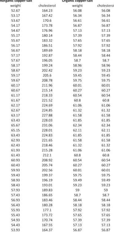
In order to alleviate the problem associated with consumption, an organic copper-salt combination was used instead of the inorganic com-binations currently used in preparation of poultry feeds. 96 chickens were randomly selected and randomly divided into two groups of 48
each. Each group was subjected to the same general conditions and treatments, differing only in that while, the chickens in the first group were fed with inorganic copper-salt, those in the second group were fed with inorganic copper-salt. After 4 Months the weight(gram) and cholesterol level(mg/egg) of the eggs yielded by the two groups were measured. The data are presented in the Appendix B.
Normality assumptions are common in data analysis, but a close look at the normal and generalized exponential power Q-Q plot in Figures 1 and 2 of Appendix A, though by the normal distribution is a reasonable fit, the tails seem to be shorter than expected and hence p-values resulting from the usual tests based on normal assumptions cannot be trusted. On the other hand, the generalized exponential power distribution proves to be a much better fit for egg weights as well as cholesterol level in both groups. We now carry out estimation of the parameters of the distribution using the method of moments and maximum likelihood estimate (MLE). These methods were preferred because they have many optimal properties in estimation: sufficiency; consistency; efficiency; and parameterization invariance which are rarely found in other approaches (For details on MLE see Spanos (1999) and Casella and Berger (2002)). The estimated values from the observations namely the means, standard deviation (s.d.), theω, Akaike information Criterion (AIC) as well as Bayesian Information criterion (BIC)are given in Table 1 with the corresponding log-likelihood (log(ℓ)) estimates. Since the explicit expression cannot be obtained for µand ω
in the estimation of maximum likelihood in the Section 2 we employed a numerical approach using a written code in the R software programme. The statistical computing environment (Ihaka & Gentlemen, 1996), was supplemented with the package called ”normp” downloaded into R file from the site http://cran.r-project.org/ and used to analyze the data. As earlier stated, though the normal distribution was a good fit to the sample data, but we have a better fit when we use the generalized exponential power distribution. This is evident when comparing the results form the log-likelihood functions, AIC and BIC given in Table 1 below, as well as the plots in figures 1 and 2.
T able 1: P arameters Estimation for eggs w eigh ts in App endix B densit y V ariables mean s.d shap e( ω ) h( ω ) log ( ℓ ) AIC BIC normal w eigh t(inorganic) 58.350 3.559 nil nil -129.055 262.11 273.5948 w eigh t(organic) 59.10 1.822 nil nil -96.910 197.82 209.3048 cholesterol(inorganic) 195.728 21.907 nil nil -216.282 436.564 448.0488 cholesterol(organic) 131.457 37.232 nil nil -241.739 487.478 498.9628 GEP w eigh t(inorganic) 58.507 4.371 4.470 0.281 -126.028 258.056 275.2832 w eigh t(organic) 59.118 2.306 5.963 0.168 -91.850 189.700 206.9272 cholesterol(inorganic) 194.481 28.359 6.825 0.147 -210.809 427.618 444.8452 cholesterol(organic) 129.720 46.327 5.206 0.192 -237.448 480.896 498.1232
4.1 Hypothesis Testing
We have used a numerical algorithm written in the R software envi-ronment to find estimates of the parameters giving the best fit for the data in appendix B. These estimates are reported in Table 1. We used the Kolmogorov-Smirnov two-sample test for large samples to decide whether there is significant difference in the weights and cholesterol lev-els of the two groups. Clearly, if we find that there is a significant difference, then feeds should be changed to organic copper-salts. Note that we have used a one sided Kolmogorov-Smirnov two-sample test i.e. the test compares the cumulative frequency distributions of the two samples and determines whether the observed D indicates that they have been drawn from different populations, one of which is stochasti-cally larger than the other. Let Fn1(X) be the cumulative step
func-tion of the sample observafunc-tions for the inorganic copper-salt type and let Fn2(Y) be the cumulative step function of the sample observations
for organic copper-salt type. We test the null hypothesis that the two samples have been drawn from the same population against the alter-native hypothesis that the values of the population from which one the samples was drawn are stochastically larger than the values of the pop-ulation from which the other sample was drawn. In other words, for the eggs weights the null and alternative hypotheses are of the form
H0 :Fn1(X) =Fn2(Y) and HA:Fn1(X)< Fn2(Y); also for the
choles-terol levels while the null hypothesis remain the same, the alternative hypothesis isHA:Fn2(X)< Fn1(Y). We now define
D=maximum[Fn1(X)−Fn2(Y)]
The sampling distribution of D is assumed to be a generalized ex-ponential power distribution. It has been shown by Goodman (1954) that
χ22 = 4D2n
2 (21)
(for number of observations are the same)
1. for the egg weightsD= 0.3125 with correspondingP[χ22 >9.21]<
0.01. Hence, we rejectH0and conclude that the weight of the eggs fed with inorganic copper salt is less than the organic type. 2. for the cholesterol level which is the most important, we have:
D = 0.6875 with P[χ22 > 45.375] < 0.0001. Hence we reject the the null hypothesis and conclude that, using the organic copper-salt type the cholesterol level significantly reduced.
5
Concluding Remarks
We have proposed a generalized exponential power distribution, and studied some of its mathematical and statistical properties. We fit-ted this distribution to data arising from an experiment concerning the cholesterol level and weight of eggs. The Q-Q plots clearly show that the generalized exponential power distribution fits the data better than the usual normal distribution. Finally, hypotheses tests show that con-sumption of eggs from chicken fed with organic copper-salt should not be boycotted for the fear of high cholesterol level. This assertion is further buttressed with the box plots in Figure 4 of Appendix A. Therefore we recommend that the constituents of poultry feeds should change from the inorganic to organic combinations.
Acknowledgments
I wish to express my sincere gratitude to the Authorities and Man-agements of Universita di Padova, Italy and the COIMBBRA group of universities for the opportunities availed to me during a three months fellowship at the University where part of this research was carried out under the advice of Prof. Adelchi Azzalini. I also thank Prof. Matthew Ojo of the Obafemi Awolowo University, Ile-Ife, Nigeria for his meaning-ful contributions. The very usemeaning-ful comments by the anonymous referee significantly improved the paper.
References
Box, G. E. P. (1953), A note on the Region of Kurtosis. Biometrika, 40, 465-468.
Cambanis, S., Huang, S., and Simons, G. (1981), On the Theory of Elliptically Contoured Distributions. J. Mult. Anal.,11, 368-85. Cassella and Berger (2002), Statistical Inference. Second edition,
Pa-cific Grove, CA: Duxberry.
Fang, K. T., Kotz, S., and Ng, K. W. (1990), Symmetric Multivariate and Related Distributions. London: Chapman and Hall.
Gradshteyn, I. S. and Ryzhik, I. M. (2007), Table of Integrals, Series and Products. 7th. Edition, 887-891, Academic Press.
Gomez, E., Gomez-Villegas, M. A., and Marin, J. M. (1998), A Multi-variate Generalization of the Power Exponential Family of Distri-butions. Communications in Statistics, Theory and Methods, 27, 589-600.
Goodman, L. A. (1954), Kolmogorov-Smirnov tests for Psychological Research. Pschol. Bull., 51, 160-168.
Ihaka, R., and Gentleman, R. (1996), A Language for Data Analysis and Graphics. Journal Computational and Graphical Statistics, 5, 299-314.
Kelker, D. (1971), Distribution theory of Spherical Distributions and a Location-Scale parameter. Sankhya, Ser. A,32, 419-30.
Lindsey, J. K. (1999), Multivariate Elliptically Contoured Distributions for Repeated Measurements. Biometrics, 55, 1277-1280.
Mahalanobis, P. C. (1930), On the generalized distance in statistics. Journal Asiat. Soc. Bengal, Vol. XXVI, 541-588.
Majumder, K. and Wu, J. (2009), Angiotensin I Converting Enzyme Inhibitory Peptides from Simulated in Vitro Gastrointestinal Di-gestion of Cooked Eggs. J. Agric. Food Chem.,52(2), 471-477. Spanos, A. (1999), Probability Theory and Statistical Inference.
Cam-bridge: Cambridge University Press.
Stewart Truswell, A. (2010), Cholesterol and Beyond: The Research on Diet and Coronary heart Disease 1900-2000. Springer Dordrecht Heidelberg London New York.
Subbotin, M. T. (1923), On the Law of Frequency of Error. Mathe-maticheskii Sbornik, 296-300.
Turner, M. E. (1960), On Heuristic Estimation Methods. Biometrics, 16, 299-401.
Vianelli, S. (1963), La Misura di Variabilita Condizionata in uno Schema Generalle delle Curve Normalli di Frequenza. Statistica, 23, 447-473.
Appendix A
Figure 3: Box plot of eggs weight for inorganic(1) and Organic (2) copper-salt combination
Figure 4: Box plot of eggs cholesterol contents for inorganic(1) and Organic (2) copper-salt combinations
Appendix B
Figure 5: Observed Data from Inorganic and Organic Copper-Salt