Sharif University of Technology
Scientia IranicaTransactions A: Civil Engineering http://scientiairanica.sharif.edu
Research Note
The application of multi-objective charged system
search algorithm for optimization problems
A. Ranjbar
a, S. Talatahari
b;, and F. Hakimpour
aa. Department of GIS Engineering, Faculty of Surveying Engineering, Tehran University, Tehran, Iran. b. Department of Civil Engineering, University of Tabriz, Tabriz, Iran.
Received 11 July 2017; accepted 16 February 2019
KEYWORDS Charged system search;
Meta-heuristics; Multi-objective optimization; Pareto optimal; Multi-objective charged system search.
Abstract. The charged system search algorithm is a relatively new optimization algorithm developed based on some principles from physics and mechanics. This paper presents an approach in which Pareto dominance is incorporated into the charged system search in order to allow this algorithm to handle problems with some multi-objective functions; the proposed algorithm will be called Multi-Objective Charged System Search (MOCSS). Well-known mathematical and engineering benchmarks were used to evaluate the proposed algorithm, and the results were compared with those of other new approaches. The results of implementing an algorithm on some test problems show that the proposed algorithm outperforms other algorithms in terms of generational distance, maximum spread, spacing, coverage of two sets, and hypervolume indicator. Results of well-known mathematical examples indicate that an approach is highly competitive and can be considered as a viable alternative to solving multi-objective optimization problems. These results encourage the application of the proposed method to more complex and real-world multi-objective optimization problems. The proposed method can deal with highly nonlinear problems with complex constraints and diverse Pareto optimal sets.
© 2019 Sharif University of Technology. All rights reserved.
1. Introduction
Many realistic problems contain simultaneous opti-mization of several objectives that may conict with each other and with other nonlinear constraints, if available [1-7]. These types of problems are known as Multi-Objective Problems (MOPs). Multi-objective optimization (also known as vector optimization, multi-criteria/attribute optimization, multi-objective pro-gramming, or Pareto optimization) is dened as the process of nding a decision vector to optimize a set of objective functions that satises some certain *. Corresponding author.
E-mail address: [email protected] (S. Talatahari) doi: 10.24200/sci.2018.20184
constraints [8,9], while the aim of single-objective optimization is to optimize just one objective func-tion. In contrast with a single-objective optimization, multi-objective problems are more dicult and com-plex [10,11]. Some reasons for this are as follows:
1. In single-objective optimization, the tness of so-lutions is reachable easily due to the existence of just one objective function, while no single unique solution can be determined as the best for multi-objective optimization; instead, a set of non-dominated solutions should be found in order to obtain a good approximation of the true Pareto fronts [3,12-14], leading to a trade-o among the objectives [15,16];
2. Algorithms that work well for single-objective prob-lems usually cannot directly be used for
multi-objective ones, and it is necessary to consider some special conditions. As a simple way, one can combine multiple objectives into a single objective using some weighted sum method [17];
3. Even if a multi-objective algorithm can nd so-lutions on a Pareto front, there is no guarantee that distribution of multiple Pareto points becomes uniform, and this may reduce the applicability of the results [3,14,17].
Therefore, developing an ecient multi-objective algorithm for solving multi-objective optimization problems seems inevitable.
Nowadays, Multi-Objective Evolutionary Algo-rithms (MOEAs) have shown an acceptable perfor-mance in many benchmarks and real-world problems with their origins in engineering, scientic, and in-dustrial areas [1]. The main reason for the pop-ularity of evolutionary algorithms for solving multi-objective optimization is their population-based nature and ability to nd multiple optima simultaneously. In 1985, Schaer was probably the rst to use Vector Evaluated Genetic Algorithms (VEGA) to solve multi-objective optimization without using any composite aggregation and by combining all objectives into a single objective [18]. After that, a wide variety of MOEAs have been suggested such as Micro-Genetic Algorithm (Micro-GA) [19], Non-dominated Sorting Genetic Algorithm (NSGA) [20], new variant of NSGA or NSGA-II [21], Strength Pareto Evolutionary Al-gorithm (SPEA) [22], SPEA2 [23], Pareto Archive Evolution Strategy (PAES) [24], Pareto Dierential Evolution Approach (PDEA) [25], MOEA/D: A Multi-Objective Evolutionary Algorithm based on Decom-position [26], NSGAII based on Dierential Evolution (NSGAII-DE [27]), a hybrid multi-objective particle swarm optimization and decision-making procedure for optimal design of truss structures [28], the third version of Generalized Dierential Evolution (GDE3) [29], Multi-Objective Dierential Evolution-the Ranking-based Mutation Operator (MODE-RMO) [30], Multi-Objective Particle Swarm Optimization (MOPSO) [31], Dierential Evolution for Multi-objective Optimization (DEMO) [32], a novel hybrid charged system search and particle swarm optimization method for multi-objective optimization [33], Multi-Objective Dieren-tial Evolution (MODE)[34], multi-objective bees al-gorithms (Bees) [35], and Non-dominated Rank Ge-netic Algorithm (NRGA) [36]. In recent years, some other types of algorithms have also been developed such as Multi-Objective Cuckoo Search (MOCS) [37], Multi-Objective Firey Algorithm (MOFA) [38], a new multi-swarm multi-objective optimization method for structural design [39], a swarm-based memetic evolu-tionary algorithm for multi-objective optimization of large structures [40], Multi-Objective Flower
Pollina-tion Algorithms (MOFPA) [17], and multi-objective optimization method based on sensitivity analysis [14]. Regardless of the number of these methods and their dierences, they share some defections as follows:
I. The nal distribution of Pareto points is not often well-spread; therefore, maximum information on the Pareto cannot often be obtained [13,41];
II. The nding results often require heavy computa-tion and are time consuming.
Therefore, the development of a new multi-objective optimization method to resolve some of these drawbacks seems necessary.
Kaveh and Laknejadi (2011) [33] used a hy-brid charged system search and particle swarm multi-objective optimization, where the answers space was divided based to some spaces in order to nd a uni-form Pareto point. A multi-objective charged system search was developed by Kaveh and Massoudi [42]. These algorithms are extended to the single-objective Charged System Search (CSS), as introduced by Kaveh and Talatahari [43,44].
In the present paper, another variant of Multi-Objective Charged System Search (MOCSS) is pre-sented, where the idea of the non-dominated method is used.
The rest of the paper is organized as follows. Section 2 describes the basic characteristics of the standard CSS. In Section 3, the multi-objective CSS algorithm will be presented in detail. The fundamental concept of the utilized constraint-handling method for MOCSS in detail is described in Section 4. The bench-mark function, multi-objective performance metrics, and computational results are presented in Section 5. Validation of the MOCSS by some engineering design problems will be presented in Section 6. Finally, some relevant issues, future works, and conclusions are drawn in Section 7.
2. A brief review on standard charged system search
In physics, the electric eld around an electric charge is the space surrounding it and applies a force to other electrically charged objects. The Coulomb law deter-mines the electric eld surrounding a point charge. Its value is proportional with the product of two charged particles and inversely square of the separation distance between the particles directed along the line. Based on Gauss's law, the magnitude of the electric eld at a point inside a charged sphere can be determined (proportional with the separation distance between the particles). By using these principles, the standard Charged System Search (CSS) denes a number of solution candidates or Charged Particles (CPs) that
act as a charged sphere and can apply electrical forces to the other CPs. The resultant force acts on each CP creating acceleration, according to Newton's second law. Finally, by utilizing the Newtonian mechanics, the position of each CP is determined at any time based on its previous position, velocity, and acceleration in the search space [43]. The main formula of electrical physics for calculating the electrical force between two CPs is as follows:
Fj= qj
X
i;i6=j
(aqi3rij:i1+rqi
ij2:i2)pij(Xi Xj);
8 < :
j = 1; 2; :::; n
i1= 1; i2= 0 , rij< a
i1= 0; i2= 1 , rij a
(1) where:
a The radius of the charged sphere; n The total number of CPs;
Fj The resultant force acting on the jth
CP;
qi The magnitude of the charge;
rij The separation distance between two
charged particles;
pij The probability of two charged
particles;
Xi and Xj The positions of the ith and jth CPs.
The initial position of CPs is obtained through Eq. (2) in the search space:
xi;j = xi;min+ rand (xi;max xi;min);
i = 1; 2; :::; n; (2)
where xi;j determines the initial value of the ith
vari-able for the jth CP; xi;minand xi;maxare the minimum
and the maximum allowable values for the ith variable; rand is a random number at the interval [0,1]; and n is the number of variables. The magnitude of the charge is calculated by the quality of solutions as follows:
qi=fit(best) fit(worst)fit(i) fit(worst) ; i = 1; 2; :::; n; (3)
where fit(best) and fit(worst) are the best and the worst tness of all particles so far; fit(i) represents the objective function value or the tness of agent i; n is the total number of CPs. In Eq. (4), a force is attractive as long as all good CPs can attract bad CPs and only some of bad agents attract good agents due to appropriate exploitation and exploration abilities as follows:
pij = (
1 fit(i) fit(best)fit(j) fit(i) > rand or fit(j) > fit(i)
0 else (4)
The separation distance, rij, between two charged
particles is also dened as follows: rij= kXi Xjk
(Xi+Xj)
2 Xbest + "
; (5)
where Xi and Xj are the positions of the ith and jth
CPs, Xbest is the position of the best current CP, and
" is a small positive number to avoid singularities. The radius of the charged sphere (a) is considered as follows: a = 0:1 max(fxi;max xi;minji = 1; 2; :::; ng): (6)
Further, the main formula of the CSS uses New-ton's laws (with some modications) for calculating the new position and velocity of each CP as follows:
Xj;new= 0:5randj1:(1 + iteriter max)
:X
i;i6=j
(aq3irij:i1+rqi
ij2:i2)pij(Xi Xj)
+ 0:5randj2:(1 iteriter
max):Vj;old+ Xj;old(7);
Vj;new= Xj;new Xj;old; (8)
where iter is the actual number of iterations, and itermax is the maximum number of iterations.
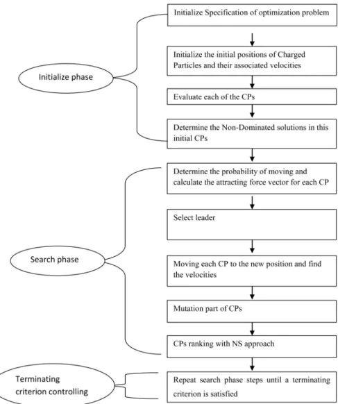
3. Multi-objective charged system search The proposal optimization algorithm, so-called Multi-Objective Charged System Search (MOCSS), is used for solving multi-objective problems by combining CSS algorithm with Non-dominated Sorting (NS) for good convergence and high diversity of Pareto front [45], respectively. NS sorts the solutions on the basis of non-domination and, then, forms the levels of Pareto fronts. For selecting the numbers of the best solution, the solutions with the highest Pareto front rank are chosen; if required, the other solutions are selected for the next Pareto front. This process is repeated until the Crowding Distance (CD) condition is satised (according to Figure 1). This article utilized the mutation function from GA in order to prevent early convergence. The following pseudo-codes summarized the MOCSS algorithm:
Level 1: Initialization
Step 1: Initialize specication of the optimization problem and algorithm parameters;
Step 2: Initialize the rst positions of charged particles and their associated velocities;
Figure 1. Flow diagram that shows the way in which the NS works. P (t) is the population at generation t; F 1 is the best solution; and F 2 is the second best solutions, and so on (Coello et al., p. 94, 2007) [4].
Step 3: Evaluate all CPs;
Step 4: Determine the non-dominated solutions for the initial CPs.
Level 2: Search
Step 1: Determine the probability of moving and calculate the attracting force vector for each CP; Step 2: Select the leader;
Step 3: Move each CP to the new position and nd their velocities;
Step 4: Mutate some CPs;
Step 5: Rank CPs according to the NS approach. Level 3: Terminating criterion controlling Repeat search level steps until a terminating criterion is satised
The owchart of the MOCSS algorithm is illus-trated in Figure 2.
4. Constraint-handling method for the MOCSS
Consider the general form of a constrained multi-objective optimization problem [46,47] as follows: Find x that minimizes
F (x) = (f1(x); :::; fk(x)); (9)
subject to:
G(x) = (g1(x); :::; gh(x)) 0; (10)
where x = (x1; :::; xnV ar) is the vector of solution that
minimizes objective function(s) F (x) while satisfying constraint(s) G(x) 0. The number of design parameter(s), objective function(s), and constraint(s) are denoted by nV ar, k, and h, respectively.
Multi-Objective Evolutionary Algorithms (MOEAs) are robust and ecient multi-objective optimization algorithms; however, EAs do not have any explicit mechanism to handle constraints, while most real-world design multi-objective optimization problems have multiple constraints [48]. The penalty function method is a traditional approach to handling the constraints of single-objective optimization problems. However, this method requires careful tuning of the penalty function coecients to obtain a satisfactory design. Moreover, the application of this method to a multi-objective optimization problem raises another problem: How to combine multiple constraints with multiple objectives [11,48].
Many previous constraint-handling methods need to tune some parameters to make a balance between the objective(s) and constraint(s). This study uses a constraint-handling method proposed by Oyama (2007) [48], which does not need any parameters to be tuned for constraint handling and it can always be used
Figure 2. The ow-chart of MOCSS algorithm.
even when all individuals in the initial population are infeasible, or the amount of violation of each constraint is signicantly dierent. The method is described in the following.
Denition 1 (constrained Pareto dominance): Solution i is said to constrained-dominate solution j if any of the following conditions are true:
1. Solutions i and j are both feasible, and solution i dominates solution j in the objective function space. It should be noted that solution xi is said
to dominate solution xj if fk(xi) is no worse than
fx(xj) for all objectives, and it is better for at least
one of them [21,49]:
fk(xi) fk(xj); 8i = 1; 2; :::; k
fk(xi) < fk(xj); 9i 2 f1; 2; :::; kg: (11)
Thus, a set of solutions is said to be a Pareto front or Pareto solution if no element of this set dominates any other solutions [50]. For more details on Pareto optimal solutions, one can be referred to [31,51].
2. Solution i is feasible and solution j is not.
3. Solutions i and j are both infeasible; yet, solution i dominates solution j in the constraint space. Denition 2 (constraint space dominance): Solution i is said to dominate solution j in the con-strained space if both of the following conditions are true:
1. Solutions i is not worse than solution j in all constraints, i.e.:
2. Solution i is strictly better than solution j for at least one constraint, i.e.:
8Gn(xi) < Gn(xj); (13)
where:
Gn(x) = max(0; gn(x)); n = 1; 2; :::; k: (14)
By means of Oyama's constraint-handling ap-proach, niching based on the number of constraint violations was applied to infeasible solutions. Here, a standard tness sharing [52] was applied to infeasible designs based on their constraint violations as follows:
rank0(x
i) = rank(xi) P enalty(xi);
P enalty(xi) = 1 + npopX j=1;j6=i
shij;
shij =
(
1 dij
share
dij<share
0 dij share
share= h
X
n=1
(gmaxn gminn )=npop;
dij =
v u u tXh
n=1
(gn(xi) gn(xj))2;
gmaxn= max(fgn(x1); :::; gn(xnpop)g);
gminn = min(fgn(x1); :::; gn(xnpop)g); (15)
where npop is population size and is set to 0.4. 5. Numerical investigation
5.1. Benchmark problems
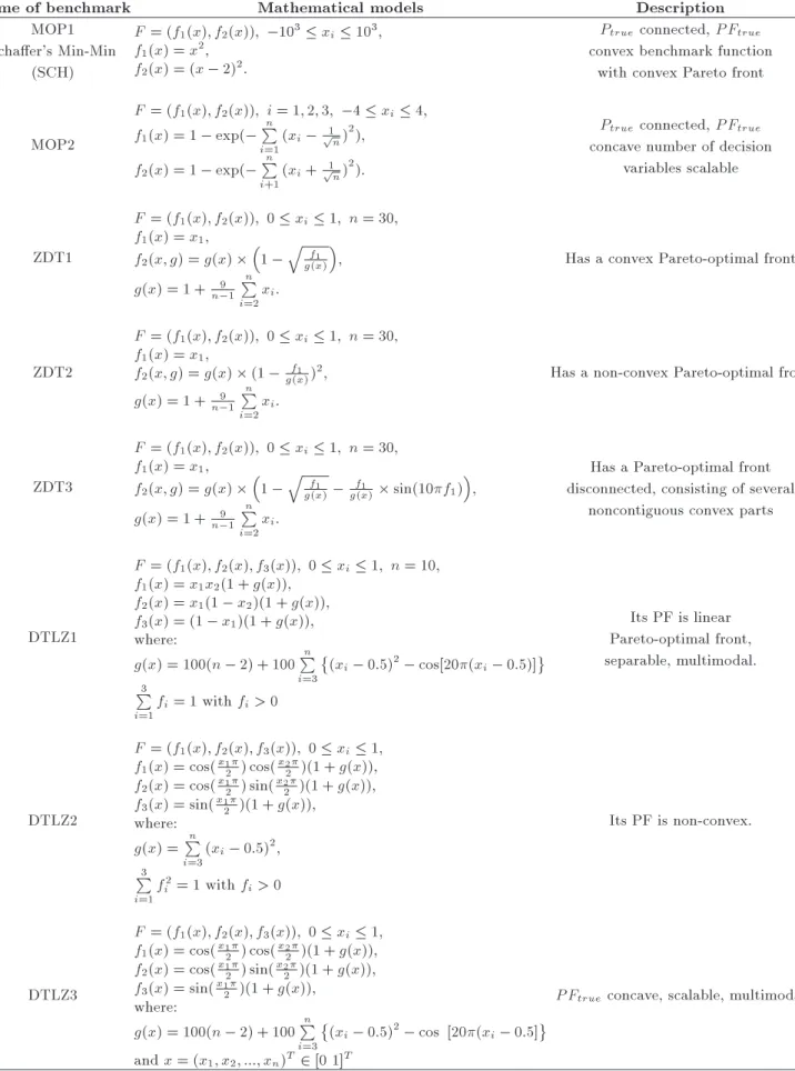
There are many dierent multi-objective benchmark functions for evaluating the performance of algo-rithms [22,37,53]. In this paper, for validating the MOCSS, ten of these functions have been selected containing convex (ZDT1 [8] and MOP1 [18]), non-convex (ZDT2 and MOP2 [8,13,54]), and discontinuous Pareto fronts with more complex Pareto set problems (ZDT3 [8], DTLZ1, DTLZ2, DTLZ3, DTLZ4, and DTLZ5 test functions [55]). Table 1 presents the details of these examples.
5.2. Multi-objective performance metrics To evaluate the performance of multi-objective op-timization algorithms, a general approach is utilized to compare quantitative results [13,56] or the amount of relative distribution on the Pareto front for test functions [37]. In order to determine a quantitative
assessment of the performance of a multi-objective optimization algorithm, three issues are normally taken into consideration [57]:
I) The distance of the Pareto front produced by an algorithm with respect to the real Pareto front;
II) The spread of solutions found;
III) The number of elements of the Pareto optimal set found.
For the rst two, small values are better than the larger one, while the number of elements of the Pareto optimal set should be maximized for the last one.
In order to compare the results of dierent MOP problems, dierent performance metrics are usually utilized in the literature [31]; the following subsections describe these metrics.
I. Generational Distance (GD). The concept of generational distance was introduced by Van Veldhuizen and Lamont [13,54,58] for estimating how far the elements are in the set of generated Pareto fronts so far from those in the Pareto front true, and it is dened as follows:
GD = s
n
P
i=1d 2 i
n ; (16)
where n is the number of so far solutions in P Fknown, and di is the Euclidean distance of the
objective space between each of solutions and the nearest member of the true Pareto front. It should be noted that a value of GD = 0 indicates that all the generated elements are in the true Pareto front, i.e., P Ftrue = P Fknown. Therefore, any
other value indicates how \far" we are from the global Pareto front of our problem. This metric needs to know P Ftrue;
II. Maximum Spread (MS). The metric of Maxi-mum Spread (MS) measures how \well" P Ftrueis
covered by P Fknown through hyper-boxes formed
by the extreme function values observed in P Ftrue
and P Fknown. It is dened as shown in Box I:
where m is the number of objectives, fmax i , fimin,
Fmax
i , and Fimin are the maximum and minimum
of the ith objective in P Fknown and P Ftrue,
respectively. A larger value of MS implies better spread of solutions. In this study, Fmax
i and Fimin
are considered as the maximum and minimum of the ith objective in all the Pareto fronts obtained by various algorithms [49]. This metric needs to know P Ftrue;
III. Spacing (S). The Spacing (S) metric numer-ically describes the spread of the vectors in
Table 1. Benchmark for multi-objective optimization.
Name of benchmark Mathematical models Description
MOP1 Schaer's Min-Min
(SCH)
F = (f1(x); f2(x)); 103 xi 103,
f1(x) = x2,
f2(x) = (x 2)2:
Ptrueconnected, P Ftrue
convex benchmark function with convex Pareto front
MOP2
F = (f1(x); f2(x)); i = 1; 2; 3; 4 xi 4,
f1(x) = 1 exp( n
P
i=1(xi 1 pn)2),
f2(x) = 1 exp( n
P
i+1(xi+ 1 pn)2):
Ptrueconnected, P Ftrue
concave number of decision variables scalable
ZDT1
F = (f1(x); f2(x)); 0 xi 1; n = 30,
f1(x) = x1,
f2(x; g) = g(x)
1 q f1
g(x)
, g(x) = 1 + 9
n 1 n
P
i=2xi:
Has a convex Pareto-optimal front
ZDT2
F = (f1(x); f2(x)); 0 xi 1; n = 30,
f1(x) = x1,
f2(x; g) = g(x) (1 g(x)f1 )2,
g(x) = 1 + 9 n 1
n
P
i=2xi:
Has a non-convex Pareto-optimal front
ZDT3
F = (f1(x); f2(x)); 0 xi 1; n = 30,
f1(x) = x1,
f2(x; g) = g(x)
1 q f1
g(x) g(x)f1 sin(10f1)
, g(x) = 1 + 9
n 1 n
P
i=2xi:
Has a Pareto-optimal front disconnected, consisting of several
noncontiguous convex parts
DTLZ1
F = (f1(x); f2(x); f3(x)); 0 xi 1; n = 10,
f1(x) = x1x2(1 + g(x)),
f2(x) = x1(1 x2)(1 + g(x)),
f3(x) = (1 x1)(1 + g(x)),
where:
g(x) = 100(n 2) + 100Pn
i=3
(xi 0:5)2 cos[20(xi 0:5)] 3
P
i=1fi= 1 with fi> 0
Its PF is linear Pareto-optimal front, separable, multimodal.
DTLZ2
F = (f1(x); f2(x); f3(x)); 0 xi 1,
f1(x) = cos(x12) cos(x22)(1 + g(x)),
f2(x) = cos(x12) sin(x22)(1 + g(x)),
f3(x) = sin(x12)(1 + g(x)),
where: g(x) =Pn
i=3(xi 0:5) 2, 3
P
i=1f 2
i = 1 with fi> 0
Its PF is non-convex.
DTLZ3
F = (f1(x); f2(x); f3(x)); 0 xi 1,
f1(x) = cos(x12) cos(x22)(1 + g(x)),
f2(x) = cos(x12) sin(x22)(1 + g(x)),
f3(x) = sin(x12)(1 + g(x)),
where:
g(x) = 100(n 2) + 100Pn
i=3
(xi 0:5)2 cos [20(xi 0:5]
and x = (x1; x2; :::; xn)T 2 [0 1]T
Table 1. Benchmark for multi-objective optimization (continued).
Name of benchmark Mathematical models Description
DTLZ4
F = (f1(x); f2(x); f3(x)); 0 xi 1,
f1(x) = cos(x12) cos(x22)(1 + g(x)),
f2(x) = cos(x12) sin(x22)(1 + g(x)),
f3(x) = sin(x12)(1 + g(x)),
where: g(x) =Pn
i=3(xi 0:5)
2; = 100
and x = (x1; x2; :::; xn)T 2 [0 1]T
P Ftrueconcave, separable, unimodal.
DTLZ5
F = (f1(x); f2(x); f3(x)); 0 xi 1,
f1(x) = cos(12) cos(22)(1 + g(x)),
f2(x) = cos(12) sin(22)(1 + g(x)),
f3(x) = sin(12)(1 + g(x)),
where: g(x) =Pn
i=3(xi 0:5) 2
1= x1; 2=(1+2x2(1+g(x))2;g(x)) and x = (x1; x2; :::; xn)T 2 [0 1]T
P Ftrueunimodal
The function value of a Pareto optimal
solution satises
3
P
i=1f 2 i = 1
MS = "
1 m
m
X
i=1
min(fmax
i ; Fimax) max(fimin; Fimin)
Fmax
i Fimin
2#12
: (17)
Box I
P Fknown [33,59]. This Pareto front metric
mea-sures the distance variance of neighboring vectors in P Fknown. Eqs. (18) and (19) dene this metric:
S = "
1 n 1
n
X
i=1
(di d)2 #1
2
where d =
n
P
i=1di
n(18); di=minj f1i(!x ) f1j(!x )+f2i(!x ) f2j(!x )
; i; j = 1; 2; :::; n; i 6= j; (19) where n is the number of vectors in P Fknown.
When S = 0, all members are spaced evenly apart. Note that this becomes important in the deception problems where all Pareto front vectors are equally spaced. This metric does not require the user to know P Ftrue;
IV. Coverage of two set (CS). In order to compare the dominant relationship between two popula-tions resulting from two dierent MOEAs, Zitzler et al. [2003] proposed the CS [56] that is measured to show how the nal population of one algorithm dominates the nal population of another algo-rithm. Eq. (20) denes this metric:
CS(X0; X00) = jfa002 X00; 9a0 2 X0 : a0 a00gj
jX00j ;
(20) where X0 and X00 are two sets of solutions
re-sulting from dierent algorithms, where a0 a00
means that a0 dominates a00 if and only if a0 < a00
or a0= a00. Function CS is dened as the mapping
of the order pair (X0; X00) to the interval [0,1].
In general, if all solutions in X0 dominate all
solutions in X00, then CS(X0; X00) = 1. In
addition, CS(X0; X00) = 0 implies that none of
the solutions in X00 is dominated. Note that
both CS(X0; X00) and CS(X00; X0) need to be
considered independently since they have distinct meanings and CS(X0; X00) is not necessarily equal
to 1 CS(X00; X0). The advantage of this Pareto
compliant metric is that it is easy to calculate and provide a relative comparison based on dominant numbers between two MOEAs [57];
V. Hypervolume indicator of set S. Let the ref-erence point be denoted by Ref = (r1; r2; :::; rk).
The hypervolume indicator of S (denoted as Hv(S)) is dened as the volume of the hypercube restricted by all points in S and Ref.
Hv(S) = Leb( [
~x2Sjf1(~x1); r1j
f2(~x2);
r2
::: jfk(~xk); rkj)); (21)
where k is the number of dimensions, Leb(S) indi-cates the Lebesgue measure of S, and jf1(~x1); r1j
jf2(~x2); r2j ::: jfk(~xk); rkj represents the
hy-percube formed by points, dominated by ~x as Ref. [60].
5.3. Numerical results
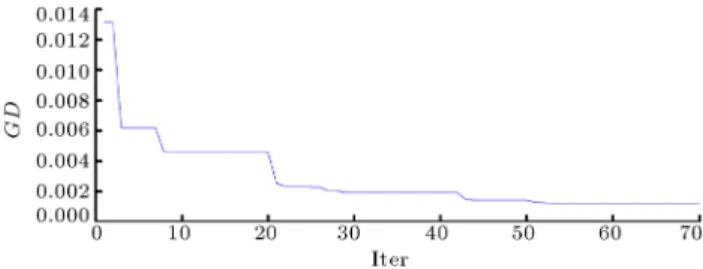
For the MOP 1 example, Figure 3 shows the exponential-like decrease of GD as the iterations pro-ceed. Clearly, it can be seen that the MOCSS algorithm indeed converges almost exponentially. The estimated Pareto fronts and true Pareto fronts of other functions
Figure 3. Convergence of the proposed MOCSS. The least-square distance (vertical axis) from the estimated front to the true front of MOP1 for the rst 70 iterations (horizontal axis).
are shown in Figure 4. In all of these gures, the horizontal axis is the rst objective function, and the vertical axis is the second one. The gure shows that the MOCSS algorithm is able to nd proper solutions for the benchmark examples. Further, the solutions are scattered among the Pareto fronts identically. Therefore, this algorithm is able to correctly obtain the Pareto front.
A careful scrutiny of Figure 4 indicates that the proposed MOCSS algorithm for nding solutions has outperformed all benchmarks. The answers that are close to the true Pareto front, uniformly dispersed on it, should be found. The performances of the proposed multi-objective approach are evaluated based on the multi-objective metrics in terms of GD, S, and MS. The results are summarized in Tables 2(a) to 2(c), (including Mean, standard deviation, Best, and Worst with 30 independent runs). In all benchmark functions, the values of GD and S are close to zero, and the value of MS is close to one. This means that the result of MS metric shows that the MOCSS approach has better covered P Fknown, and the result of S metric shows that
MOCSS approach has better spread of the answer. In order to evaluate and compare the perfor-mances of the MOCSS with those of the other multi-objective optimization algorithms, the results of NSGA-II, VEGA, MODE, SPEA, Bees, DEMO, PDEA, MOEA/D. SPEA2, GDE3, NSGAII-DE, MODE-RMO, and MOFA are presented in Table 3. All results have been averaged over 30 independent runs.
Table 2(a). Results of the GD for the benchmarks (with 30 independent runs).
GD metric MOP1 ZDT1 ZDT2 ZDT3
Mean 0.00136 0.000178 0.000148 0.0007938 Standard deviation 0.00013 0.000037 0.000012 0.0001043 Best 0.00110 0.000110 0.000123 0.000640 Worst 0.00170 0.000274 0.000164 0.000977 Table 2(b). Results of the MS for the benchmarks (with 30 independent runs).
MS metric MOP1 ZDT1 ZDT2 ZDT3
Mean 0. 9934 1 0.9993 0.9591
Standard deviation 0.0109 1 0.0032 0.0783
Best 1 1 1 1
Worst 0.9596 1 0.9859 0.7924
Table 2(c). Results of the S for the benchmarks (with 30 independent runs).
S metric MOP1 ZDT1 ZDT2 ZDT3
Mean 0.0463 0.0126 0.0138 0.0268 Standard deviation 0.0143 0.0026 0.0025 0.0102 Best 0.0272 0.0087 0.0108 0.0104 Worst 0.0969 0.229 0.0217 0.0533
Figure 4. Pareto front of test functions: (a) MOP2, (b) MOP1, (c) ZDT1, (d) ZDT2, (e) ZDT3, (f) DTLZ1, and (g) DTLZ2.
In this table, results with Boldface indicate a better value. It can be seen that the MOCSS is one of the top best algorithms in nding optimum results.
5.4. Comparison study
In this section, the performance of the proposed MOCSS is compared with those of other established multi-objective algorithms, including Vector Evaluated Genetic Algorithm (VEGA), Non-dominated Sorting Genetic Algorithm II (NSGA-II), Multi-Objective Dif-ferential Evolution (MODE), Dierential Evolution
for Multi-Objective Optimization (DEMO), multi-objective Bees algorithms (Bees), Strength Pareto Evo-lutionary Algorithm (SPEA) and Multi-objective Fire-y Algorithm (MOFA), Strength Pareto EvolutionarFire-y Algorithm (SPEA2), Multi-Objective Evolution Algo-rithms with the Tchebyche approach (MOEA/D), Pareto Dierential Evolution Approach (PDEA), NS-GAII based on Dierential Evolution (NSNS-GAII-DE), the third version of Generalized Dierential Evolution (GDE3), and Multi-Objective Dierential Evolution-the Ranking-based Mutation Operator (MODE-RMO).
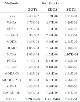
Table 3. Comparison of GD for n = 50 (charges particle) and iteration = 500, as presented in Refs. [30,37,25]. All results have been averaged over 30 independent runs. A result with Boldface indicates better value obtained.
Methods Test function
ZDT1 ZDT2 ZDT3
Bees 2.40E-02 1.69E-02 1.91E-01 VEGA 3.79E-02 2.37E-03 3.29E-01 SPEA 1.78E-03 1.34E-03 4.75E-02 NSGA-II 3.33E-02 7.24E-02 1.14E-01 MODE 5.80E-03 5.50E-03 2.15E-02 DEMO 1.08E-03 7.55E-04 1.18E-03 MOFA 1.90E-04 1.52E-04 1.97E-04 PDEA 6.15E-04 6.52E-04 5.63E-04 SPEA2 3.40E-03 9.10E-03 1.80E-03 MOEA/D 9.59E-04 5.81E-04 1.73E-03 MODE-RMO 3.85E-03 6.97E-03 4.76E-03 GDE3 2.40E-03 8.20E-03 2.76E-03 NSGAII-DE 5.83E-03 7.75E-03 5.31E-03 MOCSS 1.78 E-04 1.48 E-04 7.94E-04
The performances of the proposed multi-objective approach are evaluated and compared using the multi-objective metric in terms of GD (how far the known Pareto front is from the true Pareto front) with the above-mentioned MO approach given in Table 3. Overall, the MOCSS has better performance than the other thirteen cases, and it has the best convergence in ZDT1, ZDT2, and ZDT3 (except MOFA and PDEA) benchmark functions.
To check if the nal results obtained with the best performing algorithm dier from the nal results of the rest of the competing algorithms in a statistically signicant manner, the Wilcoxon's Ranksum test for independent samples [61] is used at a signicance level of 5%, as presented in Table 4. The numerical values of 1, 0, 1 correspond to whether the other methods are inferior to, equal to, and superior to our proposed algorithm, as indicated in Table 4.
The MOCSS is implemented and compared with NSGA-II and MOEA/D using DTLZ1 and DTLZ2 test functions in the coverage of two set metrics. Table 5 shows the coverage of two set metric values of the three approaches, averaged on 30 independent runs. A careful inspection of Tables 5 reveals that, in terms of coverage of two set metrics, the nal solutions obtained by the MOCSS are better than those obtained by
Table 4. Comparison between MOCSS and other algorithms on the basis of Wilcoxon's Ranksum test.
Methods Test function
ZDT1 ZDT2 ZDT3
Bees 1 1 1
VEGA 1 1 1
SPEA 1 1 1
NSGA-II 1 1 1
MODE 1 1 1
DEMO 1 1 1
MOFA 1 1 +1
PDEA 1 1 0
SPEA2 1 1 1
MOEA/D 1 1 1
MODE-RMO 1 1 1
GDE3 1 1 1
NSGAII-DE 1 1 1
1: worse;+1: better; and0: equal.
NSGA-II and MOEA/D for DTLZ1 and DTLZ2 test instances.
The Hypervolume indicator is employed to guide the diversity preservation in our approach. The ref-erence points used for assessments are r = 1:1d and
r = 1:1d for DTLZ1 and DTLZ2, respectively. Table 6
presents average and standard deviation relative hyper-volume for MOCSS, NSGA-II, and SPEA2 approaches. A larger hypervolume value is preferable when com-paring the performances of dierent solution sets. Therefore, the MOCSS approach performs signicantly better than the other two approaches. The results of GD obtained by GDE3, MODE-RMO, NSGAII-DE, and MOCSS, besides Wilcoxon's Ranksum test, are presented in Table 7. According to Table 7, the MOCSS outperforms NSGAII-DE in 4 problems and performs evenly in 1 problem. In addition, it outper-forms GDE3 in 3 problems and loses in 2 problems. It also outperforms MODE-RMO in 2 problems, loses in 2 problems, and performs evenly in 1 problems. Briey, for the tri-objective test functions, the MOCSS has better GD value in DTLZ1, DTLZ2, and DTLZ3 than another approach.
Finally, times were also evaluated (using the same hardware platform and the exact same environment for each of the two algorithms) in order to establish if our MOCSS algorithm was really faster than the NSGA-II or not. Table 8 shows that NSGA-II covers the entire Pareto front and is faster in computational time by 5 to 13 percent (on average 4 percent) than the MOCSS
Table 5. Average coverage of two set metrics between MOCSS, NSGA-II, and MOPSO (pop. = 50 and independent runs = 30).
Approach MOCSS MOEA/D NSGA-II
NSGA-II MOEA/D MOCSS NSGA-II MOCSS MOEA/D
DTLZ1 0.091 0.051 0.018 0.078 0.011 0.005
DTLZ2 0.072 0.048 0.028 0.099 0.016 0.001
in this test function. However, the implementation of the MOCSS method produces excellent results, as shown in Table 3.
6. Engineering design problem 6.1. Welded beam design
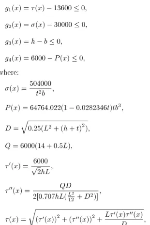
The design of a welded beam is a classical benchmark that has been solved by many researchers. The welded beam design is a real-life application problem [11,62], whose aim is to minimize the cost and the endpoint's deection subject to constraints on shear stress, bending stress, and buckling load (Figure 5). The detailed formulation can be found in [11,45,62,63].
Table 6. Average and standard deviation relative hypervolume among MOCSS, NSGA-II, and SPEA2 (independent runs = 30) [46].
Method DTLZ1, r = 0:7d DTLZ2, r = 1:1d
NSGA-II 0.94333 (0.11423) 0.86913(0.00803) SPEA2 0.98010(0.00152) 0.90760(0.00350) MOCSS 0.96201(0.01067) 0.92056(0.01538)
Figure 5. The welded beam design problem.
It is desired to nd four design parameters (thickness b, width t, length of weld L, and weld thickness h) for which the cost function of the beam and the deection function at the open end are objective functions [45]:
min f1(x) = 1:1047h2L + 0:0481tb(14 + t);
min f2(x) = (x) = 2:1952t3b ; (22)
subject to:
Table 7. Comparison between MOCSS and other algorithms on average GD metrics and the basis of Wilcoxon's Ranksum test [30] (independent runs = 20 and pop. = 100).
Example MOCSS GDE3 MODE-RMO NSGAII-DE
DTLZ1 2.72E-04 7.08E-02 1 2.58E-04 0 4.80E-03 1
DTLZ2 4.59E-04 7.25E-04 1 7.28E-04 1 1.96E-03 1 DTLZ3 6.59E-04 3.27E+00 1 7.88E-03 1 1.82E-01 1 DTLZ4 5.24E-04 7.12E-04 +1 7.26E-04 +1 1.46E-03 1
DTLZ5 1.93E-04 1.09E-05 +1 9.12E-06 +1 1.87E-04 0
1: worse;+1: better; and0: equal.
Table 8. Average and Standard deviation computational time between MOCSS and NSGA-II (independent runs = 30). Test function
MOCSS NSGA-II
Pop.= 50 and Iter.=50
Pop.=100 and Iter.=100
Pop.=50 and Iter.=50
Pop.=100 and Iter.=100 MOP1 31:05 0:31 218:75 1:53 30:11 0:56 217:19 1:31
ZDT1 28:46 0:28 192:46 2:34 24:85 1:13 187:67 2:03 ZDT2 28:72 0:27 192:23 2:34 25:28 0:99 186:16 3:36 ZDT3 28:36 0:34 191:35 0:96 27:36 1:01 202:53 1:21
g1(x) = (x) 13600 0;
g2(x) = (x) 30000 0;
g3(x) = h b 0;
g4(x) = 6000 P (x) 0;
where:
(x) = 504000t2b ;
P (x) = 64764:022(1 0:0282346t)tb3;
D = q
0:25(L2+ (h + t)2);
Q = 6000(14 + 0:5L); 0(x) = p6000
2hL;
00(x) = QD
2[0:707hL(L2
12 + D2)]
; (x) =
r
(0(x))2+ (00(x))2+L0(x)00(x)
D ;
where the simple limits for variables are 0:1 L, t 10 and 0:125 h, b 5.
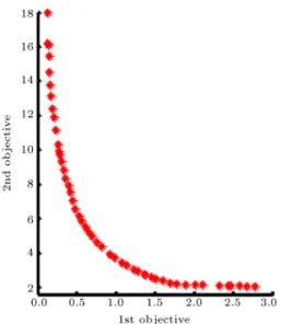
In the welded beam design problem, the non-linear constraints can cause diculties in nding the Pareto front. This design problem has been solved by the MOCSS. The Pareto front of 50 solution points after 1000 iterations is obtained by the MOCSS, as shown in Figure 6. The obtained results include distribution, spread, and smoothening, which are the same with or better than the results obtained in other researches [11,45,62].
Figure 6. Pareto front for the bi-objective beam design where the horizontal axis corresponds to cost and the vertical axis corresponds to deection.
6.2. Design of a disc brake
The multi-disc brake design problem is another bench-mark for constrained, mixed, and multi-objective opti-mizations, studied by Osyczka and Kundu (1995) [64], Ray and Liew (2002) [62], and Gong et al. (2009) [11]. The objectives of the design include minimizing the overall mass of the brake and the braking time. The design variables include the inner radius of the discs, outer radius of the discs, the engaging force, and the number of friction surfaces, which are represented by r, R, F , and s, respectively. The constraints for the design include the minimum distance between the radii, maximum length of the brake, pressure, temperature, and torque limitations [62]:
min f1(x) = 4:9 10 5(R2 r2)(s 1);
min f2(x) = 9:82 10
6(R2 r2)
F s(R3 r3) ; (23)
subject to:
g1(x) = 20 (R r) 0;
g2(x) = 2:5(s + 1) 30 0;
g3(x) = 3:14(RF2 r2) 0:4 0;
g4(x) = 0:00222F (R 3 r3)
(R2 r2)2 1 0;
g5(x) = 900 0:0266F s(R 3 r3)
(R2 r2) 0;
where the simple limits for variables are 55 r 80, 75 R 110, 1000 F 3000, and 2 s 20.
In the disc break design problem, the non-linear constraints can cause diculties in nding the Pareto front. This design problem has been solved using the MOCSS. The Pareto front of 50 solution points after 1000 iterations obtained by the MOCSS is shown in Figure 7.
7. Conclusions
In this paper, a new algorithm was formulated success-fully for objective optimization, namely multi-objective charged system search, based on the recently developed single-objective charged system search opti-mization algorithm. To obtain a good convergence to the Pareto front for an algorithm, a Non-dominated Sorting (NS) mechanism was used; to prevent early convergence, a mutation function was utilized, too. The proposed MOCSS was tested against a set of well-chosen test functions. The comparison of the
Figure 7. Final optimum result of the disc brake designing example.
GD metric results can be used as a yardstick to conclude that the MOCSS has better performance than others and has the best convergence in ZDT1, ZDT2, and ZDT3 (expect MOFA and PDEA) benchmark functions. The simulations for the benchmark and test functions suggest that the MOCCS is a very ecient algorithm for multi-objective optimization. To check if the nal results obtained by the best-performing algorithm dier from the nal results of the rest of the competing algorithms in a statistically signicant manner, the Wilcoxon's Ranksum test for independent samples was used at a signicance level of 5%. It outperformed all the contestant algorithms in a statistically signicant manner.
In the disc break design problem and the welded beam design problem, both the non-linear constraints can cause diculties in nding the Pareto front. These design problems were solved by the MOCSS. The obtained results included distribution, spread, and smoothening, which are the same with or better than the results obtained in other researches. The MOCSS can deal with highly nonlinear problems with complex constraints and diverse Pareto optimal sets.
As for future works, the formulation of a discrete MOCSS will be an important topic. In addition, hy-bridization with other algorithms may also be fruitful. Further, the possibility of extending this algorithm for dynamic functions may be considered.
References
1. Coello, C.C., Lamont, G.B., and Van Veldhuizen, D.A., Evolutionary Algorithms for Solving Multi-Objective Problems, Second Edition ed., Springer Sci-ence & Business Media, New York (2007).
2. Xiang, Y. and Zhou, Y. \A dynamic multi-colony
articial bee colony algorithm for multi-objective op-timization", Applied Soft Computing, 35, pp. 766-785 (2015).
3. Yang, G.-Q., Liu, Y.-K., and Yang, K. \Multi-objective biogeography-based optimization for supply chain network design under uncertainty", Computers & Industrial Engineering, 85, pp. 145-156 (2015).
4. Lark, R.M. \Multi-objective optimization of spatial sampling", Spatial Statistics, 18, pp. 412-430 (2016).
5. Akay, B. and Karaboga, D. \A survey on the applica-tions of articial bee colony in signal, image, and video processing", Signal, Image and Video Processing, 9(4), pp. 967-990 (2015).
6. Nseef, S.K., Abdullah, S., Turky, A., and Kendall, G. \An adaptive multi-population articial bee colony algorithm for dynamic optimisation problems", Knowledge-Based Systems, 104, pp. 14-23 (2016).
7. Kaveh, A., Laknejadi, K., and Alinejad, B.
\Performance-based multi-objective optimization of large steel structures", Acta Mechanica, 223(2), pp. 355-369 (2012).
8. Osyczka, A. \Multicriteria optimization for engineer-ing design", Design Optimization, 1, pp. 193-227 (1985).
9. Kaveh, A. and Laknejadi, K. \A hybrid evolutionary graph based multi-objective algorithm for layout opti-mization of truss structures", Acta Mechanica, 224(2), pp. 343-364 (2013).
10. Coello, C.A.C. \An updated survey of evolutionary multiobjective optimization techniques: State of the art and future trends", in: Proceedings of the Congress on Evolutionary Computation, pp. 3-13 (1999).
11. Gong, W., Cai, Z., and Zhu, L. \An eective multi-objective dierential evolution algorithm for engineer-ing design", Structural and Multidisciplinary Opti-mization, 38(2), pp. 137-157 (2009).
12. Pareto, V., Cours d'economie Politique, Librairie Droz (1964).
13. Kishor, A., Singh, P.K., and Prakash, J. \NSABC: Non-dominated sorting based multi-objective articial bee colony algorithm and its application in data clus-tering", Neurocomputing, 216, pp. 514-533 (2016).
14. Li, T., Sun, X., Lu, Z., and Wu, Y. \A novel multiobjective optimization method based on sensitiv-ity analysis", Mathematical Problems in Engineering, 2016 (2016).
15. Chiong, R., Nature-Inspired Algorithms for Optimisa-tion, Springer-Verlag, Berlin Heidelberg (2009).
16. Miettinen, K., Nonlinear Multiobjective Optimization, MA: Kluwer Academic Publishers, Boston (1999).
17. Yang, X.-S., Karamanoglu, M., and He, X. \Multi-objective ower algorithm for optimization", Procedia Computer Science, 18, pp. 861-868 (2013).
18. Schaer, J.D. \Multiple objective optimization with vector evaluated genetic algorithms", in: Proceedings
of the 1st international Conference on Genetic Algo-rithms and their Applications, L. Erlbaum Associates Inc., USA, pp. 93-100 (1985).
19. Coello, C.A.C.C. and Pulido, G.T. \A micro-genetic algorithm for multiobjective optimization", in: E. Zit-zler, K. Deb, L. Thiele, C.A.C. Coello, and D. Corne, Eds., First International Conference on Evolution-ary Multi-Criterion Optimization, Springer-Verlag, pp. 126-140 (2001).
20. Srinvas, N. and Deb, K. \Multi-objective function optimization using non-dominated sorting genetic al-gorithms", Evolutionary Computation, 2(3), pp. 221-248 (1994).
21. Deb, K., Pratap, A., Agarwal, S., and Meyarivan, T. \A fast and elitist multiobjective genetic algorithm: NSGA-II", IEEE Transactions on Evolutionary Com-putation, 6(2), pp. 182-197 (2002).
22. Zitzler, E. and Thiele, L. \Multiobjective evolutionary algorithms: a comparative case study and the strength Pareto approach", IEEE Transactions on Evolutionary Computation, 3(4), pp. 257-271 (1999).
23. Zitzler, E., Laumanns, M., and Thiele, L., SPEA2: Improving the Strength Pareto Evolutionary Algorithm, in Swiss Federal Institute Technology, Zurich, Switzer-land, pp. 95-100 (2001).
24. Knowles, J.D. and Corne, D.W. \Approximating the nondominated front using the Pareto archived evolu-tion strategy", Evoluevolu-tionary Computaevolu-tion, 8(2), pp. 149-172 (2000).
25. Madavan, N.K. \Multiobjective optimization using a Pareto dierential evolution approach", in: Congress on Evolutionary Computation (CEC'2002), New Jer-sey, pp. 1145-1150 (2002).
26. Zhang, Q. and Li, H. \MOEA/D: A
multiobjec-tive evolutionary algorithm based on decomposition", IEEE Transactions on Evolutionary Computation, 11(6), pp. 712-731 (2007).
27. Li, H. and Zhang, Q. \Multiobjective optimization problems with complicated Pareto sets, MOEA/D and NSGA-II", IEEE Transactions on Evolutionary Computation, 13(2), pp. 284-302 (2009).
28. Kaveh, A. and Laknejadi, K. \A hybrid multi-objective particle swarm optimization and decision making pro-cedure for optimal design of truss structures", Iranian Journal of Science and Technology, 35(C2), pp. 137-154 (2011).
29. Kukkonen, S. and Lampinen, J. \GDE3: The third evolution step of generalized dierential evolution", in: 2005 IEEE Congress on Evolutionary Computation, IEEE, pp. 443-450 (2005).
30. Chen, X., Du, W., and Qian, F. \Multi-objective dierential evolution with ranking-based mutation op-erator and its application in chemical process opti-mization", Chemometrics and Intelligent Laboratory Systems, 136, pp. 85-96 (2014).
31. Coello, C.A.C. and Lechuga, M.S. \A proposal for multiple objective particle swarm optimization", in: Proceedings of the Congress on Evolutionary Compu-tation (CEC'2002), pp. 1051-1056 (2002).
32. Robic, T. and Filipic, B. \DEMO: Dierential evolu-tion for multiobjective optimizaevolu-tion", in: Internaevolu-tional Conference on Evolutionary Multi-Criterion Optimiza-tion, Springer, pp. 520-533 (2005).
33. Kaveh, A. and Laknejadi, K. \A novel hybrid charge system search and particle swarm optimization method for multi-objective optimization", Expert Systems with Applications, 38(12), pp. 15475-15488 (2011).
34. Babu, B. and Gujarathil, A.M. \Multi-objective dif-ferential evolution (MODE) for optimization of supply chain planning and management", in: 2007 IEEE Congress on Evolutionary Computation, IEEE, pp. 2732-2739 (2007).
35. Pham, D. and Ghanbarzadeh, A. \Multi-objective optimisation using the bees algorithm", in: 3rd Inter-national Virtual Conference on Intelligent Production Machines and Systems (IPROMS 2007), Whittles, Dunbeath, Scotland, pp. 111-116 (2007).
36. Jadaan, O.A., Rajamani, L., and Rao, C. \Non-dominated ranked genetic algorithm for solving con-strained multi-objective optimization problems", Jour-nal of Theoretical & Applied Information Technology, 5(5), pp. 640-651 (2009).
37. Yang, X.-S. and Deb, S. \Multiobjective cuckoo search for design optimization", Computers & Operations Research, 40(6), pp. 1616-1624 (2013).
38. Yang, X.-S. \Multiobjective rey algorithm for con-tinuous optimization", Engineering with Computers, 29(2), pp. 175-184 (2013).
39. Kaveh, A. and Laknejadi, K. \A new multi-swarm multi-objective optimization method for structural design", Advances in Engineering Software, 58, pp. 54-69 (2013).
40. Kaveh, A. and Laknejadi, K. \A swarm based memetic evolutionary algorithm for multi-objective optimiza-tion of large structures", Asian Journal of Civil En-gineering, 16(5), pp. 621-649 (2015).
41. Erfani, T. and Sergei, V.U. \Directed search domain: a method for even generation of the Pareto frontier in multiobjective optimization", Engineering Optimiza-tion, 43(5), pp. 467-484 (2011).
42. Kaveh, A. and Massoudi, M.S. \Multi objective Op-timization of structures using charged system search", Scientia Iranica, 21(6), pp. 1845-1860 (2014).
43. Kaveh, A. and Talatahari, S. \A novel heuristic optimization method: charged system search", Acta Mechanica, 213(3-4), pp. 267-289 (2010).
44. Kaveh, A. and Talatahari, S. \Charged system search for optimal design of frame structures", Applied Soft Computing, 12(1), pp. 382-393 (2012).
45. El-Sawy, A.A., Hussein, M.A., Zaki, E.-S.M., and Mousa, A.A.A. \Local search-inspired rough sets for improving multiobjective evolutionary algorithm", Ap-plied Mathematics, 5(13), pp. 1993-2007 (2014).
46. Wagner, T., Beume, N., and Naujoks, B. \Pareto-, aggregation-, and indicator-based methods in many-objective optimization", in: 4th International Con-ference on Evolutionary Multi-Criterion Optimization, Springer, Japan, pp. 742-756 (2007).
47. Luo, J., Liu, Q., Yang, Y., Li, X., Chen, M.-R., and Cao, W. \An articial bee colony algorithm for multi-objective optimisation", Applied Soft Computing, 50, pp. 235-251 (2017).
48. Oyama, A., Shimoyama, K., and Fujii, K. \New constraint-handling method for multi-objective and multi-constraint evolutionary optimization", Transac-tions of the Japan Society for Aeronautical and Space Sciences, 50(167), pp. 56-62 (2007).
49. Van Veldhuizen, D.A., Multiobjective Evolutionary Algorithms: Classications, Analyses, and New Inno-vations, in: Department of Electrical and Computer Engineering, Graduate School of Engineering, Air Force Institute of Technology, DTIC Document, Ohio (1999).
50. Neema, M.N. and Ohgai, A. \Multi-objective location modeling of urban parks and open spaces: Continuous optimization", Computers, Environment and Urban Systems, 34(5), pp. 359-376 (2010).
51. Deb, K., Multi-Objective Optimization Using Evolu-tionary Algorithms, John Wiley & Sons, New York (2001).
52. Goldberg, D.E. and Richardson, J. \Genetic algo-rithms with sharing for multimodal function optimiza-tion", in: Genetic Algorithms and Their Applications: Proceedings of the Second International Conference on Genetic Algorithms, Hillsdale, NJ: Lawrence Erlbaum, Mahwah, pp. 41-49 (1987).
53. Zhang, Q., Zhou, A., Zhao, S., Suganthan, P.N., Liu, W., and Tiwari, S. \Multiobjective optimization test instances for the CEC 2009 special session and competition", in: University of Essex, Colchester, UK and Nanyang Technological University, Singapore, Special Session on Performance Assessment of Multi-Objective Optimization Algorithms, Technical Report (2008).
54. Huo, J. and Liu, L. \An improved multi-objective articial bee colony optimization algorithm with regu-lation operators", Information, 8(1), p. 18 (2017).
55. Deb, K., Thiele, L., Laumanns, M., and Zitzler, E. \Scalable test problems for evolutionary multiobjective optimization", in: A. Ajith and G. Robert, Eds., Evolutionary Multiobjective Optimization, Theoretical Advances and Applications, Springer, USA, pp. 105-145 (2005).
56. Zitzler, E., Thiele, L., Laumanns, M., Fonseca, C.M., and Da Fonseca, V.G. \Performance assessment of multiobjective optimizers: an analysis and review",
IEEE Transactions on Evolutionary Computation, 7(2), pp. 117-132 (2003).
57. Zitzler, E., Deb, K., and Thiele, L. \Comparison of multiobjective evolutionary algorithms: Empirical results", Evolutionary Computation, 8(2), pp. 173-195 (2000).
58. Van Veldhuizen, D.A. and Lamont, G.B., Multiobjec-tive Evolutionary Algorithm Research: A History and Analysis, in: Citeseer, Department of Electrical and Computer Engineering. Graduate School of Engineer-ing. Air Force Institute of Technology (1998).
59. Schott, J.R., Fault Tolerant Design Using Single and Multicriteria Genetic Algorithm Optimization, in: Department of Aeronautics and Astronautics, DTIC Document, Cambridge (1995).
60. Li, K., Kwong, S., Cao, J., Li, M., Zheng, J., and Shen, R. \Achieving balance between proximity and diversity in multi-objective evolutionary algorithm", Information Sciences, 182(1), pp. 220-242 (2012).
61. Wilcoxon, F. \Individual comparisons by ranking methods", Biometrics Bulletin, 1(6), pp. 80-83 (1945).
62. Ray, T. and Liew, K.M. \A swarm metaphor for multiobjective design optimization", Engineering Op-timization, 34(2), pp. 141-153 (2002).
63. Deb, K. \Evolutionary Multi-Criterion Optimization", in: K. Miettinen, P. Neittaanmaki, M.M. Makela and J. Periaux, Eds., Evolutionary Algorithms in Engineer-ing and Computer Science, pp. 135-161 (2004).
64. Osyczka, A. and Kundu, S. \A genetic algorithm-based multicriteria optimization method", in: Proceedings 1st World Congress Structural Multidisciplinary Op-timization, pp. 909-914 (1995).
Biographies
Abolfazl Ranjbar is a lecturer of surveying in Univer-sity of Tabriz. He is a Ph.D. Candidate in Department of GIS Engineering at Tehran University. Abolfazl Ranjbar research interests and published papers are in the domains of Location-Allocation, optimization, spatial databases and spatial optimization.
Siamak Talatahari is an Associate Professor of Structural Engineering in University of Tabriz. Dr. Talatahari is recognized as \Elite" by Iranian Elites Organization and as the \Distinguished Researcher" in 2010. He is the author of more than 80papers published in international journals and more than 20 other papers presented at international conferences. He is also the editor of two international books which will be published by \Elsevier" in the end of 2012.
F. Hakimpour received his PhD in Geographic In-formation Science from University of Zurich in 2003, his MSc from ITC, the Netherlands, and his BSc in Computer Science from University of Tehran. He is an
Assistant Professor and a member of GIS Department at the School of Surveying and Geospatial Engineering at University of Tehran. He is also vice principal for research and graduate studies at the same school. Dr. Hakimpour is the author of more than 10 papers
published in international journals and several papers presented at international conferences. His research interests and published papers are in the domains of spatial Web, semantic Web, spatial databases, mod-elling movement and spatial optimization.