Thesis

(1)

T. J. Tkacik 1,2

Advisor: Diane Pozefsky 1

April 25, 2014

1

Department of Computer Science, University of North Carolina at Chapel Hill

2

Department of Chemistry, University of North Carolina at Chapel Hill

Abstract

Membrane transport proteins are the molecular gatekeepers that regulate the movement

of chemicals into and out of every cell of every living organism.1 In this study, a

cheminformatics approach was taken to predict the substrate and inhibitory activities of 14 major

human intestinal transporters using quantitative structure-activity relationship (QSAR) models

built from 56 datasets. Dataset compounds were represented using CDK or Dragon descriptors

and modeled using random forests (RF), support vector machines (SVM), and k-nearest

neighbors (kNN). In all, 274 predictors passed all cut-offs. The predictive power of these

predictors, as quantified by the external coefficient of determination (R2) of regression predictors

and correct classification rate (CCR) of classification predictors, was analyzed for correlations

with characterizing data of the original datasets. Dataset size, represented by the logarithm of the

cardinality; a modelability index (MODI), defined previously for binary datasets and extended to

continuous datasets here; and the homology group of the represented transporter were each found

to have statistically significant effects on predictive power. However, true validation of QSAR

(2)

Abbreviations

ABC ATP-Binding Cassette superfamily of proteins

MRP1-5 Multidrug Resistance- associated Proteins 1-5

AD Applicability Domain NBD Nucleotide-Binding Domain

ASBT Apical Sodium-dependent Bile acid Transporter

NTCP Sodium-Taurocholate Cotransporting Polypeptide

ATP Adenosine TriPhosphate OATP2B1 Organic Anion Transport Protein 2B 1

BCRP Breast Cancer Resistance Protein OCT1 Organic Cation Transporter 1

BSEP Bile Salt export Pump PEPT1 PEPtide Transporter 1

CAS Chemical Abstract Services QSAR Quantitative Structure- Activity Relationship

CCR Correct Classification Rate R2 Coefficient of Determination

CDK Chemistry Development Kit RF Random Forest

GA Genetic Algorithm SA Simulated Annealing

IC50 Half maximal Inhibitory Concentration SDF Structure Data Format

kNN k-Nearest Neighbor SLC SoLute Carrier family of proteins

MCT1 MonoCarboxylate Transporter 1 SMILES Simplified Molecular Input Line Entry Specification

MDR1 MultiDrug Resistance Protein 1 SVM Support Vector Machines

MODI MODelability Index TMD TransMembrane Domain

Glossary of Terms

Amino Acids the building blocks of proteins Homology the degree of conservation in amino acid sequences Auto Scaling normalization by standard

deviation

In silico conducted in simulation

Chemical Descriptors

quantified descriptions of the salient aspects of a compound

In vitro conducted in laboratory setting

Cheminformatics the application of information techniques to chemical data

In vivo conducted in biological system

Chemistry space the set of all energetically stable

compounds Inhibitor

a chemical that blocks a protein's active site Chirality asymmetry such that the molecule

is different from its mirror image

Pharmacophore abstract description of features of an active site Combinatorial

chemistry

chemical synthetic methods that produce entire compound libraries from a single process

Range Scaling normalization by the range of values

Electrochemical potential

the combined effects of concentration and electrical potential

Substrate a chemical that binds to a protein's active site

High-throughput screening

robotic or otherwise automated screening methods

(3)

Background

Major Human Transporters

Drug resistance is mediated by

nearly 600 identified human transport

proteins, and it is assumed that at least 5%

(>2000) of human genes are

transport-related.1-3 These transporters largely

determine drug resistance by absorbing

from and expelling chemicals into the

intestines. Membrane transporters are the

protein doorways responsible for

facilitating and regulating the movement

of both biological and pharmaceutical

chemicals across the cell membrane.1

Transporters may move chemicals into

(importers) or out of (exporters) the cell

and to or from the intestine (apical side) or bloodstream (basal side). Individual

transporter-doorways, however, are unlocked by and translocate only a specific profile of chemical-keys

called substrates. In addition, chemicals may act as inhibitors by preventing the transporter from

moving substrates. Determining the factors that dictate how a drug interacts with major human

transport proteins is a critical challenge for drug discovery.

The difficulty in predicting drug resistance, however, is compounded by the sheer

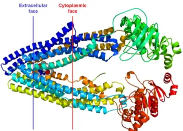
complexity of the individual transporters. P-glycoprotein (MDR1) is the archetypal human ABC

transporter, being the most medically relevant and well-studied. MDR1, Figure 1, is composed of

1280 amino acids (170 kDa) arranged as a single polypeptide.2 Although the corresponding gene

has been mapped, the crystal structure observed, and the amino acid sequence recorded,

determining the actual mechanism of poly-specific substrate selection is still a major challenge

for current bioinformatic techniques.4 Alternative methods in the field of cheminformatics

attempt to predict the interaction between substrate and protein without explicitly modelling the

transporter active site or the mechanism of selection and transport.6

(4)

In this study, we look at members of two major transporter families: the ATP-binding

cassette (ABC) superfamily and the solute carrier (SLC) group. Collectively, these groups

include the majority of identified proteins that contribute to drug resistance and susceptibility,

and understanding their biological differences may help explain differences in our ability to

predict their behavior.

ATP-Binding Cassette (ABC) Superfamily

The ABC superfamily of transporters is fundamental to life as it evolved on Earth;

members are believed to be present in every cell of every living organism.2 All ABC transporters

have two distinct substructures: a transmembrane domain (TMD, a portion of the protein that

tunnels through the cell membrane) and cytosolic nucleotide binding domain (NBD). ABC

proteins actively transport substrates through a series of conformational changes in the TMD that

are initiated by the binding and hydrolysis of adenosine triphosphate (ATP, the cell’s energy

molecule) to the NBD. Although the NBD is very similar in all ABC transporters, the TMD vary

widely, corresponding to variations in compatible substrates.

Solute Carrier (SLC) Group

In contrast to the evolutionary relatedness of ABC transporters, membership in the SLC

group is functional, encompassing all families of transmembrane solute transporters that are not

primary active transporters, ion channels, nor water channels. Accordingly, different SLC

subfamilies exhibit little structural similarity, also referred to has homology.3

Mechanisms of Transport

Membrane transporters form doorways through the cell membrane and operate by one of

three means:

 Passive transporters allow substrates to move naturally across the membrane from

regions of high electrochemical potential to regions of low potential. This flow down an

electrochemical gradient is energetically favorable and requires no additional energy.

 Primary active transporters are molecular motors that utilize an energy source, usually

ATP hydrolysis, to drive the movement of substrate.

 Secondary active transporters are molecular turbines that couple the movement of two

substrates simultaneously. The flow of one substrate down its gradient is used to power

(5)

ABC proteins undergo primary active transport while the SLC group includes both passive and

secondary active transporters.

Cheminformatics

Although the intersection of chemistry and informatics had been established by the

mid-1960s, the term “cheminformatics” was coined by F. K. Brown in 1998 as

“the mixing of those information resources to transform data into information and

information into knowledge for the intended purpose of making better decisions

faster in the area of drug lead identification and optimization.”7,8

One year later, at the August 1999 meeting of the American Chemical Society, G. Paris

broadened to the term to

“[encompass] the design, creation, organization, management, retrieval, analysis,

dissemination, visualization, and use of chemical information.”6

The new nomenclature was a symptom of the exploding interest in the field during the 1990s

brought about both by advances in synthetic techniques and increases in computational power. In

particular, the concurrent developments of combinatorial chemical synthesis and high-throughput

screening allowed chemists to collect data hundreds of thousands times faster than before, the

quantity of which conventional analytical techniques were simply unable to manage.8-10

In particular, cheminformatics seeks to reduce the time and capital costs of drug

discovery by better identifying potential candidates earlier in silico. Current drug discovery

techniques require an estimated fifteen-years and nearly two billion US dollars to bring a new

drug into the market.6,11 These costs are due to the immensity of the chemistry space as well as

the rigor of clinical trials. Computational techniques, however, are relatively fast and cheap and

can be employed to reduce the number of exploratory assays and studies necessary.12-14

Molecular Representation

Molecules are complex real-world objects. Even 3-dimensional topography models are

little more than illustrative simplifications of what are in reality infinite fields of electron density

associating infinitesimal points of mass and charge. Although many standards exist in practice,

the task of representing molecules in silico is neither trivial nor complete. A database of

molecules may be queried using the accepted common name or a unique registry number

assigned by the Chemical Abstracts Services (CAS). More informative representations reference

(6)

Figure 2. Standard cheminformatic representations for aspirin.6

Name Representation

Common Name Aspirin

Synonyms Acetylsalicylic acid, Ecotrin, Acenterine, Acylpyrin, Polopyryna, Acetophen, Acetosal, Aspergum

Empirical Formula C9H8O4

2D Structure

IUPAC Name 2-Acetoxybenzoic acid

CAS Registry Number 50-78-2

SMILES CC(=O)OC1=CC=CC=C1C(=O)O

InChl 1S/C9H8O4/c1-6(10)13-8-5-3-2-4-7(8)9(11)12/h2-5H,1H3,(H,11,12)

Connection Table (SDF)

Aspirin Comment Line

21 21 0 0 0 0 0 0 0 999 V2000

6.3301 -0.5600 0.0000 C 0 0 0 0 0 0 0 0 0 0 0 0 4.5981 -1.5600 0.0000 C 0 0 0 0 0 0 0 0 0 0 0 0 6.3301 -1.5600 0.0000 C 0 0 0 0 0 0 0 0 0 0 0 0 5.4641 -2.0600 0.0000 C 0 0 0 0 0 0 0 0 0 0 0 0 2.0000 -0.0600 0.0000 C 0 0 0 0 0 0 0 0 0 0 0 0 5.4641 -0.0600 0.0000 C 0 0 0 0 0 0 0 0 0 0 0 0 4.5981 -0.5600 0.0000 C 0 0 0 0 0 0 0 0 0 0 0 0 4.5981 1.4400 0.0000 O 0 0 0 0 0 0 0 0 0 0 0 0 2.8660 -1.5600 0.0000 O 0 0 0 0 0 0 0 0 0 0 0 0 6.3301 1.4400 0.0000 O 0 0 0 0 0 0 0 0 0 0 0 0 5.4641 0.9400 0.0000 C 0 0 0 0 0 0 0 0 0 0 0 0 2.8660 -0.5600 0.0000 C 0 0 0 0 0 0 0 0 0 0 0 0 3.7321 -0.0600 0.0000 O 0 0 0 0 0 0 0 0 0 0 0 0 6.3301 2.0600 0.0000 H 0 0 0 0 0 0 0 0 0 0 0 0 6.8671 -0.2500 0.0000 H 0 0 0 0 0 0 0 0 0 0 0 0 4.0611 -1.8700 0.0000 H 0 0 0 0 0 0 0 0 0 0 0 0 6.8671 -1.8700 0.0000 H 0 0 0 0 0 0 0 0 0 0 0 0 5.4641 -2.6800 0.0000 H 0 0 0 0 0 0 0 0 0 0 0 0 2.3100 0.4769 0.0000 H 0 0 0 0 0 0 0 0 0 0 0 0 1.4631 0.2500 0.0000 H 0 0 0 0 0 0 0 0 0 0 0 0 1.6900 -0.5969 0.0000 H 0 0 0 0 0 0 0 0 0 0 0 0 6 7 2 0 0 0 0

1 6 1 0 0 0 0 6 11 1 0 0 0 0 2 7 1 0 0 0 0 7 13 1 0 0 0 0 1 3 2 0 0 0 0 10 11 1 0 0 0 0 8 11 2 0 0 0 0 2 4 2 0 0 0 0 12 13 1 0 0 0 0 5 12 1 0 0 0 0 9 12 2 0 0 0 0 3 4 1 0 0 0 0 1 15 1 0 0 0 0 2 16 1 0 0 0 0 3 17 1 0 0 0 0 10 14 1 0 0 0 0 4 18 1 0 0 0 0 5 19 1 0 0 0 0 5 20 1 0 0 0 0 5 21 1 0 0 0 0 M END

(7)

(IUPAC) has defined explicit nomenclature standards, Simplified Molecular Input Line Entry

Specification (SMILES) defines rules for describing molecular structure using an ASCII string,

and the Structure Data Format (SDF) standards are the most commonly used graph-based

representation.6 Figure 2 illustrates several standard representations for aspirin.

The structure itself is usually not useful for analysis, so descriptors are generated from

the structural representation. Molecular descriptors are quantified features that describe the

salient aspects of the compound. Both open-source, e.g. CDK, and privately licensed, e.g.

Dragon, descriptor generators exist with their own individual sets of descriptors.6 There are two

primary classes of descriptors. Information-based descriptors encapsulate the structure of the

compound and include descriptors for the molecular weight, the number of rotatable bonds, and

Kier shape indices. Knowledge-based descriptors are calculated using known models and include

estimates of the polarity in different regions of the compound. The Dragon descriptor set is much

larger than CDK (2489 v. 202) and includes many more esoteric and hyper-specific descriptors,

e.g. the frequency of carbon-fluorine atom pairs exactly 10 bonds apart. In general, there is a

trade-off between interpretability and predictive usefulness.13

QSAR Modeling

Quantitative structure-activity relationship (QSAR) modelling may be described as the

use of computational, analytical, and statistical methods to accurately and reliably predict or

explain the properties or activities of chemical compounds provided only their structure.15

Chemical activity can be defined as any quantifiable and observable behavior. It may be a

classification (e.g. substrate or not), a regression (e.g. the rate of transport through a membrane),

or a categorization into an ordered set of classes (e.g. highly active, active, or inactive).16

As early as 1869, Alexander Crum Brown and Thomas Richard Fraser proposed that a

molecule’s activity can be defined as a mathematical function of its structure.6

Furthermore, the

structure-activity relationship hypothesis states that similar compounds possess similar

properties. Unfortunately, chemical similarity and diversity are oftentimes extremely difficult to

define, and different measures of similarity may be relevant when considering different

activities. QSAR modeling attempts to quantify a structure-activity relationship such that it may

(8)

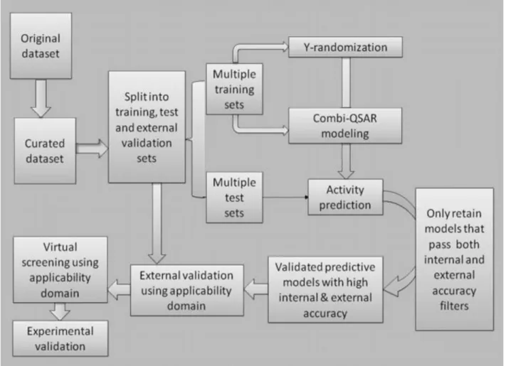
The predictive QSAR modeling workflow presented in Figure 3 has been adapted from

Tropsha 2010.15 The input to the QSAR workflow is always a dataset of compounds with

experimentally confirmed chemical activities. Thus the quality of a QSAR predictor is

fundamentally reliant on the quality of the experimental values and an accurate understanding

and representation of the chemical structures. It is critical to curate the chemical dataset to ensure

accurate structures and to remove any compounds that may not be informative to the model. If

chirality-sensitive descriptors are not employed, all pairs of mirror images will be represented as

duplicates; one must be removed, and any variance in their activities must be reconciled. In

addition, any compounds should be removed that cannot be handled by current techniques,

including organometallic complexes, inorganic compounds, salts, and mixtures.15

Any number of supervised learning techniques may then applied to the curated dataset to

construct the predictor, but the workflow remains the same.15 Firstly the dataset must be divided

(9)

into modeling and external sets. Usually many models are constructed from the modelling set,

and the best models, as identified by some internal evaluation, are consolidated to form the

predictor. To avoid overfitting, training is conducted using only the modelling set, and the

external set is used to validate the predictor.17 By considering the distribution of compounds, an

applicability domain (AD) is applied to each model as well as the overall predictor that defines

the subspace of the chemistry space for which the model has been validated.

Although there is a precedent for regulation based solely on predictive modelling,18 a

predictor should ideally be subject to laboratory validation. In silico high-throughput screening

of the predictor on compound databases will identify additional compounds with activities of

interest. The activities of some of these compounds should be determined experimentally to

further validate the predictor.15

Modeling Major Human Transporters

The human transportome consists of the subset of the proteome devoted to membrane

transporters. Recently, there have been several large-scale efforts to collect and organize the ever

increasing amount of transportome data available.19-23 Yet, until very recently, there has been

little effort to model this substrate data with the corresponding explicit molecular structures.1 In

this study, 56 datasets comprised of 10,407 activity values corresponding to the interaction

between 3,906 unique chemical compounds and 14 transporters were curated, characterized, and

modeled using multiple QSAR algorithms. The quality of the QSAR predictors was analyzed to

elucidate correlations with the chemical, biological, and numerical characters of the datasets.

Materials and Methods

Dataset Creation and Curation

Chemical-transporter interaction data were collected and curated by the Molecular

Modeling Lab in the Eshelman School of Pharmacy at the University of North Carolina at

Chapel Hill. Data were extracted from multiple publically available sources and consolidated

into 56 datasets.19-23 Equivalent records were compared and reconciled to form a single,

harmonious database. Classification datasets were constructed by combining reports of substrate

or inhibitory activity. Accordant reports were assigned values of 0 or 1, and ambiguous

chemicals were not included. Inhibitor classification is defined at a specified threshold

(10)

Michaelis-Menten constant of transportation (pKm, the relative concentration of substrate needed

to transport at a rate half of the maximum) or of the half maximal inhibitory concentration

(pIC50, the relative concentration of inhibitor needed to reduce the rate of transport by half). In

addition, datasets of pIC50 values are included for both general and specific hot ligands (the

substrate whose transport is being inhibited).

Chemical structures were standardized by the Molecular Modeling Lab using

PipelinePilot ver.6.15 (Accelrys) and the Standardizer module (ChemAxon).1 Organometallic

and poorly defined compounds were excluded from the database. In addition, polymers,

identified as extreme molecular weight outliers, were also excluded. Remaining compounds were

standardized and translated into their predominant and neutral form. The final curated database is

available on Chembench.26 The full, detailed process for data collection and curation has been

previously described by Sedykh et al.1

Dataset Characterization

The 56 datasets were preliminarily

characterized by their relevant transporter and

by the parameters of the activity reported (see

Tables 6 and 7 of the appendix). A summary

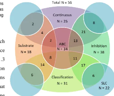
of the number of compounds in the datasets is available in Table 1. Twenty-five datasets

comprised of continuous values, and 31 contained binary assignments. Eighteen datasets

reported substrate activity, and 38 reported inhibitory activity (see Figure 5).

Transporters were also characterized by

the physiological role in the human body (see

Table 8 of the appendix and Figure 4).24 In all,

14 transporters from the ABC and SLC groups

are represented. Their membrane location,

direction of flow, subfamily, and archetypal

substrate are also reported and were included in

the statistical analysis.

Table 1. Summary of dataset cardinality.

Activity Type Max Min Mean St. Dev.

Classification

(N = 31) 1585 34 228.3 313.7

Continuous

(N = 25) 476 27 133.2 121.5

(11)

Descriptor Generation

Descriptors were generated for each

dataset using both the open-source

Chemistry Development Kit (CDK) ver.1.3

(202 descriptors) as well as Dragon

ver.1.4.4 (Talete) with explicit hydrogens

(2489 descriptors). Any descriptors that

generated an error for at least one

compound were dropped from the datasets. Descriptors were considered non-informative and

dropped from individual datasets if they correlated completely with another descriptor or if they

did not vary across compounds in that

dataset. Counts of retained descriptors for

individual classification and continuous

datasets are listed in Tables 6 and 7 of the

appendix and are summarized in Table 2.

Modelability Index Calculation

In a recent publication, Golbraikh et al. proposed the use of a MODelability Index

(MODI) to assess the goodness of a dataset for successful model building based on the frequency

of activity cliffs (regions in the descriptor space where chemical activity changes rapidly).25

They offer a definition for classification datasets computed from the number of dissimilar nearest

neighbors present for each class in the dataset:

(1)

where K is the number of classes, Nisame is the number of compounds belonging to the ith class

whose nearest neighbor belongs to the same class, and Nitotal is the total number of compounds in

the ith class. Nearest neighbors are determined as the neighbor with the least Euclidean distance Table 2. Summary of descriptors retained.

Descriptor Set Max Min Mean St. Dev.

CDK 162 127 151.6 8.4

Dragon 1420 835 1098.3 135.9

∑

(12)

from the compound in the entire descriptor space.25 Because descriptors are generated from the

chemical structure, the nearest neighbor will be the most structurally similar compound.

I offer a similar definition of MODI for continuous datasets for use and evaluation in this

study:

(2)

where N is the total number of compounds, z(ai) is the normalized activity of the ith compound,

and z( ) is the normalized activity of the neighbor nearest to the ith compound. Therefore MODI

is calculated as the average number of standard deviations in activity between nearest neighbors.

MODI values were computed for each transporter dataset using Python ver.2.7.6

including the packages NumPy and scikit-learn

ver.0.14. Descriptors were auto scaled before

calculating neighbor distances. MODI values

for individual classification and continuous

datasets are listed in Tables 6 and 7 of the

QSAR Modeling

Quantitative structure-activity relationship (QSAR) predictors were created using the

Carolina Cheminformatics Workbench (Chembench) developed by the Carolina Exploratory

Center for Cheminformatics Research (CECCR) and according to the workflow outlined in

Figure 3.26 Random forests (RFs) were generated using the randomForest package for R

ver.4.6-7, support vector machines (SVMs) were constructed using an grid-search built on libsvm, and

k-nearest neighbors (kNN) predictors were prepared using an internally developed KNN+ ver.2.82.

Meta-parameters for each predictor type were controlled across datasets.

Datasets were split into five equal folds for external cross-validation. Separate predictors

were generated and evaluated for each external fold and then consolidated into a single

consensus predictor. Internal test sets were selected by sphere exclusion for datasets with fewer

than 300 compounds and randomly otherwise. Predictors were created for each dataset using

either CDK or Dragon descriptor sets.

∑| ( ) ( )|

Table 3. Summary of dataset modelability indices.

Activity Type Max Min Mean St. Dev.

Classification

(N = 31) 0.98 0.39 0.75 0.11

Continuous

(13)

Continuous datasets were modeled using RF, SVM, and kNN. The kNN predictors were

trained using a genetic algorithm (GA-kNN) for datasets with greater than 150 compounds and

both GA-kNN and simulated annealing (SA-kNN) otherwise. Descriptors were normalized using

range scaling. Predictors were evaluated by the average coefficient of determination (R2) of the

five folds:

(3)

where yi is the observed activity of the ith compound, ŷi is the predicted activity of the ith

compound, and ȳ is the average activity of all compounds.15 Note that because the model

predictions are not a linear best fit, the sum of squared errors (SSE) may be greater than the total

sum of squares (SST) in the observed activities.

Therefore R2 values may be negative.17 Coefficients

of determination for individual regression

predictors, reported as the mean of five

cross-validation folds, are shown in Table 9 of the

As will be shown, modeling technique was not found to have a significant effect on

predictive power. Therefore, because of its rapid modeling time, classification datasets were

modeled using RF only. Four predictors were generated for each dataset corresponding to each

combination of range or auto scaled CDK or Dragon descriptors. Predictors were evaluated by

the overall correct classification rate (CCR) of the five folds:

(4)

where K is the number of classes (K = 2 for binary datasets), Ni,correct is the number of correctly

classified compounds in the ith class, and Ni,total is the total number of compounds in the ith class.

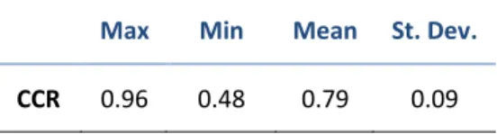
Previous studies have identified a CCR of 0.7 to

be the threshold for acceptable predictive

power.15,25 CCR, reported as the mean of five

cross-validation folds, are shown in Table 10 of

the appendix and are summarized in Table 5.

∑ ( ̂)

∑ ( ̅)

∑

Table 4. Summary of coefficients of determination for regression predictors.

Max Min Mean St. Dev.

R2 0.82 -0.20 0.37 0.22

Table 5. Summary of correct classification rates for classification predictors.

Max Min Mean St. Dev.

(14)

Model Fortification

Predictors were subjected to several additional thresholds throughout the modeling

process to maximize predictive power. Datasets with fewer than 30 compounds were not

modeled (N = 2). Individual models were required to present a squared leave-one-out

cross-validation correlation coefficient (Q2) of at least 0.6 to be accepted.

In addition, stochastic models were identified using y-randomization. This process

randomly redistributes activities to the compounds in the modeling set, constructs a predictor,

and calculates a CCR or R2 using a fraction of the modeling set as an evaluation set. Five

y-randomized predictors are constructed in this way such that a one-tailed t-test could be conducted

to determine the probability of obtaining the CCR or R2 of the true-activity predictor with

randomized values. If the p-value was greater than 0.05, the models built using the real data were

deemed unreliable and rejected.

An applicability domain (AD) of 0.5 standard deviations was also applied to each model

of kNN predictors. The standard deviation in Euclidean distance in the descriptor space between

each compound and its k nearest neighbors was calculated. Models were ignored during

prediction and evaluation if the new compound did not have at least k neighbors within 0.5

standard deviations.

In all, 274 predictors passed all cut-offs. The five datasets with fewer than 50 compounds

(N = 5) failed to produce any kNN models that passed all cut-offs. In addition, two datasets with

51 compounds failed to generate adequate models for a single kNN predictor each.

Statistical Analysis

Dataset characterization data and predictor quality data were prepared for analysis using

Excel ver.14.0 (Microsoft). Statistical analyses were conducted using Stata ver.13.0 (StataCorp).

Results and Discussion

A series of linear regression analyses were conducted to reveal correlations between the

biological, chemical, and numerical characteristics of the datasets and the modelability as

expressed by the coefficient of determination (R2) or correct classification rate (CCR) of the

predictor. These results may be used to improve future QSAR studies as well as to identify

(15)

Quantifying Predictive Power

The coefficient of determination (R2) calculated for continuous predictors is a measure of

the sum of squares of the external validation. Unfortunately, this value does not lend itself well

to linear regression. In addition, some values of R2 were found to be negative. Therefore a

transformed root of squares (R1) was used for analysis:

(5)

where R2 is the coefficient of determination.

Although it may be tempting to make conclusions about the relative success of regression

and classification QSAR predictors, it should be emphasized that R1 (equations (3) and (5)) and

CCR (equation (4)) are distinct evaluation measures that are not comparable. Both R1 and CCR

asymptotically approach 1.0 as external prediction improves. However, while R1 ranges to

negative infinity, CCR has a minimal value of zero. A random assignment of regression

predictions from the observed distribution will result in an R of 0.0, but a random classification

will result in a CCR of the inverse of the number of classes (CCR = 0.5 for binary data sets).

Therefore all analyses were conducted separately on either regression or classification predictors.

Numerical Characteristics

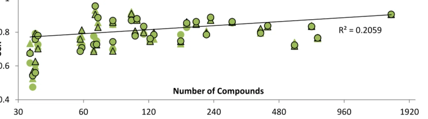
Not surprisingly, the size of a dataset was found to have a significant positive correlation

(p < 0.001) with predictive power for both regression and classification datasets. Furthermore,

this correlation is best realized when the dataset size is represented by the logarithm of the

cardinality. Figures 6 and 7 plot the R1 values for each regression predictor and CCRs for each

classification predictor, respectively, against the size of the original dataset.

√

Figure 6. Correlations between the logarithm of the number of compounds and the R1 of regression predictors. CDK (circles) and Dragon (triangles) descriptors are denoted by shape. RF (green), SVM (blue) and kNN (orange) are denoted by color.

R² = 0.276

-0.2 0 0.2 0.4 0.6

35 70 140 280

R1

(16)

In addition, QSAR modeling technique, descriptor type, and descriptor scaling are

denoted for each datum in Figures 6 and 7. None of these characteristics, nor the number of

descriptors, had a statistically significant effect on predictive power for either continuous or

classification datasets when controlling for the size of the dataset.

Modelability Indices

Classification MODI

The definition of a Modelability Index (MODI) offered by Golbraikh et al.25 and

presented again here as equation (1) was found to be a strong indicator of the predictive power of

RF classification transporter datasets. A significant correlation (R2 = 0.72) was found between

MODI and a predictor’s external CCR. Figure 8 is a plot of each predictor’s CCR against the

MODI of its original dataset. Using the threshold for modelability also offered by Golbraikh et

al. (CCR > 0.7), MODI can be used to reliably estimate whether a dataset may yield an

acceptable predictor. Nearly all (N = 107 of 112) predictors built from datasets with MODI

above 0.64 resulted in a CCR greater than 0.7.

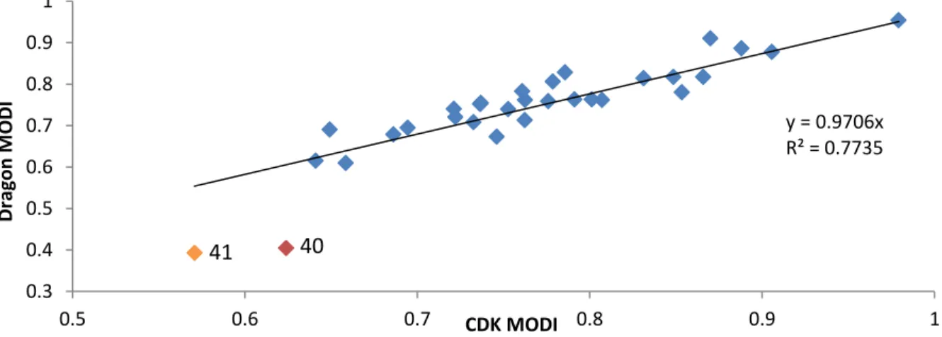
In addition, descriptor type, and by extension the number of descriptors, was not found to

affect the MODI of a dataset. Figure 8 is a plot of the MODI calculated using Dragon descriptors

versus the MODI calculated using CDK descriptors for each classification dataset. A significant

correlation (R2 = 0.77) was determined for a linear regression through the origin. Note that only

two datasets deviate from this trend: datasets 41 and 40 located in the lower left of Figure 9. The

discrepancy in MODI implies that the compounds in these datasets are represented differently in

some significant way in the different descriptor spaces. These datasets are both concerned with R² = 0.2059

0.4 0.6 0.8 1

30 60 120 240 480 960 1920

CCR

Number of Compounds

Figure 7. Correlations between the logarithm of the number of compounds and the CCR of

(17)

the inhibition of MRP3 at different thresholds. Cross referencing Figure 8 reveals that the MODI

calculated using Dragon descriptors better predicted the CCR of the resultant predictors.

Therefore it may be inferred that CDK does not include some key descriptors relevant to MRP3

inhibition. However, any major conclusions from these datasets should be avoided because they

contain relatively few compounds (N = 36 and 35).

In addition, this set of datasets is biased toward modelable datasets. Additional predictors

with CCR between 0.5 and 0.7 would need to be studied to verify the correlation in the

unmodelable quadrant of Figure 8.

y = 0.7238x + 0.2416 R² = 0.7219

0.4 0.5 0.6 0.7 0.8 0.9 1

0.3 0.4 0.5 0.6 0.7 0.8 0.9 1

CCR

MODI Dragon

CDK

Modelable

Unmodelable

Figure 8. Correlation between the CCR of classification predictors and the MODI of their original datasets. The threshold for modelability is marked at CCR = 0.7 and correspondingly at MODI = 0.63. Datasets 40 (red) and 41(orange) are identified from Figure 9.

y = 0.9706x R² = 0.7735

0.3 0.4 0.5 0.6 0.7 0.8 0.9 1

0.5 0.6 0.7 0.8 0.9 1

D

rag

o

n

M

OD

I

CDK MODI

41 40

(18)

Continuous MODI

A novel definition for the MODI of continuous datasets was introduced in equation (2). A

significant correlation (R2 = 0.59) was found between values calculated using this definition of MODI and a regression predictor’s R1

value. Figure 10 illustrates this relationship with

descriptor type and modeling technique identified. Using a coefficient of determination of R2 >

0.5 as the threshold for modelability15 corresponds to a root of squares of roughly R1 > 0.3.

Therefore I propose a heuristic threshold of MODI > 0.35 to estimate the modelability of

continuous datasets. This cutoff deviates from the regression line to increase sensitivity without

sacrificing precision in this set.

Biological Characteristics

The membrane transporters were divided into homologous groups for additional analysis.

Because all ABC transporters are related, this process grouped ABC together and SLC

transporters into subfamilies. A statistically significant correlation was determined between this

grouping and the predictive power of classification datasets. In particular, predictors concerning

SLC transporters reported CCRs 0.089 greater (p < 0.001) than ABC predictors, on average. This

correlation persists when dataset size and MODI are included in the regression. Figure 11

illustrates the way that ABC predictors evaluated more poorly, even when the original datasets

computed similar MODI. This indicates that there are additional factors affecting modelability y = 0.8386x - 0.0398

R² = 0.5909

-0.1 0 0.1 0.2 0.3 0.4 0.5 0.6

0 0.1 0.2 0.3 0.4 0.5 0.6

R1

MODI Unmodelable

Modelable

(19)

besides those captured by MODI. This trend may result from the interaction with ATP as the

energy source or it may indicate that ABC transporters are reliant on the selectivity of multiple

external binding proteins.

Additional features characterizing the membrane transporter and activity measure were

analyzed as well. The location of the transporter in vivo, whether in the basal or apical

membranes, was not found to be significant for predictive power. Whether the dataset included

inhibitor or substrate activity data, however, was significant for both classification and regression

predictors when controlling for dataset size. Curiously, classification inhibitor datasets predicted

CCR 0.034 less (p = 0.022) than their substrate counterparts on average, but continuous inhibitor

datasets evaluated with R1 0.080 greater (p = 0.007) on average. This discrepancy is not quickly

explained, and additional research is needed to determine which, if either, correlation is accurate.

Conclusions

Membrane transport proteins are directly responsible for the movement of chemicals into

and out of each cell, so predicting their interaction with potential drug candidates is an important

challenge for drug discovery.1 Quantitative structure-activity relationship (QSAR) modeling, as

part of the greater field of cheminformatics, attempts to predict the activity of new compounds

by comparing their structures with the structures of compounds with known interactions. This

technique was applied to 56 datasets concerning 14 major human transporters. A modelability

index (MODI) for chemical datasets of continuous activities was developed to mimic an existing 0.4

0.5 0.6 0.7 0.8 0.9 1

0.3 0.4 0.5 0.6 0.7 0.8 0.9 1

CCR

MODI

(20)

MODI for classification datasets as a heuristic device for estimating predictive power. Dataset

cardinality and MODI were found to have significant effects on predictive power, but modeling

technique and descriptor type were not. In addition, transporter homology group was found to

have a significant effect such that ABC datasets modeled more poorly, on average. This suggests

that the mechanism of substrate selection of ABC proteins is more complex than that of SLC

proteins. True validation of QSAR predictors requires laboratory experimentation, which was not

available for this study.15 Therefore additional research is needed to confirm the predictive

powers of each dataset and verify the correlations observed.

Acknowledgements

I would like to express my deepest thanks to Professor Pozefsky for her guidance and

support throughout the course of this study in all its stages. I would like to thank also Ian Kim for

his help with the Chembench system, the members of the Molecular Modeling Lab for providing

the datasets, funding, and initiative to make this project possible, each previous Chembench

developer, and all of the other students, faculty, and staff of the departments of Computer

Science and Chemistry.

References

1. Sedykh, A.; Fourches, D.; Duan, J.; Hucke, O.; Garneau, M.; Zhu, H.; Bonneau, P.;

Tropsha, A. Human Intestinal Transporter Database: QSAR Modeling and Virtual

Profiling of Drug Uptake, Efflux, and Interactions. Pharm. Res.2013, 30, 996-1007.

2. Jones, P. M.; George, A. M. The ABC transporter structure and mechanism: perspectives

on recent research. Cell Mol. Life Sci.2004,61(6), 682–99.

3. Hediger, M. A.; Romero, M. F.; Peng, J. B.; Rolfs, A.; Takanaga, H.; Bruford, E. A. The

ABCs of solute carriers: physiological, pathological and therapeutic implications of

human membrane transport proteins: Introduction. Pflugers Arch.2004, 447(5), 465–8.

4. Aller, S. G; Yu, J.; Ward, A.; Weng, Y.; Chittaboina, S.; Zhuo, R.; Harrell, P. M.; Trinh,

Y. T.; Zhang, Q.; Urbatsch, I. L.; et al. Structure of P-Glycoprotein Reveals a Molecular

Basis for Poly-Specific Drug Binding. Science2009, 323(5922), 1718-1722.

5. Wikimedia Commons: http://en.wikipedia.org/wiki/File:MDR3_3g5u.png

6. Brown, N. Chemoinformatics--an introduction for computer scientists. ACM Comput.

(21)

7. Brown, F. K. Chapter 35. Cheminformatics: What is it and How does it Impact Drug

Discovery. Ann. Rep. Med. Chem.1998, 33.

8. Russo, E. Chemistry plans a structural overhaul. Nature Jobs2002, 419, 4–7.

9. Willett, P. A Bibliometric analysis of chemoinformatics. Aslib Proc.2008, 60, 4-17.

10.Hann, M.; Green, R. Chemoinformatics - a new name for an old problem? Chem. Biol.

1999, 3, 379-383.

11.Chen, W. L. Chemoinformatics: past, present and future. J. Chem. Inf. Mod. 2006, 46,

2230-2255.

12.Gasteiger, J. Chemoinformatics: a new field with a long tradition. Anal. Bioanal. Chem.

2006, 384, 57-64.

13.Maldonado, A. G.; et al. Molecular similarity and diversity in chemoinformatics: from

theory to applications. Mol. Div.2006, 10, 39-79.

14.Willett, P. From chemical documentation to chemoinformatics: fifty years of chemical

information science. J. Inf. Sci.2008, 34, 477-499.

15.Tropsha, A. Best Practices for QSAR model Development, Validation, and Exploitation.

Mol. Inf.2010, 29, 476-488.

16.Nantasenamat, C.; Isarankura-Na-Ayudhya, C.; Naenna, T.; Prachayasittikul, V. A

Practical Overview of Quantitative Structure-Activity Relationship. EXCLI J. 2009, 8,

74-88.

17.Esposito, E. X.; Hopfinger, A. J.; Madura, J. D.; Methods for Applying the Quantitative

Structure-Activity Relationship Paradigm. In Chemoinformatics: Concepts, Methods, and

Tools for Drug Discovery; Bajorath, J., Ed.; Totowa: New Jersey, 2004; pp 131-213.

18.OECD Principles for the Validation of (Q)SARs. European Commission Joint Research

Centre. Institute for Health and Consumer Protection, 30 June 2011. Web. 19 Apr. 2014.

19.Giacomini, K. M.; Huang, S. M.; Tweedie, D. J.; Benet, L. Z.; Brouwer, K. L. R.; Chu,

X.; et al. Membrane transporters in drug development. Nat. Rev. Drug Discov. 2010, 9,

215-36.

20.Saier Jr., M. H.; Yen, M. R.; Noto, K.; Tamang, D. G.; Elkan, C. The transporter

classification database: recent advances. Nucleic Acids. Res.2009, 37, D274-8.

21.Yee, S. W.; Chen, L.; Giacomini, K. M. Pharmacogenomics of membrane transporters:

(22)

22.Ozawa, N.; Shimizu, T.; Morita, R.; Yokono, Y.; Ochiai, T.; Munesada, K.; et al.

Transporter database, TP-Search: a web-accessible comprehensive database for research

in pharmacokinetics of drugs. Pharm. Res.2004, 21, 2133-4.

23.Ren, Q.; Chen, K.; Paulsen, I. T. TransportDB: a comprehensive database resource for

cytoplasmic membrane transport systems and outer membrane channels. Nucleic Acids

Res.2007, 35, D274-9.

24.Gene Database. National Center for Biotechnology Information.

<http://www.ncbi.nlm.nih.gov/gene/>

25.Golbraikh, A.; Muratov, E.; Fourches, D.; Tropsha, A. Data Set Modelability by QSAR.

J. Chem. Inf. Model. 2014, 54, 1-4.

(23)

Appendix

Table 6. Characterization data for continuous datasets.

Transporter Activity Hot Ligand a

Number of Compounds

Number of Descriptors b Modelability Index c

CDK Dragon CDK Dragon

Substrate Datasets

ASBT pKm 51 127 878 0.234 0.147

MDR1 pKm 63 152 1,015 0.226 0.059

MRP2 pKm 27 148 944 0.081 0.000

PEPT1 pKm 72 133 845 0.411 0.329

Inhibition Datasets

ASBT pIC50 Taurocholate 341 159 1,243 0.565 0.576

BCRP pIC50 Any 119 155 1,096 0.420 0.394

BCRP pIC50 Mitoxantrone 46 138 902 0.389 0.452

BSEP pIC50 Taurocholate 295 160 1,215 0.175 0.166

MCT1 pIC50 Any 46 142 955 0.114 0.279

MDR1 pIC50 Any 476 159 1,229 0.378 0.383

MDR1 pIC50 Calcein AM 116 154 1,119 0.374 0.306

MDR1 pIC50 Daunorubicin 302 152 1,164 0.364 0.413

MDR1 pIC50 Vinblastine 48 140 942 0.148 0.167

MRP1 pIC50 Any 196 151 1,056 0.474 0.391

MRP1 pIC50 Calcein AM 54 140 943 0.426 0.236

MRP1 pIC50 Daunorubicin 108 139 951 0.325 0.341

MRP2 pIC50 Any 103 154 1,138 0.344 0.313

MRP2 pIC50 DNP-SG 46 145 971 0.466 0.532

MRP4 pIC50 Any 40 143 987 0.228 0.240

NTCP pIC50 Taurocholate 75 155 1,099 0.162 0.177

OATP2B1 pIC50 Any 27 146 1,010 0.412 0.202

OCT1 pIC50 Any 87 149 981 0.068 0.207

OCT1 pIC50 Tetraethylammonium 51 148 949 0.196 0.286

PEPT1 pIC50 Any 272 155 1,149 0.412 0.326

PEPT1 pIC50 Glycylsarcosine 269 154 1,147 0.408 0.323

a

(24)

Table 7. Characterization data for classification datasets.

Transporter Activity a

Threshold (μM)

Number of Compounds

Number of Descriptors b Modelability Index c

CDK Dragon CDK Dragon

Substrate Datasets

ASBT Substrate 106 144 1,064 0.906 0.877 BCRP Substrate 169 160 1,227 0.722 0.720 BSEP Substrate 34 140 924 0.733 0.708 MCT1 Substrate 36 138 835 0.694 0.694 MDR1 Substrate 567 162 1,347 0.686 0.679 MRP1 Substrate 180 160 1,206 0.849 0.817 MRP2 Substrate 222 160 1,192 0.736 0.752 MRP3 Substrate 100 158 1,075 0.870 0.910 MRP4 Substrate 122 159 1,187 0.762 0.713 MRP5 Substrate 58 152 1,092 0.776 0.759 NTCP Substrate 70 153 1,065 0.786 0.829 OATP2B1 Substrate 59 153 1,046 0.649 0.691 OCT1 Substrate 82 154 1,124 0.866 0.817 PEPT1 Substrate 292 158 1,176 0.807 0.762

Inhibition Datasets

ASBT Inhibitor 10 232 159 1,217 0.853 0.780 BCRP Inhibitor 10 395 162 1,266 0.762 0.762 BSEP Inhibitor 10 679 162 1,387 0.753 0.740 BSEP Inhibitor 100 725 162 1,393 0.791 0.763 MCT1 Inhibitor 10 68 147 1,028 0.979 0.954 MDR1 Inhibitor 10 1,585 162 1,420 0.888 0.886 MRP1 Inhibitor 10 426 158 1,242 0.831 0.814 MRP2 Inhibitor 10 104 153 1,127 0.721 0.740 MRP3 Inhibitor 10 36 154 1,048 0.624 0.405 MRP3 Inhibitor 50 35 154 1,061 0.571 0.393 MRP4 Inhibitor 10 67 148 1,069 0.641 0.615 MRP4 Inhibitor 50 69 148 1,074 0.761 0.783 MRP5 Inhibitor 50 37 144 1,030 0.801 0.763 NTCP Inhibitor 10 127 158 1,171 0.746 0.673 OATP2B1 Inhibitor 100 114 159 1,122 0.737 0.754 OCT1 Inhibitor 100 199 159 1,162 0.779 0.806 PEPT1 Inhibitor 100 82 141 956 0.659 0.610

a

(25)

Table 8. Characterization data for each transporter represented in the database.

Transporter Gene Membrane Direction Superfamily Subfamily Substrate

MDR1 ABCB1 Apical Efflux ABC MDR Xenobiotics

BSEP ABCB11 Apical Efflux ABC MDR Bile Acids

MRP1 ABCC1 Basal Efflux ABC MRP Organic Anions

MRP2 ABCC2 Apical Efflux ABC MRP Bile Acids

MRP3 ABCC3 Basal Efflux ABC MRP Organic Anions

MRP4 ABCC4 Basal Efflux ABC MRP Cyclic Nucleotides

MRP5 ABCC5 Basal Efflux ABC MRP Cyclic Nucleotides

BCRP ABCG2 Apical Efflux ABC White Xenobiotics

NTCP SLC10A1 Basal Influx SLC SLC10 Bile Acids

ASBT SLC10A2 Apical Influx SLC SLC10 Bile Acids

PEPT1 SLC15A1 Apical Influx SLC SLC15 Oligopeptides

MCT1 SLC16A1 Apical Influx SLC SLC16 Monocarboxylates

OCT1 SLC22A1 Basal Influx SLC SLC22 Organic Cations

(26)

Table 9. External validation results (R2, %) for transporter regression predictors.

Trans-porter

Hot

Ligand a

CDK Descriptors Dragon Descriptors

RF SVM GA-kNN b SA-kNN b,c RF SVM GA-kNN b SA-kNN b,c

Substrate Predictors

ASBT 27 ± 16 15 ± 39 failed 32 ± 36 27 ± 20 -2 ± 20 14 ± 39 3 ± 29 MDR1 -5 ± 17 12 ± 34 -9 ± 58 22 ± 44 2 ± 30 13 ± 13 6 ± 51 25 ± 28 PEPT1 41 ± 16 23 ± 29 23 ± 24 30 ± 26 23 ± 18 38 ± 17 39 ± 24 45 ± 19

Inhibition Predictors

ASBT Tauro. 82 ± 3 80 ± 2 75 ± 9 77 ± 7 BCRP Any 53 ± 14 55 ± 8 59 ± 13 51 ± 15 BCRP Mitox. 55 ± 25 31 ± 28 failed failed BSEP Tauro. 27 ± 10 7 ± 10 failed --- MCT1 Any 21 ± 23 23 ± 35 failed failed MDR1 Any 55 ± 9 51 ± 10 52 ± 6 --- MDR1 Calc.-AM 57 ± 15 50 ± 29 55 ± 6 57 ± 6 MDR1 Dauno. 57 ± 10 54 ± 11 59 ± 7 --- MDR1 Vinbl. 8 ± 55 -12 ± 55 failed failed MRP1 Any 62 ± 7 64 ± 6 61 ± 9 --- MRP1 Calc.-AM 44 ± 24 47 ± 36 27 ± 39 60 ± 20 MRP1 Dauno. 53 ± 6 54 ± 15 46 ± 11 54 ± 10 MRP2 Any 29 ± 25 -8 ± 76 42 ± 19 40 ± 11 MRP2 DNP-SG 50 ± 23 41 ± 35 failed failed MRP4 Any 11 ± 27 8 ± 17 failed failed NTCP Tauro. 27 ± 15 -9 ± 14 9 ± 19 9 ± 11 OCT1 Any 34 ± 28 8 ± 41 29 ± 28 34 ± 24 OCT1 N(Et)4 41 ± 31 34 ± 8 19 ± 45 26 ± 39 PEPT1 Any 46 ± 8 47 ± 16 45 ± 1 --- PEPT1 Glycyl. 48 ± 8 27 ± 25 29 ± 21 --- 79 ± 4 79 ± 3 73 ± 5 81 ± 4 44 ± 7 56 ± 11 60 ± 7 58 ± 8 36 ± 43 54 ± 18 failed failed 30 ± 18 37 ± 12 5 ± 18 --- 44 ± 16 33 ± 13 failed failed 55 ± 7 57 ± 8 52 ± 7 --- 60 ± 4 59 ± 10 53 ± 9 56 ± 10 61 ± 8 60 ± 9 60 ± 6 --- 12 ± 34 37 ± 27 failed failed 63 ± 5 61 ± 7 59 ± 11 --- 31 ± 21 45 ± 9 46 ± 29 48 ± 8 49 ± 14 54 ± 5 38 ± 22 50 ± 8 19 ± 33 55 ± 14 34 ± 8 41 ± 7 45 ± 19 68 ± 30 failed failed 18 ± 44 12 ± 36 failed failed 21 ± 14 -20 ± 62 10 ± 14 10 ± 23 40 ± 20 16 ± 25 33 ± 33 34 ± 30 27 ± 36 59 ± 15 failed 36 ± 26 40 ± 18 39 ± 12 33 ± 19 --- 38 ± 13 28 ± 17 33 ± 15 ---

(27)

Table 10. External validation results (CCR, %) for classification transporter predictors.

Transporter

Threshold a (μM)

CDK Descriptors Dragon Descriptors

Range Auto Range Auto

Substrate Predictors

ASBT 87 ± 7 88 ± 7 88 ± 9 87 ± 9

BCRP 79 ± 3 75 ± 3 73 ± 4 75 ± 3

BSEP 62 ± 19 68 ± 22 73 ± 18 68 ± 16

MCT1 79 ± 13 76 ± 12 76 ± 12 79 ± 8

MDR1 72 ± 3 72 ± 3 74 ± 5 72 ± 5