Sharif University of Technology
Scientia IranicaTransactions A: Civil Engineering www.scientiairanica.com
Reliability analysis of foundation settlement by
stochastic response surface and random nite-element
method
A. Johari
and A. Sabzi
Department of Civil and Environmental Engineering, Shiraz University of Technology, Shiraz, Iran. Received 21 October 2015; received in revised form 20 April 2016; accepted 22 August 2016
KEYWORDS Foundation settlement; Spatial variability; Random elds; Stochastic response surface method; Random nite-element method; Karhunen-Loeve expansion.
Abstract. This paper presents a reliability-based analysis of strip-footing settlement by Stochastic Finite-Element Method (SFEM). The Stochastic Response Surface Method (SRSM) and Random Finite-Element Method (RFEM) are used as two formulations of SFEM. The elastic properties of soil are considered as spatial random variables and modeled as cross correlated log-normal random elds. Random eld discretization is done by Karhunen-Loeve (K-L) expansion. Two programs were coded by MATLAB so as to take full advantages of its matrix operations, and in an illustrative example, it was shown that the results of SRSM are close to RFEM; however, the consumed time in RFEM is at most 50 times longer than that in SRSM. Using the faster method, SRSM, it is concluded that considering the spatial variability of soil parameters in stochastic analysis is necessary. © 2017 Sharif University of Technology. All rights reserved.
1. Introduction
The soil properties are inherently uncertain parame-ters. These properties are spatial variables and vary from one point in space to another. This leads to the necessity of representing the soil parameters as char-acterized random elds. In conventional approaches to foundation settlement determination, average values of soil parameters are considered and parameters' uncer-tainties are taken into account by applying a global Factor of Safety (FS). Probabilistic analysis provides a tool to consider the uncertain parameters in analysis.
There have been some scientic eorts directed at applying reliability analysis to the civil engineering tasks [1,2].
Many methods have been developed for
prob-*. Corresponding author.
E-mail address: [email protected] (A. Johari) doi: 10.24200/sci.2017.4169
abilistic/stochastic analysis of foundations on soils. Some of these are Monte Carlo Simulation (MCS), First-Order Reliability Method (FORM), Second-Order Reliability Method (SORM), Perturbation the-ory, SRSM, etc. [3]. For example, Shyamala and Dodagoudar [4] used Point Estimation Method (PEM) and First-Order Second Moment (FOSM) along with the non-linear nite-element analysis to evaluate the re-liability index in rere-liability analysis of shallow founda-tion settlements. The menfounda-tioned methods are clubbed with nite-element method to stochastic analysis of foundation settlement giving rise to methods like SFEM and RFEM. Among above methods, the RFEM and SRSM are two powerful methods to propagate in-put parameters uncertainties in nite-element models. In RFEM, the random elds are combined with the nite-element method through MCS. The RFEM has been widely used in geotechnical problems [5-9]. For example, Fenton and Griths [6] presented relia-bility analysis of foundation settlement by modeling the soil as spatially random media. Prediction of
settlement below the foundation was obtained using the nite-element method. Griths and Fenton [7] compared the reliability results of foundation settle-ment, obtained by stochastic nite-element method based on rst-order second-moment approximations, with the result of random nite-element method based on generation of random elds combined with Monte Carlo simulations. Pieczynska-Kozlowska et al. [10] studied the inuence of embedment, soil self-weight, and anisotropy of random eld on bearing capacity of foundation using RFEM.
In SRSM, the complex numerical model is re-placed by an analytical one, which is less time-consuming compared with original numerical model (deterministic model). The SRSM can be adopted in both linear and nonlinear problems, and all sta-tistical moments of outputs can be computed using this method. The SRSM has been used in many problems [11-19]. Among important contributions are the research studies of Huang et al. [14], Li et al. [17], Li and Zhang [18], and Jiang et al. [16]. Huang et al. [14] presented an extended stochastic response-surface method for problems in which physical properties exhibit spatial random variation by using collocation points as samples for constructing the output response surface. Li et al. [17] proposed a stochastic response surface method for reliability anal-ysis involving correlated non-normal random variables. They formulated the closed-form expressions for fourth to sixth order Hermit polynomial chaos expansions involving any number of random variables. Li and Zhang [18] explored a method for uncertainty analysis of ow in random porous media by combining the KL expansion and the SRSM based on Probabilistic Collocation Method (PCM). Jiang et al. [16] proposed a non-intrusive stochastic nite-element method for slope reliability analysis considering spatial variability of shear strength parameters. They adopted the K-L expansion to discretize the 2-Dimentional (2-D) cross-correlated non-Gaussian random elds of spatially variable shear strength parameters.
The objective of this paper is to analyze the reli-ability of strip foundation settlement by SRSM, which requires low computational time and low memory requirements; then, a comparison will be made between the obtained results with those of RFEM. In reliability analysis by SRSM, the model outputs are represented as functions of standard normal variables by polyno-mial chaos expansion. The unknown coecients in the polynomial chaos expansion are determined using a probabilistic collocation method. For modeling the soil behavior, elastic-perfectly plastic Mohr-Coulomb yield criterion, which is common in geotechnical problems, is used. In elastic-perfectly plastic models, hardening or softening which shows a more real behavior of soil cannot be considered. Each spatially random variable
is modeled as cross correlated log-normal 2-D random eld. The log-normal distribution is selected by the fact that the values of soil parameters are strictly positive. The well-known K-L expansion is used for random led discretization. Furthermore, an example is presented to compare the predictions of the SRSM and RFEM on the reliability analysis of settlement strip foundation.
2. Shallow foundation settlement
Foundation settlement will occur when a foundation is subjected to load. Excessive settlements may lead to serviceability problems and the desired use of the structure may be impaired. The foundation settlement depends on soil type and the water table level. It consists of three components: immediate settlement, consolidation settlement, and secondary compression. Classical formulations are available for computing these components of settlements. Numerical methods, such as nite-element and nite-dierence methods, can be used to calculate foundation settlement. These methods provide the advantage of idealizing the ma-terial behavior of soil, which is non-linear with plastic deformations and path dependent, in a more rational manner. In this study, the nite-element method is used to determine the foundation settlement.
3. Random eld modeling of soil properties The soil properties are spatial variables and vary from one point in space to another. The spatial variability of soil properties can be due to variations in min-eralogical composition, conditions during deposition, stress history, and physical and mechanical decompo-sition processes [20,21]. This leads to the necessity of representing the soil parameters as characterized random elds. Spatial variability of soil properties can be modeled using theory of random elds [22]. In the theory of random elds, at any location within a soil layer, the soil parameter is an uncertain quantity or a random variable which is characterized by a probability distribution and is correlated with the random variables at adjacent locations [20].
The values of a soil parameter are correlated at dierent points of a eld. The spatial correlation of soil parameter is considered by autocorrelation function. The autocorrelation function of a given soil parameter can be estimated from the measured data of the parameter at dierent locations [23]. In this study, for all uncertain parameters, a squared exponential 2-D autocorrelation function is assumed with dierent autocorrelation distances in the horizontal and vertical directions as follows:
(x; x0) = exp jx x0j
lx
jy y0j
ly
where x and x0 are spatial coordinates, and l
x and ly
are autocorrelation lengths in horizontal and vertical directions, respectively. Small values of the autocor-relation lengths imply a rapid uctuation about the soil parameter. However, high values imply a slowly varying soil parameter. In the case of 2-D problems, it is assumed that out-of-plane autocorrelation length is innite. If spatial variability of out-of-plane un-certain parameter be considered, 3-dimensional nite-element analysis should be done to consider its ef-fects.
3.1. Discretization of random elds
The numerical methods, such as nite-element formu-lation, have discrete nature; therefore, a continuous-parameter random eld must also be discretized into random variables. This process is commonly known as a discretization of a random eld. There are several methods to discretize a random eld in the litera-ture [24]. More ecient approaches for discretization of random elds are series expansion methods.
The series expansion methods can be done by three methods [24]: the K-L expansion, Orthogonal Series Expansion (OSE), and the Expansion Optimal Linear Estimation (EOLE) methods. K-L expansion is able to use a few terms to capture the characteristic of the strongly correlated random elds [25]. In this study, the K-L expansion is used. This method is introduced briey in the next subsection.
3.1.1. Karhunen-Loeve expansion
The K-L expansion of a random eld is based on the spectral decomposition of its autocorrelation function (x; x0). The set of deterministic functions, over which
any realization of eld H(x; ) is expanded, is dened by eigenvalue problem:
Z
(x; x 0)'
i(x0)dx0 = i'i(x); (2)
where x and x0denote the coordinates of two points in
space; 'i(x) and i are eigenfunctions and eigenvalues
of one-dimensional autocorrelation function (x; x0),
respectively. The eigenmodes of the separable multi-dimensional autocorrelation function are calculated through multiplying them by the eigenmodes obtained from Eq. (2). This integral can be solved analytically or numerically [26,27]. In this study, the closed form presented by Zhang and Lu [28] is used. The series expansion of a random eld H(x; ) is expressed as follows:
H(x; ) = +X1
i=1
pi'i(x)i(); x 2 ; (3)
where is mean and is standard deviation of the eld; i() is a vector of uncorrelated standard normal
variables, and indicates the random nature of the H(x; ). Practically, the series is approximated by a nite number of terms:
H(x; ) = +
M
X
i=1
pi'i(x)i(); x 2 : (4)
The value of M strongly depends on the desired accuracy and on the autocorrelation function of the random eld [29]. Small values of the autocorrelation lengths will lead to a signicant increase in the number of the K-L terms (M).
3.1.2. Cross correlated lognormal random elds Typically, more than one random soil parameter, such as Young's modulus, Poisson's ratio, the cohesion, and the friction angle, is involved in geotechnical problems. Among these, some soil parameters show the degree of dependency on each other. In other words, these parameters are cross correlated. Cross correlation structure between each pair of simulated elds was simply dened by a cross correlation coecient [29,30]. Cross correlated Gaussian random eld is expressed as follows:
Hi(x; ) = i+ M
X
j=1
ipj'j(x)i;j();
(for i = E; v); (5) where i;j is the correlated random vector whose kth
column, k, is given by [16]:
k = [k E; kv] =
k
E; Ek:RE;v+ kv
q 1 R2
E;v
; (6)
where i (i = E or v) is the independent standard
normal variables which correspond to the random variables used to discretize the random elds using the K-L expansion in Eq. (4), and RE;v is cross correlation
coecient among E and v.
As the soil parameters are always positive, the Gaussian random eld is not applicable. In this study, the variables are considered as lognormal random elds. Cross correlated lognormal random elds can be obtained by exponentiation of the approximate cross correlated Gaussian random elds from Eq. (5) as follows [11,16,29]:
Hi(x; ) = exp
ln i+
M
X
j=1
ln i
p
j'j(x)i;j()
;
(for or i = E; v); (7) where ln i and ln i are the mean and standard
ln i= ln i ln i2 =2 and ln i=
p
ln(1 + (i=i)2):
4. Stochastic response surface method
The stochastic response surface method can be viewed as a conceptual extension of the traditional Response Surface Method (RSM) [15]. In this method, the com-plex numerical model (or original numerical model) is replaced by an analytical model called surrogate model or meta-model. The Probability Density Function (PDF) of system response can be computed easily by applying MCS on the meta-model, which is less time-consuming in comparison to original numerical model. The major advantage of SRSM is that it allows the existing deterministic numerical codes, such as a nite-element analysis code, to be used as a black-box within the method. The steps of SRSM can be written as follows [11,13-15]:
1. Representation of the stochastic input parameters in terms of independent Standard Random Vari-ables (SRVs). In this study, this task is done using K-L expansion (Eq. (4)).
2. An output of a model open to inuence by any number of model inputs. Hence, any general functional representation of uncertainty in model outputs should take into account uncertainties in all inputs. For this purpose, the output parameter must be represented as functions of the same set of SRVs, used for representation of the stochastic input parameters. This task is done using Hermit polynomial chaos expansion as follows:
y() =a0 0+ N
X
i1=1
ai1 1(i1)
+XN
i1=1
i1
X
i2=1
ai1i2 2(i1(); i2())
+
1
X
i1=1
i1
X
i2=1
i2
X
i3=1
ai1i2i3 3(i1(); i2():i3())
+ ::: +
1
X
i1=1
i1
X
i2=1
i2
X
i3=1
:::
N
X
iN=1
ai1i2:::iN
N
i1(); i2(); :::; iN()
; (8) where y is model output; ai0, ai1, ai1i2, ai1i2i3,...
are the coecients to be estimated, in which N is the number of SRVs used to represent stochas-tic input parameters; = (i1; i2; :::; iN) is a
vector of independent standard normal variables, and N(i1; i2; :::; iN) are the multi-dimensional
Hermit polynomials of degree p given by:
p(i1; :::; iN) = ( 1)pe 1
2T @
N
@i1:::@iN
e 12T:
(9) For notational simplicity, Eq. (7) is rewritten as follows:
y() =P 1X
j=0
cj j(()); (10)
where there is a correspondence between N
(i1; i2; :::; iN) and j(()) and also between their
corresponding coecients. P is the number of unknown coecients calculated by:
P = (N + p)!N!p! : (11)
Eq. (9) is the polynomial chaos expansion [31]. This equation is called surrogate model or meta-model. In this study, the closed-form expressions for fourth to sixth order Hermit polynomial chaos expansions involving any number of random variables, formu-lated by Li et al. [17], are used.
3. Estimation of the unknown coecients in poly-nomial chaos expansion. For this purpose, the collocation point method [15] is used. The model outputs are computed at a set of collocation points and used to estimate the unknown coecients. Collocation points must be selected from all combi-nations of roots of the polynomial of one degree higher than the order of the polynomial chaos expansion [15,32,33]. For the second-order chaos polynomials, the roots of the third-order chaos polynomials are 0 and p3. For N-dimensional and p-order chaos polynomials (p + 1)N,
combi-nations of the roots exist which are always larger than the number of the collocation points needed. For example, for third-order and eight-dimensional chaos polynomials, the number of available colloca-tion points is (3 + 1)8 = 65536 while (8+3)!
8!3! = 165
points are needed.
Selection of the appropriate collocation points from the large number of potential candidates is a practical question. There are some criteria for the selection of collocation point in the litera-ture [13,15,18,32]. Selected points must caplitera-ture regions of high probability. The points, which are closer to the origin of the multivariate normal space, are preferred. It is desirable to achieve a symmetric distribution of collocation points with respect to the origin because the Probability Density Function (PDF) is symmetric with respect to the origin.
When n sets of collocation points are se-lected, the corresponding model outputs y = [y1; y2; :::; yn]T at each set of collocation points can
Figure 1. Flowchart of SRSM.
be obtained. The unknown coecients can be computed using the following equation:
C = (ZTZ) 1:ZT:y (12)
where C = [c1; c2; :::; cP] is a vector of unknown
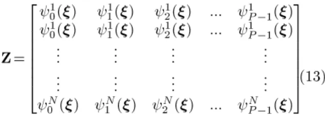
coecients, and Z (Hermit polynomial matrix) is a space-independent matrix of dimension N P and is given as follows:
Z= 2 6 6 6 6 6 6 4
1
0() 11() 12() ::: 1P 1() 1
0() 11() 12() ::: 1P 1()
... ... ... ... ... ... ... ...
N
0 () 1N() 2N() ::: NP 1()
3 7 7 7 7 7 7 5(13)
It should be mentioned that the number of collo-cation points selected should ensure that ZT:Z is
invertible. Flowchart of the SRSM is presented in Figure 1.
5. Random nite-element method
The RFEM is one of the most accurate, yet time expensive, methods to analyze reliability of nite-element models. In this method, a random eld of soil
properties is generated and then mapped onto a nite-element mesh [7]. The steps of this method using K-L expansion are as follows:
1. Representing the statistical properties of stochastic input variables, such as mean, standard deviation, autocorrelation function, and distribution type;
2. Generating random eld using K-L expansion;
3. Performing nite-element analysis using generated random eld to compute system response;
4. Repeating steps 2 and 3 many times using MCS to obtain the histogram of system response;
5. Computing the statistical properties of system response such as mean, standard deviation, and probability of failure (Pf).
The owchart of this method is shown in Figure 2.
6. Computer program
In this study, for reliability analysis of foundation settlement, two nite-element programs were coded by MATLAB based on SRSM, RFEM. These programs are capable of considering the uncertainties of soil
parameters. The major capabilities of these programs are as follows:
1. Considering elastic-perfectly plastic behavior of the soil material with Mohr-Coulomb yield criterion;
2. Selecting appropriate collocation points automati-cally (SRSM program);
3. Generating random eld by K-L expansion consid-ering cross correlation between stochastic parame-ters;
4. Computing chaos polynomials for any number of random variables based on closed-form expressions (SRSM program).
7. Verication of the developed programs To verify the accuracy of the developed programs, a deterministic analysis was done using mean values of soil parameters, given in Table 1. The obtained result, including the foundation pressure-settlement curve, is compared with the prediction result of nite-element software, PLAXIS. For this purpose, soil mass with 13 m width and the depth of 7 m is discretized into 52 four-node rectangular elements in the horizontal direction by 5 elements in vertical direction, as shown in Figure 3. The nodes on the bottom boundary are xed and both lateral boundaries are assumed roller. A strip footing with a width of B = 3:0 m is located on a c soil layer. A uniform footing pressure equal to 150 kPa is applied onto the top of soil layer.
The ultimate settlements at the center of footing
Table 1. Arbitrary selected soil parameters for modelling.
Parameter Value
Young's modulus E (MPa) 30 Poisson's ratio v 0.3 Cohesion c (kPa) 20 Friction angle (deg.) 25 Dilation angle (deg.) 0 Unit weight (kN/m3) 0
Figure 3. Finite element model of soil mass.
Figure 4. The foundation pressure-settlement curves obtained using developed program and PLAXIS.
(Sc) due to the applied pressure using the developed program and PLAXIS were obtained as 0.0198 m and 0.0193 m, respectively. The results show that the devel-oped program can predict settlement with reasonable accuracy. The foundation pressure-settlement curves obtained using the developed program and PLAXIS are shown in Figure 4. This gure shows that the results are close to each other, and the developed program successfully predicted the foundation settlement.
8. Illustrative example
To compare the proposed methods in reliability analy-sis of foundation settlement with others, an illustrative example with arbitrary data is presented. In this example, the elastic-perfectly plastic Mohr-Coulomb yield criterion is adopted to represent the stress-strain behavior of the soil. The mean of soil parameters is selected as in Table 1, and the geometry of problem is considered as in Figure 3. The values of soil parameters are selected arbitrarily.
Only soil elastic properties E and v are considered as uncertain parameters [6,7,27,34] and modeled as cross correlated lognormal random elds. There is no sucient information about coecient of variation of Poisson's ratio. Some authors have suggested that the variability of this parameter can be neglected, while others proposed a very limited range of variability [11]. In this research, Coecient Of Variation (COV) of v is selected equal to 0.05 as Youssef Abdel Massih [35] and COV of E is selected equal to 0.3. A value of {0.5 is used for RE;v [35].
The K-L expansion is employed to discretize random eld. The type of autocorrelation functions of uncertain parameters can be dierent from each other, but in this example, it is assumed that both
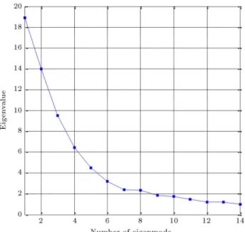
Figure 5. Eigenvalues of 2-D autocorrelation function.
stochastic parameters have the same autocorrelation function as in Eq. (1). It should be emphasized here that the autocorrelation function and autocorrelation length are generally site-specic and often challenging due to insucient site data and high cost of site investigations [11]. Random eld is calculated at the centroid of each element. The rst 14 eigenvalues of 2D autocorrelation function, where values of lx =
20 m and ly = 1 m are considered for horizontal
and vertical autocorrelation lengths, respectively, are shown in Figure 5. In this example, in all cases, 6 terms of K-L expansion are considered rst.
Analyzed by SRSM, polynomials chaos of order 2 is adopted. As nonlinearity of problem is increased, the greater order of polynomials chaos must be selected. Eigenvalues and eigenfunctions of autocorrelation func-tion are computed, and the rst 6 terms of K-L expansion (the rst 6 Eigenvalues and eigenfunctions of autocorrelation function) of each spatial random variable (E and v) are considered. Number of unknown coecient, which must be evaluated, is 91; therefore, 91 collocation points are needed. 106 collocation points are selected, greater than the number of the needed collocation points for the robust estimation of unknown coecients. After computing the unknown coecients, MCS with 100,000 sampling is applied to meta-model (Eq. (9)). The histogram and tted PDF of center of foundation settlement (Sc) determined using SRSM are shown in Figure 6.
In stochastic analysis, using RFEM, eigenvalues and eigenfunctions of autocorrelation function are com-puted rst, and like SRSM, the rst 6 terms of K-L expansion are considered. The random eld has been generated 10,000 times, and the results are used in original nite-element model to determine the Sc.
Figure 6. The histogram and PDF of Sc obtained using SRSM.
Figure 7. The histogram and PDF of Sc obtained using RFEM.
The histogram and tted PDF of the Sc determined using RFEM are shown in Figure 7. For comparing the determined PDF and Cumulative Distribution Function (CDF) by two methods, they are plotted in one gure. Figures 8 and 9 show the determined PDF and CDF of two methods, respectively. These gures show that the results of two methods are close to each other; however, the computational time of the SRSM is considerably less than RFEM.
By assuming the threshold value of footing center settlement equal to 0.025 m and the required time of two methods, the probability of system failure (Pf)
is given in Table 2. It can be seen that the results of SRSM are close to those of RFEM; however, the
Figure 8. The PDFs of Sc obtained using SRSM and RFEM.
Figure 9. The CDFs of Sc obtained using SRSM and RFEM.
consumed time in RFEM is at most 50 times longer than that of SRSM.
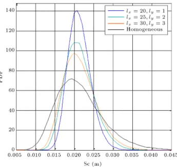
In this study, the eect of autocorrelation length on PDF of system is investigated. For this purpose, the SRSM with less computational time is used. The PDFs of system response for dierent values of autocorrela-tion length and homogenous soil layer (lx= 1; ly= 1)
are shown in Figure 10.
This gure shows that as the autocorrelation
Table 2. Comparison of results of SRSM and RFEM.
Method Sc Sc Pf (%) Time (hour)
SRSM 0.0213 0.0029 10.29 6.80 RFEM 0.0212 0.0029 10.04 360.5
Figure 10. The PDFs of Sc for dierent values of autocorrelation lengths obtained by SRSM.
Figure 11. Pf for various COVs of E by assuming the threshold value of Sc equal to 0.025 m.
lengths increase, the system response dispersion in-creases too and the case of homogenous soil has maximum dispersion. In this analysis, COVs of v and E are selected equal to 0.05 and 0.30, respectively.
The COV and Pf of Sc for dierent values of
autocorrelation lengths are presented in Table 3. From this table, it can be seen that in this example, both Pf
and COV increase with an increase in autocorrelation lengths, and Pf and COV show the largest values for
homogenous soil.
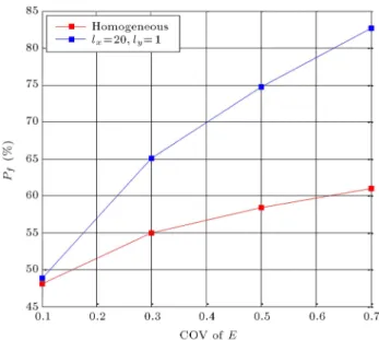
Figures 11 and 12 summarize the variations of the probability of failure with the coecient of variation of E for both cases of ignoring and considering spatial variation of stochastic parameters. These gures show
Table 3. Pf and COV of Sc for dierent values of autocorrelation lengths. Parameter lx= 20 m,
ly = 1 m
lx= 25 m, ly= 2 m
lx=30 m,
ly= 3 m Homogenous
Pf (%) 10.29 16.18 19.07 24.7
COV 0.1345 0.1747 0.1986 0.2837
Figure 12. Pf for various COVs of E by assuming the threshold value of Sc equal to 0.02 m.
the results of two values of threshold footing center set-tlement: 0.025 m (Figure 11) and 0.020 m (Figure 12). This gure shows that the probability of failure increases with increasing COV of E. Figure 11 shows that for COVs of E smaller than 0.7, the predicted Pf of homogenous soil is greater than when spatial
variability is considered, whereas Figure 12 does not show these results. Based on these gures, it can be concluded that to have a correct result in stochastic analysis, it is necessary to consider the spatial variabil-ity of soil properties.
9. Conclusions
In this study, the reliability analysis of foundation settlement by SRSM and RFEM was presented. For this purpose, two nite-element programs were coded by MATLAB based on two methods. The elastic soil properties were considered as spatial random variables and modeled as cross correlated log normal random eld. The results of two methods were compared with each other, and it is observed that the results of two methods are close to each other. In the presented example, to reach the same result, in RFEM, the deterministic numerical model must be run 104 times, while SRSM model must be run 106 times. It is concluded that the SRSM is more time ecient
compared with RFEM, because in SRSM, MCS is applied onto meta-model, whereas in RFEM, the MCS is applied onto the original numerical model, which is more time-consuming compared with meta-model. The eect of autocorrelation length was investigated by SRSM. It was shown that in stochastic analysis, to have a correct result, it is necessary to consider the spatial variability of soil properties.
The approximate real soil behavior, which in-cludes hardening or softening, has not been considered in this research. The authors suggest the following fu-ture studies for further improvements on and extension to the topic:
Three-dimension analysis of foundation settlement by SRSM.
Stochastic analysis of dierential settlement.
Stochastic analysis of settlement problems with seismic or dynamic loading.
References
1. Chau, K.W. \Reliability and performance-based de-sign by articial neural network", Adva. Eng. Soft., 38, pp. 145-149 (2007).
2. Cheng, C.T., Li, X.Y. and Chau, K. \A parallel adap-tive metropolis algorithm for uncertainty assessment of Xinanjiang model parameters", IAHS-AISH publi., pp. 10-16 (2008).
3. Maheshwari, P. \Settlement of shallow footings on layered soil: State-of-the-art", Int. J. Geot. Eng., 9, pp. 42-48 (2015).
4. Dodagoudar, G. and Shyamala, B. \Finite element reliability analysis of shallow foundation settlements", Int. J. of Geo. Eng., 9(3), pp. 316-26 (2015).
5. Fenton, G.A. and Griths, D. \Statistics of block conductivity through a simple bounded stochastic medium", Wate. Resou. Res., 29, pp. 1825-1830 (1993).
6. Fenton, G.A. and Griths, D. \Probabilistic foun-dation settlement on spatially random soil", J. of Geotech. and Geoen. Eng., 128(5), pp. 381-390 (2002).
7. Griths, D. and Fenton, G.A. \Probabilistic settle-ment analysis by stochastic and random nite-elesettle-ment methods", J. Geot. Geoen. Eng., 135, pp. 1629-1637 (2009).
8. Johari, A., Rezvani Pour, J. and Javadi, A. \Reliability analysis of static liquefaction of loose sand using the random nite element method", Eng. Comp., 32(7), pp. 2100-2119 (2015).
9. Paice, G., Griths, D. and Fenton, G.A. \Finite element modeling of settlements on spatially random soil", J. Geot. Eng., 122(9), pp. 777-779 (1996).
10. Pieczynska-Kozlowska, J., Pula, W. Griths, D. and Fenton, G. \Inuence of embedment, self-weight and anisotropy on bearing capacity reliability using the random nite element method", Comp. Geot., 67, pp. 229-238 (2015).
11. Ahmed, A. \Simplied and advanced approaches for the probabilistic analysis of shallow foundations", Nantes (2012).
12. Berveiller, M., Sudret, B. and Lemaire, M. \Stochastic nite element: a non intrusive approach by regression", Eur. J. Comp. Mech., 15, pp. 81-92 (2006).
13. Huang, S., Liang, B. and Phoon, K. \Geotechnical probabilistic analysis by collocation-based stochastic response surface method: An Excel add-in implemen-tation", Geori., 3(2), pp. 75-86 (2009).
14. Huang, S., Mahadevan, S. and Rebba, R. \Collocation-based stochastic nite element analysis for random eld problems", Prob. Eng. Mech., 22(2), pp. 194-205 (2007).
15. Isukapalli, S., Roy, A. and Georgopoulos, P. \Stochas-tic response surface methods (SRSMs) for uncertainty propagation: application to environmental and biolog-ical systems", Ris. anal., 18(3), pp. 351-363 (1998).
16. Jiang, S.H., Li, D.Q., Zhang, L.M. and Zhou, CB. \Slope reliability analysis considering spatially vari-able shear strength parameters using a non-intrusive stochastic nite element method", Eng. geol., 168, pp. 120-128 (2014).
17. Li, D., Chen, Y., Lu, W. and Zhou, C. \Stochastic response surface method for reliability analysis of rock slopes involving correlated non-normal variables", Comp. Geot., 38(1), pp. 58-68 (2011).
18. Li, H. and Zhang, D. \Probabilistic collocation method for ow in porous media: Comparisons with other stochastic methods", Wat. Reso. Rese., 43(W09409), pp. 44-48 (2007).
19. Soubra, A.H. and Mao, N. \Probabilistic analysis of obliquely loaded strip foundations", Soi. foun., 52(3), pp. 524-538 (2012).
20. El-Ramly, H., Morgenstern, N. and Cruden, D. \Prob-abilistic slope stability analysis for practice", Can. Geot. J., 39(3), pp. 665-683 (2002).
21. Lacasse, S. and Nadim, F. \Uncertainties in character-ising soil properties", Publ.-Norg. Geot. Inst., 201, pp. 49-75 (1997).
22. Vanmarcke, E., Random Fields: Analysis and Synthe-sis, MIT Press, Cambridge, MA (1983).
23. Baecher, G.B. and Christian, J.T., Reliability and Statistics in Geotechnical Engineering, John Wiley & Sons (2005).
24. Sudret, B. and Der Kiureghian, A. \Stochastic nite element methods and reliability: a state-of-the-art report", Berkeley, CA: Dep. Civ. Env. Eng., Uni. Cali. (2000).
25. Ghiocel, D.M. and Ghanem, R.G. \Stochastic nite-element analysis of seismic soil-structure interaction", J. Eng. Mech., 128(1), pp. 66-77 (2002).
26. Ghanem, R.G. and Spanos, P.D. \Spectral Stochastic Finite-Element Formulation for Reliability Analysis", J. Eng. Mech., 117(10), pp. 2351-2372 (1991).
27. Ghanem, R.G. and Spanos, P.D., Stochastic Finite Elements: A Spectral Approach, Courier Corporation (2003).
28. Zhang, D. and Lu, Z. \An ecient, high-order per-turbation approach for ow in random porous media via Karhunen-Loeve and polynomial expansions", J. Comp. Phys., 194(2), pp. 773-794 (2004).
29. Cho, S.E. and Park, H.C. \Eect of spatial variability of cross-correlated soil properties on bearing capacity of strip footing", Int. J. Num. Anal. Meth. Geom., 34(1), pp. 1-26 (2010).
30. Vovechovsky, M. \Simulation of simply cross corre-lated random elds by series expansion methods", Struc. Saf., 30(4), pp. 337-363 (2008).
31. Sudret, B. \Polynomials chaos expansions and stochas-tic nite element methods", Ris. Reli. Geot. Eng., (Chapter 6), pp. 265-300 (2015).
32. Tatang, M.A., Pan, W., Prinn, R.G. and McRae, G.J. \An ecient method for parametric uncertainty analysis of numerical geophysical models", J. Geoph. Rese.: Atmospheres (1984-2012), 102, pp. 21925-21932 (1997).
33. Webster, M.D. Tatang, M.A. and McRae, G.J. \Ap-plication of the probabilistic collocation method for an uncertainty analysis of a simple ocean model" , MIT joint program on the science and policy of global change report series no. 4, Massachusetts Institute of Technology (1996).
34. Babu, G.S. and Srivastava, A. \Reliability analysis of allowable pressure on shallow foundation using response surface method", Comp. Geot., 34(3), pp. 187-194 (2007).
35. Youssef Abdel Massih, D.S. and Soubra, A.H. \Reliability-based analysis of strip footings using re-sponse surface methodology", Int. J. Geom., 8(2), pp. 134-143 (2008).
Biographies
Ali Johari obtained his BS, MS, and PhD degrees in 1995, 1999, and 2006, respectively, from Shiraz
University, Iran, where he is currently an Assistant Professor in the Civil and Environmental Engineering Department. He was a Post-Doctoral Researcher at Exeter University in 2008, where he is also a member of the research sta of the Computational Geomechanics Group. His research interests include unsaturated soil mechanics, application of intelligent systems in geotechnical engineering, probabilistic models and re-liability assessment. He has also consulted and
super-vised numerous geotechnical projects.
Abouzar Sabzi was born in Abdanan, Iran, in 1990. He received his BS degree in Civil Engineering from the Ilam University, Ilam, Iran, in 2012. He is studying Geotechnical Engineering at Shiraz University of Technology to obtain MS degree. His current main interests of research are numerical methods and stochastic analysis in geotechnical engineering.