Multivariable Generalized Predictive Control Using An Improved Particle Swarm Optimization Algorithm

Multivariable Generalized Predictive Control Using an Improved

Particle Swarm Optimization Algorithm

Moussa Sedraoui and Samir Abdelmalek

Laboratoire (PI : MIS) Problèmes Inverses: Modélisation, Information et Systèmes, Université 08Mai 1945, Guelma, Algérie

E-mail: [email protected]

Sofiane Gherbi

Laboratoire d’Automatique de Skikda (LAS), Université 20 Aout1955, Skikda, Algérie E-mail: [email protected]

Keywords:improved particle swarm optimization, multivariable generalized predictive control, feasible region

Received:November 16, 2010

In this paper, an improvement of the particle swarm optimization (PSO) algorithm is proposed. The aim of this algorithm is to iteratively resolve the cost problem of the Multivariable Generalized Predictive Control (MGPC) method under multiple constraints previously reduced. An ill-conditioned chemical process modelled by an uncertain Multi-Input & Multi-Output (MIMO) plant is controlled in order to verify the validity and the effectiveness of the proposed algorithm. The performances obtained are compared with those given by the MGPC method using the standard PSO algorithm. The simulation results shows that the proposed algorithm outperforms standard PSO algorithm in terms of performance and robustness.

Povzetek: Predstavljena je metoda optimiranja z roji za nadzor s splošnim napovedovanjem in več spremenljivkami.

1

Introduction

Multivariable generalized predictive control (Morari & Lee, 1999) is a very powerful method. It has been the subject of many researches during the last few years and it was applied successfully in industry, particularly in chemical processes. It is based on MIMO predictive model [1], [2] where the expected behaviour of the system can be predicted in the extended time horizon. The MGPC law is obtained by minimizing linear or non-linear criterion (Magni, 1999, Duwaish, 2000). This criterion is composed by the sum of the square prediction errors between the predicted and desired outputs, the weighted sum of the square change-controls (control-increments) and others [3]. The constraints inclusion (as mathematical inequalities type) distinguishes most clearly MGPC from other process control paradigms as suggested in (Richalet, 1993, Qin 1997, Rawlings, 1999). These constraints are imposed in order to ensure a better stability and performance robustness (Al Hamouz and Duwaish, 2000, Imsland, 2005). The MGPC method formulates the constraint optimization problem at every step time for solving the optimal control move vector [4]. At the next sampling time, a new process measurement is received, the process is updated, and a new constraint optimization problem is solved for the next control move vector. An efficient randomized constraint optimization algorithm is suggested to the MGPC method named by

improve the performances of the MGPC method. The first one consists to reduce (if possible) the imposed inequality constraints which are reformulated as boundary constraints. The second one is to resolve the bounds constraints optimization problem by the improved PSO algorithm.

2

Unconstrained MGPC Method

All the considered matrices are in discrete time domain. A CARIMA (Controller Auto Regression Integrated Moving Average) model for an minputs and moutputs multivariable process can be expressed by [8]:

) ( ) ( ) 1 ( ) ( : ) ( )

(q 1 yt B q 1 ut C q 1 t

A  _{ }  _{  }  

(1) Where





T

m

m _{y t y t y t}

t

y() 1: ₁( ) ₂() ... ()





T

m

m _{u t u t u t}

t

u() 1: ₁() ₂() ... () )

(q1

A ,B(q1)and C(q1)are mmmonic polynomial matrices. Set C(q1)equal to the unity diagonal matrix. (t)is an uncorrelated random process and (q1)1q1, this form enables to introduce an integrator in the control law. Without lost of generality one can suppose A as diagonal polynomial matrix.

 

) (t

y_i , u_i(t) denotes respectively, the process output and the control input of the channel

number ‘i’. q1denotes the backward shift operator. The role of (q1)is to ensure an integral action of controller in order to cancel the effect of the step varying output in the channel ‘i’.

As in all receding horizon predictive control strategies, the control law provides that, for each channel ‘i’, the control-increment u_i(t)which minimizes the following unconstraint cost problem of the MGPC method [8]:









 



                   m i N j N j i i i i i i u j t u j t w t j t y J

1 1 1

2 2 2 ) 1 ( ) ( ) / ( ˆ :  (2) Where    ) ( ˆ t j

y_i is an optimum j-step-ahead prediction of the system output vector on data up to time t, therefore, the expected value of the output vector at time tif the past input vector, the output vector, and the future control sequence are known. Noting thatyˆ_i(t j) is depending to the control-incrementu_ifrom resolving two Diophantine equations (more details are available in the reference [9]).

 

) (t

w_i is the future set-point or the reference sequence for the output y_i(t).

i

N₂, N_ui(with respect:N_ui N₂i) denotes respectively, the maximum output prediction horizon

(assumed equal toN₂) and the maximum control prediction (assumed equal toN_u) for each channel

‘i’. _idenotes the positive parameter weighting the control input for each channel ‘i’.

3

Classification of Constraints and

Problem Formulation

In constrained control, a set of inequality constraints may be set as addition of the control objective and the variation limits of certain variables to the given ranges:

i i

i v t j v

v  (  ) , with i:1,2,..m and

2 1,..., : N_s N_s

j  .

Where

   ) (t j

v_i is a variable under restriction,

 

i

v andv_iare the lower and the upper boundaries,

1 s

N andN_s2are the lower and the upper constraint horizons respectively.

The two main objectives of constrained predictive control are set-point tracking and prevention / reduction of constraint transgressions. These constraints can be imposed (with respect to the time index) on the control-increment vector, or/and on the control vector as follows:

- Constrained on the control-increment:

i i

i u t j u

u   

 ( ) (3) Where i1,2,..m andj0,...,N_u1.

- Constrained on the control:

i i

i u t j u

u  (  )

(4) Where i1,2,..m andj0,...,N_u1.

By using:



       j k i i

i t j u t u t k

u 0 ) ( ) 1 ( : )

( (5)

The control constraints (4) becomes as follow:



         j k i i i i

i u t u t k u u t

u 0 ) 1 ( ) ( ) 1

(

(6)

The constraints on the control vector and the rate of control changes, with respect to the batch index, can be easily combined together:

inq

inq U B

A   (7) Where                     _{ } ) 1 ( ) 1 ( ) ( : 1 ) ( u N m N t U t U t U U _u

 denotes the design

parameter vector which will be determined later by the PSO algorithm, it contains the future control- increment vector





1

)

(  _

U t j m of each channel as:

 

A_inq (4.m.Nu)(m.Nu),

 

1 ) . . 4 ( mNu inq

B are defined by:

                   ) ( ) ( ) ( ) ( : m m m m m m m m inq I tril I tril I diag I diag A Where ) . ( ) . ( )

( mNu mNu m

m I

diag _   denotes the unity diagonal

matrix, and ( ) (m.Nu) (m.Nu) m

m I

tril _   denotes the lower triangular matrix of the unity diagonal matrix(I_mm).

 

 









                              1 ) ( 1 ) ( 1 ) ( 1 ) ( ) 1 ( ) 1 ( : u u u u N m i i N m i i N m i N m i inq t u u t u u u u B

The cost index (2) can be expressed in matrix form as: 0 1 2 : ) ,

( U t U Q U Q U Q

J   T   T  (8) WhereQ₂:GTG, Q₁T :2



W



TG and



W

 

W



Q₀:  T  ) ( ) ( : u u mN N m I _{  }

 

  is diagonal matrix weighting the control-increment vector, and _{( )1}

2 N m

W is the

projected set-point vector.

) ( ) (mN2 mNu

G _{  } , _{( )1}

2 

mN are the polynomial matrices which are determined by the recursively resolution of the two Diophantine equations [9].

The cost index (8) and the inequality constraints (7) formulate the following constraint optimization problem as:                   inq inq T T U B U A Q U Q U Q U t U J : s.t : ) , (

min _{2 1 0}

(9)

Now, an optimal control vector is given by the PSO algorithm. This algorithm should minimize the objective function (8) under4mN_uinequality constraints. The computational requirements of the PSO algorithm depend heavily on the number and the type of the constraints to be satisfied. An efficient off-line constraint PSO algorithm, suggested by Ichirio & al, 2009, can resolve this problem [10]. Unfortunately, this algorithm is difficult to extend to the MGPC method for two reasons: the first one is due to a large dimension of the inequality constraints which needs excessive computation time. The second one is due to a real-time output feedback implementation of the MGPC method which requires a minimum consuming time. To resolve these above problems, the inequality constraints should be reduced, for each step time, and reformulated as bounds constraints type. Only those constraints (which limit the feasible region) must be taken into account. The efficiency of the PSO algorithm can be increased if the superfluous constraints (which do not limit the feasible region) should be eliminated [11]. In this paper we

propose a systematic method that determines the minimum set vector of limiting constraints. The lower and the upper bounds of the feasible region are given as below:

For each channel i:1,,m, the control-increment )

(t u_i

 is simultaneously constrained by: 1- For the control prediction horizonj0:

                ) 1 ( ) ( ) 1 ( ) ( t u u t u t u u u t u u i i i i i

i

₍₁₀₎

It is easy to see that the new lower and upper bounds are determined by: ) ( ) ( )

(t u t v t

vi  i  i (11) Where } ) 1 ( max{ : )

(t  u u u t

v_{i i i} (12) } ) 1 ( min{ : )

(t  u u ut

vi i i (13) 2- For the control prediction horizon j1:

                    ) 1 ( ) ( ) 1 ( ) 1 ( ) 1 ( t u u t u t u t u u u t u u i i i i i i i

(14)

The new lower and upper bounds are determined for 1  j by: ) 1 ( ) 1 ( ) 1

(t u t v t

v_{i i} i

(15) Where )} ( )} 1 ( { max{ : ) 1

(t u u u t v t

v_i    _{i i}   _i (16)

)} ( )} 1 ( { min{ : ) 1

(t u u ut v t

v_i    i i   i

(17) This procedure is repeated until the control prediction horizonjN_u1. Therefore the control-increment

) 1

(  

u_i t N_u is constrained by the new bounds:

} ) ( )} 1 ( { max{ : ) 1 ( 2 0



        

 Nu

k i i

i u

i t N u u ut v t k

v (18) } ) ( )} 1 ( { min{ : ) 1 ( 2 0



        

 Nu

k i i

i u

i t N u u ut v t k

v

(19) Then, for each step time valuet₀,t₁,,t_max, the feasible region

m ij N i

i t j v t j u

v t j i D , , 1 1 , , 0 ) ) ( ) ( ( : ) , , (     

 can be

determined by the following proposed algorithm:

3.1

Reduced constraints algorithm

For each point timet₀,t₁,,t_max, the feasible region is determined by the followings steps:

[Step 1]: Set the first counter i1which denotes the number of channels, and go to the next step.

[Step 2]:Set the second counterj0which denotes the control horizon prediction, and go to the next step.

[Step 3]:Set the parametersh_max0, h_min 0and go to the next step.

[Step 4]:Build the followings ranges: } )} 1 ( { { : max

_ u u u t h_max

} )} 1 ( { { : min

_ u u u t h_min

bound i   i i i   .

[Step 5]: Calculate the new upper and the new lower bounds which limit the control- increment u_i(t j)by:

} max _ min{ : ) ( i

i t j bound

v  

} min _ max{ : ) ( _i

i t j bound

v  

From these above bounds, the feasible region is determined as follow:

) ) ( ) ( ( : ) , ,

(i jt v t j v t j

D  i  i 

[Step 6]:Update the parameters:h_min,h_max as follows )

( max

max h v t j

h   _i 

,

) ( min

min h v t j

h   _i 

,

and go to the next step

[Step 7]: Update the second counter j j1and go back to the step 4 ifjN_u 1. Otherwise, go to the next step.

[Step 8]: Update the first counter ii1and stop algorithm if i:m

.

Otherwise go back to the step 2. From this above algorithm, the constraint optimization problem (9) under inequality constraints is reformulated as the bounds optimization problem:

                    U U U Q U Q U Q U t U

J T T

U : s.t : ) , (

min 2 1 0

(20)

WhereU , U denotes respectively, the new lower and the new upper bounds vector which limit the feasible region D(m.Nu)2:(U,U), with:

 





T

m i u i i i N

m v t v t v t N

U

u)1  1,2

.

(  : () ( 1) (  1) 



 





T

m i u i i

i t v t v t N

v U mNu



 ( 1) _1,2

) 1 ( ) ( : 1 ) . (     _  

From (20), it is easy to see that the inequality constraints number is reduced to mN_uconstraints at each step time. This dramatic reduction has a capital importance for the success of the PSO algorithm.

Now, we are able to find the optimal control of the MGPC law. The new constraint optimization problem (20) should be resolved for each step time

max 1 0, , , : t t t

t   , its solution vectorU*denotes the optimal design parameter vector. Only the first m rows

of U* is used to obtain the optimal desired control-increment vector of each channel (' i '). The optimal control vector is obtained by adding the previous control vector to the optimal control-increment vector as follow:

) ( ) 1 ( : )

(t u t u* t

u_i  _i   _i (21)

4

Improved PSO Algorithm [6]

Particle swarm optimization algorithm, introduced first by Kennedy and Eberhart in (1995), is one of the modern heuristic algorithms which belong to the category of Swarm Intelligencemethod (Kennedy, 2001). The PSO algorithm uses a swarm consisting ofN_pparticles for each control-increment vector





m ij N

i t j _u

u  , 2 , 1 1 , 1 , 0 ) (     to

get an optimal solution u_i*(t j)which minimizes the optimization problem (20). The position of ( ith) particle

and its velocity are respectively denoted as [12]:





T

N i i

i

i t j u t j u t j u t j

u (  ):  ,1(  )  ,2(  )  , _p(  )

 





T

N i i

i

i(t j): ,1(t j)  ,2(t j)  , p(tj)

 

.

Then, the position of the ( ith) particle, ui(tj), is based on the following update law:

for 1,2,max, which indicates the iteration number [12],



 







 



   i best swarm i i best i i i

i c cr H u c2r2, h , u ,

, 1 1 0 1_{: }  (22) 1 1 :   _{ }     i i i u

u  (23) Where c₁and c₂are respectively, the cognitive (individual) and the social (group) learning rates and are both positive constants. The value of cognitive parameter

1

c signifies a particle's attraction to a local best position based on its past experience. The value of social parameterc₂determines the swarm's attraction towards a global best position.

  

0

c is the inertia weight factor whose value decreases linearly with the iteration number (Shi & Eberhart, 1999) as [13]:

  _        max min max max 0:   

c (24)

Where _maxand _minare the initial and the final values of the inertia weight, respectively. The values of

9 . 0 max 

 and min 0.4are commonly used [13]. The random numbersr₁_,iand r₂_,iare uniformly distributed in

 

0,1.



, best i

H andh_swarmbest,denotes respectively, the best previously obtained position of the ( ith ) particle (the

position giving the lower value of the objective criterion) and the best position in the entire swarm at the current iteration  [10]:

} 0 ), ( { min arg : , _{   }

 J u r

H r i u best i r i (25) } ), ( { min arg :

, _{J u i}

h _i u best swarm i      

 (26)

From equation (23), some current position of ( ith)

particle (in each dimension) can exceed the corresponding lower bound or upper bound of the feasible region. Consequently, the given optimal control vector of the MGPC method cannot satisfy some specifications and also some constraints are non-satisfactoriness' in some range time. To avoid, we should improve the convergence of PSO algorithm by adjusting only the corrupted position of ( ith ) particle with the

region around the current established solution, if it is too smaller than the corresponding lower bound, its valuev_i

corresponding upper bound, then its value is replaced by

i

v . The proposed modification can be formulated as follows:

Let consider:

) (t j u_iq 

 : The corrupted position of ( ith) particle

given at current iteration :q. )

(t j

v_i  , v_i(t j): The lower bound and upper bound which are determined by the reduced constraints algorithm. So that, the above corrupted position can be adjusted by using the following inequalities:

               ) ( ) ( : ) ( ) ( ) ( : ) ( : ) ( j t v j t u if j t v j t v j t u if j t v j t u i q i i i q i i q i   (27)

Consequently, from the equation (23), the current velocity should be limited by the following bounds:

1 1   _   q i i q i q i

i u v u

v   (28) Now, the modified current positions with their modified velocity are used to improve the next best position and their velocity vector for the next iteration as follow:







q



i q best swarm q i q i q best i q i q i q

i c cr H u c2r2, h , u , , 1 1 0 1 :   (29) 1 1 :   _{ }  q i q i q i u

u  (30) The improved PSO algorithm consists of the following steps:

4.1

Proposed algorithm

For each step time t:t₀,t₁,,t_maxthe optimal control-increment is determined by the following steps:

[Step 1]:Determine the lower bound and the upper boundv_i(t j),v_i(t j)which are corresponding the

design parameter





1 , , 0 :1, , : ) (      u N j m i i t j u



 .

[Step 2]: Initialize random swarm positions and velocities:

initialize a population (array) of particles with random positions and velocities (array) from the search domainD:(U,U).

Set the counter1and go to the next step.

[Step 3]: Evaluate the objective criterion (20) and obtain best,

i

H , best,

swarm

h according to (25) and (26).

[Step 4]: Update of a particle's velocity and its position according to (22) and (23).

[Step 5]: Check each parameter of the particle's position by the following corresponding lower bound and upper boundv_i(t j),v_i(t j). Replace only those exceeding these above bounds.

[Step 6]:Update the counter 1and go back to the step 3 if max. Otherwise, stop algorithm and

take the best position vector as an optimal solution which minimize the constrained optimization problem (20).

5

Simulation Results and Discussion

In this section, a multivariable generalized predictive control method using a modified particle swarm optimization algorithm is applied to a distillation column which is MIMO plant with two input and output vectors (benchmark problem, see [14]). The two inputs are the reflux and the vapour boil up rate and the outputs are the distillate and the bottom product. The results are compared with those given by the MGPC method using the standard PSO algorithm. The mathematical model is given by [14]:

                

  s _{ s}

e K e K s s G 2 1 2 1 0 0 096 . 1 082 . 1 864 . 0 878 . 0 1 75 1 : ) ( _  (31)



0.8 1.2



) 2 , 1 (i  i

K , _i(i1,2)



0.0 1.0



. Where

i i,K

 denotes respectively, the uncertainty temperatures and uncertainty gains of the process.

The time domain specifications are formulated, for the time range t



0,400



minutes, as below:

a- For the first set-point reference vector:w



1 0



T , the first and the second output channelsy₁andy₂must satisfy[14]:

(S1):y1(t)0.9in more than 30 minutes.

(S2):y1(t)1.1: the maximum over-shoot corresponding the first output channel cannot exceed 11% for all range timet



0,400



.

(S3):0.99y1()1.01: the static error value cannot exceed 1% ( y₁()w₁() 1%).

(S4):y2(t)0.5: the maximum over-shoot of the second output channel cannot exceed to 50% for all range timet



0,400



.

(S5):For t:0.01y2(t)0.01: the static error value cannot exceed 1%. From another word:

% 1 ) ( ) ( ₂

2  w  

y .

(S6):Closed loop stability.

(S7):Control signals should be limited by



200 200



.

(S8):Control-increment signals should be limited by



12 12



.

For the set-point reference vector: w



1 0



T, the sampling timeT_e 1minute is used to determine a CARIMA predictive model of the chemical process for two followings parameters cases [14]:

1 2 , 1 2 ,

1  

K andK₁1.2,K₂ 0.8,_1,2 1.

b-The same previous time domain specifications should be satisfied for the second set-point reference

The MGPC method is tuned by choosing: )

01 . 0 , 6 , 8 ( ) , ,

(N₂i N_ui _{i i1,2}  at time range t:



0,400



minutes.

For each step time: t:t0,t1,,400, the feasible region is determined from the following constraints:

200 )

( 200

2 , 1

5 , ,

0 

  



ij i t j

u _ .

12 )

( 12

2 , 1

5 , ,

0 

   



ij i t j

u _ .

From the reduced constraints algorithm (see section 3.1), these above inequality constraints are reduced in order to determine the search spaceDat each step time. The constrained optimization problem is resolved by standard

and improved PSO algorithms according to the following parameters:

- Swarm size: Np:24.

- Maximum iteration: _max:100.

- Cognitive and social learning rates: c₁c₂:1. For the set-point reference vector:w



1 0



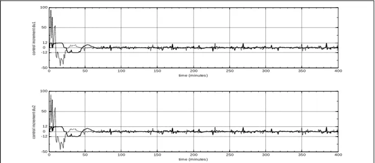
Tand the parameter system’s:K_1,2 _1,2 1, the figures 1.1 to 1.3 shows the results given by the MGPC method using the standard PSO algorithm (dashed curves), and the MGPC method using the improved PSO algorithm (line curves). The table1 summaries the results obtained by the two algorithms.

Figure 1.1: Set-point tracking results with standard and improved PSO algorithms forw



1 0



TandK_1,2 _1,21.

Figure 1.2: Control effort results with standard and improved PSO algorithms forw



1 0



Tand K1,2 1,21.

0 30 50 100 150 200 250 300 350 400

0 0.2 0.4 0.6 0.9 1 1.1

tim e (m inutes )

o

u

tp

u

t y

1

0 50 100 150 200 250 300 350 400

-0.2 0 0.2 0.5

tim e (m inutes )

o

u

tp

u

t y

2

0 50 100 150 200 250 300 350 400

-100 0 100 200 300 400

tim e (m inutes )

co

n

tr

o

l e

ffo

rt

u

1

0 50 100 150 200 250 300 350 400

-100 0 100 200 300 400

tim e (m inutes )

co

n

tr

o

l e

ffo

rt

u

Figure 1.3: Control-increment results with standard and improved PSO algorithms forw



1 0



TandK_1,2 _1,21.

Specifications (Sk):

Algorithms: (S1) y1(30)

(S2) (S3)

y1(400)

(S4) (S5)

y2(400)

(S6) stable

/ unstable

(S7) Unsatisfactory/

satisfactory constraints

(S8) Unsatisfactory/

satisfactory constraints

Decision & reasons

max(y1) time max(y2) time

Standard PSO

1.010 1.074 23 1.010 0.343 8 0.006864 stable unsatisfactory

-9.1≤u1≤349.3

-9.9≤u2≤351.4

unsatisfactory -44≤Δu1≤93 -44≤Δu2≤91

Rejected algorithm

(S7),(S8)

Improved PSO

0.990 1.096 40 0.9975 0.4846 13 0.002512 stable Satisfactory

-20.1≤u1≤200

-20.3≤u2≤199

Satisfactory

-12≤Δu1≤12

-12≤Δu2≤12

Accepted algorithm

Table 1: Summary of the results (unsatisfactory performances are in bold) for the nominal model and the set-point

referencew



1 0



T.

According to the figure 1.1, we can see that, the tracking dynamic of set-point reference vector found by MGPC method based on a standard PSO algorithm is better than the other algorithm but unfortunately, the time domain specifications: (S7) and (S8) are not satisfied.

In the figure 1.2, the obtained control signals of the MGPC method based on standard PSO algorithm exceed the constraint ranges at t:



5,6,15



minutes such as:

3 . 349 ) 9 ( max

1 

u and u_2max(9)351.4. In addition, the control-increment signals presented in the figure 1.3 also violate the constraint ranges at times:



 

 





2 5, 7 11,13 22



:   

t minutes.

Consequently, the performance robustness of this method is very poor in comparison with the MGPC method using the improved PSO algorithm which is capable to satisfy all time domain specifications. These results confirm the usefulness and the robustness of the proposed algorithm.

Figures 2.1, 2.2, 2.3 and table 2 give the results of the MGPC method with the following parametric changes in the process:



K11.2,K20.8,1,21



for the set-point reference vectorw



1 0



T.

According to the figures 2.1 to 2.3, the better results are obtained by the improved PSO algorithm which satisfies all time specifications (S1 to S8). These results can be

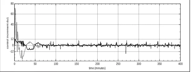
explained by the best stability robustness against the process parametric disturbances. Furthermore, the control and the control-increment signals from the standard PSO algorithm show a dramatic oscillation at transient time region and exceed the constraint ranges. In fact, this algorithm cannot fulfill the three followings time domain specifications: (S2) withmax(y1)11.124%, (S7) with

251 max

1 

u ,u_2max374and(S8)with

76 . 70 4

.

26  1

 u , 39.7u2 99.05, which can be explained by a high sensitivity to the parametric process variations. Thus, from these figures and table 2, we confirm the superiority of the proposed algorithm.

Figures 3.1, 3.2, 3.3 and table 3 give the results of the MGPC method using both algorithms when low gains directions of the process and set-point reference vector

change simultaneously as follows:



K10.8,K2 0.8,1,2 1



,





T

w 0 1 .

0 50 100 150 200 250 300 350 400

-50 -12 0 12 50 100

tim e (m inutes )

co

nt

ro

l i

nc

re

m

en

t d

u1

0 50 100 150 200 250 300 350 400

-50 -12 0 12 50 100

tim e (m inutes )

co

nt

ro

l i

nc

re

m

en

t d

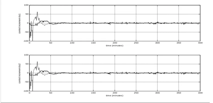
These above figures clearly show the performance superiority of the proposed PSO algorithm over standard PSO. For this case, the time domain specifications: S2 , S7

and S8 are satisfied with the proposed PSO algorithm,

while the same specifications are not satisfactoriness with standard PSO. In addition, the obtained outputs by the standard PSO algorithm converge to the set-point references but unfortunately, two other specifications cannot be satisfied at time t  208 minutes which are:

(S3): y2(208)w2(208) 5%. (S5): y1(208)w1(208) 3%.

6

Conclusion

In this study, we proposed an improvement of the PSO algorithm, it has been introduced and applied to solve the

constrained MGPC problem. In order to find a feasible region, the constraints on the controls and their increments have been previously reduced at each step time, the obtained convergences by improved PSO algorithm are well improved in comparison with the standard PSO algorithm. The efficient of the proposed algorithm is clearly shown and the performances robustness and the stability robustness are guaranteed with little still sensitivity to a set-point references changes and parametric model uncertainties. The results of the proposed algorithm justifies its efficiency and presents quite promising results and can be a subject of an interesting investigations.

Figure 2.1: Set-point tracking results with standard and improved PSO algorithms for w



1 0



Tand



K₁1.2,K₂ 0.8,_1,21



.

Figure 2.2: Control effort results with standard and improved PSO algorithms for w



1 0



Tand



K₁1.2,K₂ 0.8,_1,21



.

0 30 100 150 200 250 300 350 400

0 0.1 0.3 0.5 0.9 1 1,1

tim e (m inutes )

ou

tp

ut

y

1

0 50 100 150 200 250 300 350 400

-0.2 0 0.2 0.4 0.5

tim e (m inutes )

ou

tp

ut

y

2

0 50 100 150 200 250 300 350 400

-200 -100 0 100 200

tim e (m inutes )

co

nt

ro

l e

ffo

rt

u

1

0 50 100 150 200 250 300 350 400

-200 -100 0 100 200 300

tim e (m inutes )

co

n

tro

l e

ffo

rt

u

References

[1] D.W Clarke, C. Mohtadi & P.S Tuffs, Generalized Predictive Control –Part I : The basic algorithm – Part II: extensions and interpretation. Automatica, 23(2), 1987, 137-160.

[2] D.W Clarke & C. Mohtadi, Properties of generalized predictive control, Automatica, 25(6), 1989, 859-875.

[3] P. Codron & P. Boucher, Improvement for multivariable generalized predictive control with multiple reference models. Proc. 12th IASTED International Conf. Modeling. Identification. And Control, Innsbrûck, Austria, Feb.1993.

[4] T.S. Chang & D.E. Seborg, A linear approach programming for multivariable feedback control with inequality constraints, International journal of control 37,1983, 583-597.

[5] M. Zribi, M. Al-Rashed & M. Alrifai. Adaptive decentralized load frequency control of multi-area power systems. Electrical Power and Energy Systems, 27:575583, 2005.

[6] J.P. Coelho, P.B.M. Oliveira & J.B. Cunha. Greenhouse air temperature control using the

particle swarm optimization algorithm. 15th Triennial world congress. Barcelona, Spain. IFAC, 2002.

[7] L.D.S. Coelho & al. Model-free adaptive control optimization using a chaotic particle swarm approach. Chaos, solutions and fractals. Elsevier. 41, 2009, pp2001-2009.

[8] P. Codron & P. Boucher. Multivariable generalized predictive control with multiple reference models: A new choice for the reference model, ECC’93. European Control Conf., June 28- July1993. [9] P. Zelinka, B.R. Ilkiv & A.G. Kuznetsov.

Experimental verification of stabilizing predictive control. Control engineering practice7. 1999, pp 601-610.

[10] I. Maruta, T. Hyoung & T. Sugie: Fixed-Structure



H

Controller: A Meta-Heuristic Approach Using Simple Constrained Particle Swarm Optimization. pp:553-559.Automatica 45(2009).

[11] E.F. Camacho. Constrained Generalized Predictive Control, IEEE Transaction on Automatic Control, AC-38 (2), 1993, 327-332.

Figure 2.3: Control-increment results with standard and improved PSO algorithms for w



1 0



Tand



K11.2,K20.8,1,21



.

Specifications (Sk):

Algorithms: (S1) y1(30)

(S2) (S3)

y1(400)

(S4) (S5)

y2(400)

(S6) stable

/ unstable

(S7) Satisfactory/ unsatisfactory

constraints

(S8) Satisfactory/ unsatisfactory

constraints

Decision for reasons (Sk)

max(y1) time max(y2) time

Standard PSO

1.061 1.1124 24 0.9953 0.2562 8 0.006142 stable unsatisfactory

-19.2≤u1≤251

-29.4≤u2≤374

unsatisfactory

-26.4≤Δu1≤70.76

-39.7≤Δu2≤99.05

Rejected algorithm (S2),(S7),(S8)

Improved PSO

0.920 1.054 40 0.9953 0.493 12 0.006142 stable Satisfactory

-3.5≤u1≤133.5

-6.4≤u2≤199

Satisfactory

-8.38≤Δu1≤12

-12≤Δu2≤12

Accepted algorithm

Table 2: Summary of the results (unsatisfactory performances are in bold) for the uncertainty model



K11.2,K20.8,1,21



and the set-point reference





T

w 1 0 .

0 50 100 150 200 250 300 350 400

-12 0 12 40 60 80

time (minutes)

c

o

n

tr

o

l

in

c

re

m

e

n

t

d

u

[12] H.N. Al-Duwaish, S.Z. Rizvi & al. PSO based Hammerstein modeling and predictive control of non linear multivariable boiler. Control Engineering practice, pp.1-12, 2010.

[13] S. R. Singiresu: Engineering Optimization: Theory and Practice, Fourth Edition, by John Wiley & Sons, Inc. Hoboken, New Jersey. pp:708-714, & pp:761-768, 2009.

[14] D.J.N Limebeer. The specification and purpose of a controller design case study, IEEE Conf. Decision Control, Brighton, U.K, 1991, 1579-1580.

Figure 3.1: Set-point tracking results with standard and improved PSO algorithms forw



0 1



Tand



K10.8,K2 0.8,1,2 1



.

Figure 3.2: Control effort results with standard and improved PSO algorithms forw



0 1



Tand



K₁0.8,K₂ 0.8,_1,2 1



.

0 30 100 150 200 250 300 350 400

-0.2 -0.1 0 0.1 0.2 0.3 0.4 0.5

time (minutes)

o

u

tp

u

t

y

1

0 30 50 100 150 200 250 300 350 400

0 0.2 0.4 0.6 0.9 1.1

time (minutes)

o

u

tp

u

t

y

2

0 50 100 150 200 250 300 350 400

-400 -300 -200 -100 0 100

time (minutes )

c

o

n

tr

o

l

e

ff

o

rt

u

1

0 50 100 150 200 250 300 350 400

-400 -300 -200 -100 0 100

time (minutes )

c

o

n

tr

o

l

e

ff

o

rt

u

Figure 3.3: Control-increment results with standard and improved PSO algorithms forw



0 1



Tand



K10.8,K2 0.8,1,2 1



.

Specifications (Sk):

Algorithms:

(S1) y2(30)

(S2) (S3)

y1(400)

(S4) (S5)

y2(400) (S6) stable

/ unstable

(S7) Satisfactory/ unsatisfactory

constraints

(S8) Satisfactory/ unsatisfactory

constraints

Decision for reasons

(Sk)

max(y2) time max(y1) time

Standard PSO

1.046 1.167 21 0.9985 0.202 8 -0.003 stable unsatisfactory

-379.7≤u1≤56 -383≤u2≤55.3

unsatisfactory -97.7≤Δu1≤62.4 -99.2≤Δu2≤62.5

Rejected algorithm (S2),(S7),(S8)

Improved PSO

1.032 1.10 40 1.005 0.345 12 0.0009 stable Satisfactory

-199≤u1≤20.3

-200≤u2≤19.9

Satisfactory

-12≤Δu1≤12

-12≤Δu2≤12

Accepted algorithm

Table 3: Summary of the results (unsatisfactory performances are in bold) for the uncertainty model



K₁0.8,K₂ 0.8,_1,2 1



and the change set-point referencew



0 1



T.

0 50 100 150 200 250 300 350 400

-100 -50 0 50 100

tim e (m inutes )

co

nt

ro

l i

nc

re

m

en

t d

u1

0 50 100 150 200 250 300 350 400

-100 -50 0 50 100

tim e (m inutes )

co

nt

ro

l i

nc

re

m

en

t d