A Two-stage Algorithm for Outlier Detection Under Cloud Environment Based on Clustering and Perceptron Model

(1)

Available at http://www.Jofcis.com

A Two-stage Algorithm for Outlier Detection Under

Cloud Environment Based on Clustering and Perceptron

Model

Bing HU

1,

∗

, Fuxi ZHU

1

,

Lu LU

2

, Rong GAO

1

1_{School of Computer, Wuhan University, Wuhan 430072, China}

2_{College of Computer Science and Technology, Shanghai University of Electric Power, Shanghai}

200090, China

Abstract

Outlier detection in large high dimensional datasets is an important and difficult branch of outlier detection research. Since large high dimensional datasets are characterized by sparse data distribution and high dimensional attribute, traditional distance-based outlier detection methods cease to be effective when dealing with massive data. And to solve the above mentioned problem, in this paper, we propose MR-ODCDCalgorithm that is a two-stage outlier detection algorithm based on both clustering and perceptron model. MR-ODCDC algorithm first obtains several micro-clustering components by clustering the dataset with K-means clustering algorithm, then mines local outliers from the objects in these micro-clustering components by adopting a method that combines the perceptron model and the distance-based outlier detection algorithm, and finally realizes parallelization and scalability using MapReduce programming model. Experimental results have shown that our algorithm has improved the efficiency of outlier detection technique to some extent. And the larger the dataset is, the more obvious effect our algorithm achieves. In the area of Web services, situational awareness technology is to receive the current trend of service by perceiving Web services. In situational awareness technology, there are two key algorithms, the trend-extraction algorithm and the trend-recognition algorithm. In these two algorithms, three key threshold parameters are proposed. If these three threshold parameters are set too large, the fitting accuracy will be reduced; if too small, it will lead to the concussion of fitting fragment. Therefore, the adaptive threshold setting algorithm by genetic algorithm is proposed in this dissertation. The results of simulation experiments show that this method is able to find the three optimal thresholds which have minimum fitting error and thus is better than the traditional fixed threshold setting method. Keywords: Outlier; MapReduce; Data Mining; Cell; Massive Data; Clustering Analysis

1 Introduction

Outlier detection [1-3], also known as outlier mining, aims at selecting out from a large complex dataset a small part of abnormal data which is novel and diﬀerent from the conventional ones. In

∗_{Corresponding author.}

Email address: [email protected](Fuxi ZHU).

(2)

practical applications, outliers can be classified into two categories: 1) One is brought about by human errors or measuring equipment failure, such as execution error or incorrect measurement. This kind of outliers is useless and is to be eliminate. 2) The other kind is caused by data itself. This kind of outliers are very interesting and usually carry useful information. They are the concern for outlier detection study. Outlier detection has found wide application in such fields as credit card fraud, loan application, network intrusion detection and customers classification, to name a few.

As an important branch of data mining, in recent years, outlier detection has attracted a great deal of attention from many researchers and some promising results have been achieved [4]. There are numerous outlier detection algorithms. They can generally be divided into 5 categories: 1) distribution-based algorithms [5]; 2) depth-based algorithms [6]; 3) density-based algorithms [7]; 4) distance-based algorithms [8]; and 5) clustering-based algorithms [9]. In [8], the authors offer a general distance-based definition for outliers and propose an outlier detection method which can determine whether a data is an outlier without definitive data distribution available by adopting the K-distance neighborhood. But the time complexity of this algorithm is rather high and the mining result is very sensitive to the selection of the parameter. Moreover, the accuracy and timeliness of the detection result will be on decline as the size and dimensionality of the dataset increases. The study in [9] focuses on the discovery of clusters. It first clusters the dataset, and after clustering, the data points left will be labeled as outliers. This method is simple but is of low efficiency. Through the above analysis, we can see that in spite of those many existed outlier detection algorithms, none of them can effectively deal with massive data. And with the rapid development of parallel computing technologies, to improve the detection efficiency in massive data, a new distributed outlier detection algorithm which is based on cloud environment and combines cloud computing technology [10, 11] with outlier detection algorithm is in urgent need. In this paper, we present an outlier detection algorithm based on Hadoop cloud platform. Our algorithm combines the clustering analysis together with the cell-based approach in distance-based outlier detection method [12], and divides the whole algorithm into two subtasks by adopting the parallel programming model of sequential modular MapReduceputting forward by Google company. When detection, the MapReduce programming model is used to realized the subtasks one by one. The feasibility and availability of the proposed algorithm has already been verified in the standard UCI dataset. The experiments show that our algorithm works not only appropriately but also effectively when dealing with massive data.

2 Preliminaries

2.1 Hadoop cloud platform

Hadoop cloud platform mainly consists of two parts. One is the Hadoop Distributed File System (HDFS), the other is the MapRedcue programming model framework.

HDFS stores the ﬁles in all the storage nodes in Hadoop clusters, and it has three “H” properties, namely, high fault tolerance, high reliability and high throughput of data access, which make it appropriate for dealing with large datasets.

MapReduce programming model is a simpliﬁed distributed model originally designed and in-troduced by Google. It is usually applied to the computation of massive data in a distributed

(3)

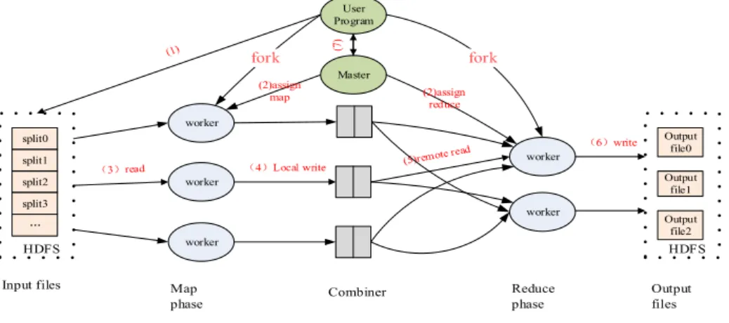
parallel environment. MapReduce operation is mainly composed with Map operation and Reduce operation. First() divides the metadata ﬁles into several chunks in accordance with(). Then the Master server distributes diﬀerent chunks to corresponding Worker servers for map. All the map operations are independent from each other and are highly parallel. They reads in the data in

the form of < Key, V alue >, and writes the intermediate results to the local ﬁle system in the

same form. Then the Master server adopts diﬀerent Worker servers for Reduce operation. This operation combines and output the intermediate results written by the map operation in the form of < Key, V alue > Input files split0 split1 split2 split3 … HDFS worker Map phase worker worker User Program Combiner worker worker Master (7 ) Output file0 Output file1 Output file2 HDFS （6）write Reduce phase Output files (2)assign map (2)assign reduce

Fig. 1: MapReduce model

2.2 Perceptron

A single-layer perceptron is a feed forward network which is equipped with a single-layer neuron and adopts the threshold to activate the function. By training the network weight, we can make the perceptron’s response to a group of input vectors to become the target output whose value is 0 or 1 and then classify the input vectors. Fig. 2 shows the model diagram of the single-layer perceptron neuron

p

1

p

₂

p

r

w

₁

w

₂

w

_r

Fig. 2: Model diagram of the single-layer perceptron neuron

As shown in Fig. 2, we take the weighted summation of the input components pi(i = 1,2,· · · ,r),

which is achieved with a weight component wi(i = 1,2,· · · ,r), as the input of the threshold

function. The adoption of the deviation b adds a new adjustable parameter to the network, and makes it much more easier for the network input to become the desired target vector.

(4)

2.2.1 Perceptron learning rule

Learning rule is an algorithm used for calculating the new weight matrix W and the new deviation B. It is adopted by perceptron to adjust the network weight so as to make the network’s response to the input vector to become the target input whose value is 0 or 1.

For the perceptron network whose input vector is P, output vector is A, and target vector is T, the parameter of the perceptron learning rule is adjusted in light of the conditions in which the output vector may possibly occur.

1. If the neuron output is correct, that is, a = t, then the neuron connective weight and the

deviation b will remain unchanged.

2. If the neuron output is 0, while the desired output is 1, that is, a = 0, t = 1, then the

algorithm for the modiﬁed weight is that the new weigh w i equals the former weight plus the

input vector p i.

3. If the neuron output is 1, while the desired output is 0, namely, a = 0, t = 1, then the

algorithm of the modiﬁed weight is that the new weight w i equals the former weightw i minus

the input vector p i.

In this paper, the deviationbis the weighted sum of the original setting value (a i) of the number

of objects in both the target cells and the neighbor cells in our outlier mining experiment. It varies with the weight, namely: b =

r

∑

i=1

ai×wi

According to the above analysis, the substance of the perceptron learning rule is that the weight variation equals either the negative or the positive input vector. Its speciﬁc algorithms are summarized as follows:

For alli, where i = 1,2,· · · , r, the formula of the modiﬁed weight for the perceptron is:

∆wi= (t−a)×pi (1)

And it can be represented with the vector matrix as:

W = W + EPT (2)

In Eq. (2), E is the error vector,

E = T−A (3)

2.3 K-means algorithm

K-means algorithm is one of the classic clustering algorithm whose main idea is clustering.The method ﬁrst randomly selects k objects as the initial averages or centers of the clusters, then calculates the distance between the rest data pointsand the centers, and then allocates those points to the clusters whose centers are the nearest; ﬁnally itcomputes the new averages of each cluster. The above process will be repeated until the criterion function converges to a given terminational threshold. Its pseudo-code algorithm is listed below:

Input: the number of clusters K, the dataset D which contains n objects

(5)

1. Randomly select K points from dataset D as the initial clustering center;

2. Calculate the distance between each point and the means(namely, the clustering centers); 3. Allocate each point to the cluster which is with the minimum distance;

4. Update the cluster means, namely, calculate each cluster mean again and take them as the new cluster centers;

5. Repeat Step(2) to Step(4), until the criterion function converges.

3 MR-ODCDC Algorithm

3.1 Related conceptions of MR-ODCDC

Deﬁnition 1: Distance-based outliers: An object O in a given dataset D is a distance-based

outlier which takes p and d as parameters and can be denoted as DB(p, d) outlier, if at least

fractionp of the objects in D lies greater than distance d from O.

Deﬁnition 2: Euclidean distance: For a given dataset D whose data dimension is d, the

formula of the Euclidean distance of the two data objectsO i and O j is deﬁned as:

dist (Oi,Oj) = v u u t∑d k=i (Oik−Ojk) 2 (4)

Deﬁnition 3: The ﬁrst layer neighbors ofCx,y, which is also called the immediately neighboring

cells of Cx,y, denoted as L1(Cx,y):

L1(Cx,y) ={Cu,v|u = x±1,v = y±1,Cu,v ̸= Cx,y} (5)

Deﬁnition 4: The second layer neighbors of Cx,y is of the thickness of two cells, denoted as

L2(Cx,y):

L2(Cx,y) = {Cu,v|u = x±3,v = y±3,Cu,v ̸= L1(Cx,y),Cu,v̸= Cx,y} (6)

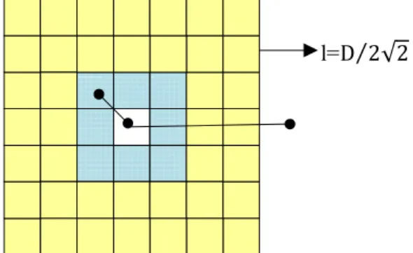
The data objects in the following two deﬁnitions are 2-D. If we partitioned each object into cells

whose length is l = D

2√2 suppose that Euclidean distance is adopted as the metric function for

measuring the distance between the objects, and letCx,y denotes the cell that is at the intersection

of rowxand column y, the conceptions and properties of the ﬁrst and the second layer neighbors

are as follows:

We can derive Definition 5 out from Definition 3 and Definition 4.

Deﬁnition 5: If Cu,v ̸= Cx,y, Cu,v is neither a layer 1 nor a layer 2 neighbor of Cx,y and for

objects pand q, p∈Cu,v,q∈Cx,y, then the distance between p and q must exceed D.

And since the combined thickness of L2(Cx,y) and L1(Cx,y) is the thickness of 3 cells, the

distance between p and q also exceeds 3l = 3D

2√2 > D.

Again from Deﬁnition 5, we can deduced another deﬁnition:

Deﬁnition 6: (1) If the number of the objects in Cx,y is more than M, that is, count>M,

(6)

both Cx,y and Cx,y is more than M, that is, count>M, none of the objects in Cx,y are outliers;

(3) If the summation of the number of the objects in Cx,y, L1(Cx,y) and Cx,y less than M, that

is, count<M, all the objects in are outliers.

l=D 2√2⁄

Fig.3: Cell structure chart Deﬁnition 7: The criterion function of K-means algorithm is:

E = k ∑ i=1 ∑ p∈KCi |p−m_i|2

Where E is the squared error summation of all the objects in the dataset; P is a point in the

space, representing a given object; and m_i is the average value of cluster KCi (both p and mi

are multidimensional). This criterion function increases the independence of the K generated

micro-clusters.

3.2 The basic idea of MR-ODCDC algorithm

The ideas of MR-ODCDC: The whole algorithm is divided into two subtasks by adopting a sequential combining MapReduce programming model. Each subtask is completed by using the MapReduce programming model in sequence. And the input of the second subtask is the output of the ﬁrst one.

The ﬁrst subtask: We ﬁrst cluster the dataset that is to be detected by employing K-means algorithm, then label all the points whose distance to the corresponding cluster centers are equal to or larger than the radius as the candidates of outliers. What calls for special attention is that if the number of the data points in a cluster is less than or equals to the pre-set number of outliers, the cluster can be directly labeled as a candidate set of outliers without comparing with the radius.

The second subtask: We detect among the newly generated candidates of outliers with the cell-based outlier detection algorithm. When compared with the traditional distance-based out-lier detection algorithms [11], our MapReduce-based outout-lier detection algorithm adopts both a single-layer perceptron and MapReduce, thus its performance is improved to some extent. Our algorithm ﬁrst trains the single-layer perceptron with a group of training data. Each group

of the data contains three elements, that is, the number of the objects in the target cell p 1.

The number of the objects in the layer1 neighboring cell p 2 and that of the second

(7)

N×(₄₉1 ×w1+₄₉8 ×w2+ 40₄₉×w3

)

. By training the perceptron, we get the optimal weight value and then can calculate the threshold.

MapReduce is adopted twice in the process of outlier mining. For the ﬁrst time, MapReduce is used to preprocess the original massive data. The Map operation obtains from the data objects in S the valid data items and maps each data object to the corresponding cell, then it outputs the key value of the data objects, the valid data items and the mapping information. For the second time, MapReduce is applied for outlier mining. In this process, the Map operation inputs the data blocks formed on the basis of mapping information, adopts the cell-based outlier detection algorithm which brings in weight to mine outliers and outputs the mining result. The Reduce operation integrates the results and outputs the outliers collection.

3.3 Description of MR-ODCDC algorithm

The ﬁrst subtask: the parallel algorithm of K-means method.

The MapReduce programming model adopts the idea of K-means algorithm. The Map

opera-tion randomly select k points as the initial clustering objects and each object is regarded as the

initial clustering means or centers. It then calculates the distance between the rest data points and those centers of the clusters and allocates each point to the corresponding cluster who has the shortest distance from it. The reduce operation calculates the mean of each cluster. The obove process will be repeated until the criterion function converges. If the adjacent clustering centers undergoes no change, the pseudo-code algorithm is as follows: Inputthe number of the points k, and the dataset D which contains n objects.

Output: corresponding collections of K clusters.

1. Randomly selectk points from datasetD as the initial central points and denote them asK.

2. While criterion function changes.

3. Compare the distances between the denoted data points and their corresponding central points with Map function, output the current data point and the number of its corresponding central point whose distance from it is the shortest.

4. Integrate the data points that are under the same central point with reduce function, calculate the new means and output the results as new central points.

5. End while.

The second subtask: cell-based outlier detection parallel algorithm.

The improved MapReduce-based outlier detection algorithm adopts a single-layer perceptron and MapReduce programming model. This algorithm can be further divided into two stages:

The ﬁrst stage: Map operation attains the valid data objects in S, maps each data object to

the corresponding cell and then outputs the key values of the data objects, the valid data items as well as the mapping information. The Reduce operation is responsible for the integration of the preprocessing results on the basis of the mapping information. It also outputs the integrative result. In this stage, MapReduce deals with the original massive data. The MapReduce-based outlier detection parallel algorithm ﬁrst trains the single-layer perceptron with a group of training data, and obtains the optimal weight value, then calculates the threshold with the value. The

training data consists of three elements which arethe number of the objects in the target cellp 1,

(8)

cell p 3. Deviation b is the product sum of the pre-set threshold and the weight, that is N× ( 1 49 ×w1 + 8 49×w2+ 40 49 ×w3 )

The second stage: Map operation inputs the data blocks formed in accordance with the map-ping information. It adopts the cell-based outlier detection algorithm in which weight value is introduced for outlier mining and outputs the mining results. Reduce operation integrates the mining results and outputs the collection of outliers. In this stage, MapReduce deals with outlier mining. The pseudo-code is listed below:

Input: Large dataset S, radius of neighborhood dmin, threshold of probability base η.

Output: Collection of abnormal objects.

(1) Prepare training data, train neuron network, attain weight value{w1,w2,w3}, calculate the

new threshold M = N×(₄₉1 ×w1+₄₉8 ×w2+ 40₄₉×w3

)

, where N is the number of the data inS.

(2) Randomly divide the large dataset S into several data blocks{S11,S12,· · · ,S1k}. Preprocess

each data block S1i through Map operation, map each data object to the corresponding cells and

attain S′_1i. Collect the preprocessed data blocks S′_1i with reduce operation, integrate the data

objects inaccordance with the mapping information and attain large dataset S 2.

(3) Divide the large dataset S 2 into several data blocks in light of the mapping information

{S21,S22,· · · ,S2k}. Mine the outliers by adopting Map operation:

fori= 1 to n //scan each cell Ci

if counti×w1 > M label the cell and the ﬁrst layer neighborhood cell as true (namely, none of

the points in the cell are outliers ) end for

for each unlabeled cell, do:

counti2= counti×w1+ w2

∑

j∈L1(Ci)

countj

if counti2> M, label this cell as true

else counti3= counti2+ w3

∑

k∈L2(Ci)

countk

if counti3≤M label this cell as false

else for each pointO in Ci

count0= counti2

scan each pointP in L2(Cj)

if dist (P,O)≤D:

count0 = count0+ 1×w3

(9)

if count0 > M, label point O as true

else label point O as false ( namely O is an outlier)

end if end for end if end if end for

The output of the second map operation are the collection of the outliers, or the results of the

< key, value > in the form of < dotmark, inf ormationof dotobject >, which also functions as the input of the second Reduce operation. Reduce operation carries out global statistics of all

received point information, and output the outliers in the form of< key, value > pair as the ﬁnal

result. The algorithm is accomplished when the Reduce operation is completed.

In this algorithm, the ﬁrst Map operation scans all the data objects, while the second Map operation ﬁrst scans and denotes all the cells, and then scans the objects in the undenoted or

unjudged cells. Thus, we can get the time complexity of the algorithm, namely O(ck_{+ n})_{, where}

k is the dimensionality of the dataset and c is a constant that based on the number of cells. In

our paper,k = 2, c is the number of cells of the data blocks input in each single Map operation,

and n is the number of the objects that are handled in a single Map operation. Therefore, both

candn in our algorithm are much smaller than those in the traditional algorithms, and the time

complexity of our method is thus accordingly reduced.

4 Analysis of Experiments and Results

4.1 Eﬃciency analysis

To verity the eﬀectiveness of our algorithm, we select 4 groups of hybrid datasets for experimental analysis from the UCI datasets [13], and then preprocess the selected datasets with the method [14] introduced. To make it more convenient for analysis and comparison, ﬁrst divides the original data into several types with a certain norm, then delete part of the objects from a certain type or several types of data to change the original datasets into imbalanced ones. The processed data information is shown in Table 1.

Table 1: Datasets description

dataset Number of samples Number of attributes category

Breast Cancer 699 10 2

Iris 150 4 3

Page block 5473 10 5

We evaluate the Outlier accuracy by comparing MR-ODCDC algorithm with MR-ODMD al-gorithm [15] and MR-AVF alal-gorithm [16]. Outlier accuracy, also known as outlier coverage which is introduced in [14], is very important metric for judging the validity of an algorithm. The ratio

(10)

of the true isolated points in the isolated points detected by an outlier detection algorithm to the original isolated points in the dataset is an important metric for evaluating the performance of the algorithm. A higher ratio indicates a better performance of the algorithm It is deﬁned as:

P=N

K

Where P is the accuracy, N is the number of the outliers detected by the algorithm, and K is

the number of the outliers in the dataset.

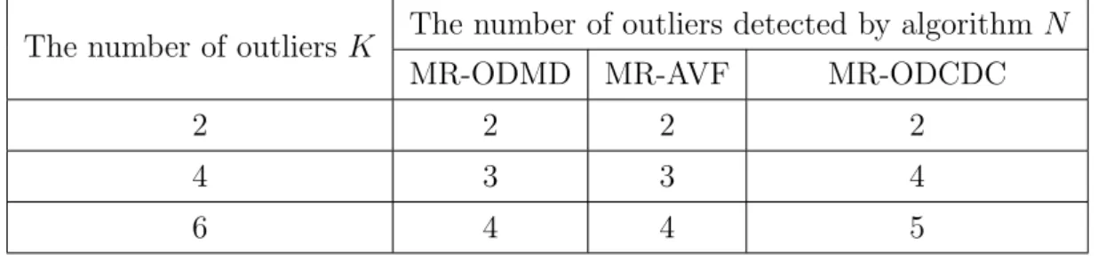
Table 2: Iris (6 outliers)

The number of outliersK The number of outliers detected by algorithm N

MR-ODMD MR-AVF MR-ODCDC

2 2 2 2

4 3 3 4

6 4 4 5

Table 3: Breast cancer (39 outliers)

4 4 4 4 8 6 7 7 16 13 14 14 24 19 21 22 32 29 28 30 39 32 32 34

Table 4: Page blocks (280 outliers)

50 28 30 35

100 45 42 55

200 79 84 92

250 110 105 140

280 119 125 160

From the above 3 tables, we can see that, our MR-ODCDC algorithm is of good precision. For 2-class outliers detection, taking Breast Cancer dataset as an example, the performance of our MR-ODCDC algorithm is slightly better than the other two algorithms. And for normal

(11)

multi-class outliers detection, such as outlier detection in Iris dataset and Page blocksdataset, our MR-ODCDC algorithm is much more eﬀective. This is because our algorithm successfully eliminates part of the normal data in the original dataset and reduces the number of the objects in the dataset by clustering the data objects with K-means algorithm, and meanwhile many more outliers are discovered, thus the precision of the ﬁnal result is greatly improved.

4.2 Analysis of parallel experiments and results

In our experiments, Hadoop cluster platform is set up on Ubuntu 12.04 with several PCs, JDK version is 1.7, and each node is formed with a PCwhose CPU is Intel Celeron(R) CPU E3500, master frequency is 2.70GHz, RAM is 2GB, and network card is 1 kilomega, we make one PC as the host node, denoted by Master (namely Na outlier detection meNode), which is responsible for schedule; and the others as work node, denoted by Slave (namely, DataNode), who calculate. In Hadoop cluster conﬁguration, the maximum loads of mapper are set by each node, the maximum

load Reducer (mapred. tasktracker. map | reduce. tasks. maximum) is set to 2, and the size of

distributed generation of the whole colony HDFS is 1.2TB.

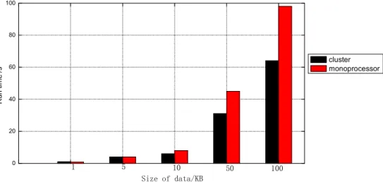
To prove that our algorithm can perform better in handling massive data, our experiment adopts the KDD CUP1999 dataset [17] as its experimental data. We can modify the dataset with software [18] and attain 5 datasets whose size are 1k, 5k, 10k, 50k, 100k, respectively. In the condition that 4 PCs are clustered, the computing time of each dataset are successively 2.142s, 4.356s, 7.019s, 35.502s, 65.487s. As shown in Fig. 4, when the size of the dataset is under 5k, there is little diﬀerence between the performance of cluster processing and uniprocessing. And the former even takes a longer time than the latter for the reason that the base time of MapReduce is rather long, most of which is taken by data sharping, generation of the sorting numbers of the intermediate ﬁles and the communication between the nodes. While the clustering performance of MapReduce will increase as the size of the dataset gradually grows larger from 10k to 100k. The run time of the clustering performance is improved by 33.54%, when compared with that of the uniprocessing. 0 20 40 60 80 100 R u n t im e / s cluster monoprocessor 1 5 10 50 100 Size of data/KB

Fig.4: Comparison of run time between cluster and monoprocessor

To better demonstrate the advantage of clustering processing, we use 1PC, 2PCs, 4PCs and 8 PCs to respectively detect the outliers in the datasets whose size are 1k, 5k, 10k, 50k, 100k. The

(12)

computing time are illustrated in Fig. 5. As shown in Fig. 5, when the size of the dataset is rather small, the computing time of the MapReduce-based algorithm is slightly higher than that of uniprocessing due to the base time taken by MapReduce operation. And still, as the size of the dataset gradually grows to 10k, the acceleration of uniprocessing continues to be larger than that of clustering processing. However, the larger the number of the DataNodes is, the stronger the computing power of our algorithm will have. When the size of the dataset reaches 100k, the eﬃciency of clustering processing improves by 54.13%, comparing with that of uniprocessing. And the clustering operation with 8PCs has the minimum speed-up ratio, thus it has the shortest run time. 0 10 20 30 40 50 60 70 80 90 100 R u n t im e / s 1 pc 2 pcs 4 pcs 8 pcs Size of data/KB 1 5 10 50 100

Fig.5: Comparison diagram of run time

5 Conclusion

Outlier detection is a branch of great importance in the field of data mining and it has already found wide application in many areas. The traditional distance-based outlier detection algorithms are belong to memory resident method, which is less than ideal in dealing with massive data. In this paper, we propose a two-stage outlier detection algorithm which is based on MapReduce programming model and adopts the K-means algorithm for clustering. Our algorithm first di-vides the dataset into several micro-cluster components on the basis of K-means algorithm ,then trains the single-layer perceptron with the training data in the micro-cluster components to at-tain the optimal weight; finally it further improves its efficiency by realizing parallelization with the MapReduce programming model. We have experimentally demonstrate that our algorithm for outlier detection has advantages over the existed distributed outlier detection algorithms on efficiency and accuracy in dealing with large high dimensional dataset. To further extend the ap-plicability of outlier detection techniques, in future, we will try to tackle several other challenging problems in this field, such as the outlier detection in uncertain data and that in complex data objects which includes spatial data, spatio-temporal data and multimedia data, etc.

(13)

References

[1] A. R. Xue, S. G. Ju, W. H. He, W. H. Chen, Research on Local Outliers Mining Algorithm. Chinese Journal of Computers, vol. 30, no. 8, pp. 1455-1463, 2007.

[2] J. W. Han, M. Kamber, Data Mining: Concepts and Techniques (2nd edition). Morgan Kaufmann Publishers, San Francisco, 2006.

[3] P. N. Tan, M. Steinbach, V. Kumar, Introduction to Data Mining, Addison-Wesley, New York 2006.

[4] C. P. Hu, X. L. Qin, ADensity-based Local Outlier Detecting Algorithm, Journal of ComputerRe-search and Development, vol. 47, no. 12, pp. 2110-2116, 2010.

[5] V. Barnet, T. LewisOutliers, Outliers in Statistical Data, John Wiley and Sons, New York, 1994. [6] T. Johnson, I. Kwok, Ng. Raymond, Fast Computation Of 2-dimensional Depth Contours, ACM

Internal Conference on Knowledge Discovery and Data Mining, New York, 1998.

[7] M. M. Breunig, H. P. Kriegel, Ng. Raymond, LOF: Identifying Density-based Local Outliers, ACM Internal Conference on Knowledge Discovery and Data Mining, New York, 2000.

[8] E. M. Knorr, Ng. Raymond, Algorithms for Mining Distance-based Outliers in Large Dataset, ACM Proceedings of the 24rd International Conference on Very Large Data Bases, New York 1998: 392-403.

[9] A. K. Jain, M. N. Murty, P. J. Flynn, Data Clustering: AReview, Journal ACM Computing Surveys, vol. 31, no. 3, pp. 264-323, 1999.

[10] K. Chen, W. M .Zheng, Cloud Computing: System Instances and Current Research, Journal of Software, vol. 50, no. 2, pp. 70-71, 2009.

[11] P. Mell, T. Grance, The NIST Deﬁnition Of Cloud Computing, National Institute of Standards and Technology, Gaithersburg, 2011.

[12] J. Zhang, Z. H. Sun, M. Yang, Fast Incremental Outlier Mining Algorithm Based On Grid and Capacity, Journal of Computer Research and Development, vol. 45, no. 5, pp. 823-830, 2011. [13] C. Blake, C. Merz, UCI machine learning repository, http://www.ics.uci.edu/mlearnMRepository.

html.

[14] C. C. Aggarwal, P. S. Yu, Outlier Detection For High Dimensional Data, Proceedings of ACM SIGMOD international conference on Management of data, 2001.

[15] Y. P. Guo, J. Y. Liang, X. W. Zhao, An Outlier Detection Algorithm for Mixed Data Based on MapReduce, Journal of Chinese Computer Systems, vol. 35, no. 9, 2014.

[16] A. Koufakou, J. Secretan, J. Reeder, Fast Parallel Outlier Detection for Categorical Datasets using MapReduce, International Joint Conference on Neural Networks, 2008.

[17] W. W. Ni, G. Chen, J. P. Lu, Y. J. Wu, Z. H. Sun, Weighted Subspace Outlier Detection Algorithm Based on Local Information Entropy, Computer Research and Development, vol. 8, no. 2, pp. 153-172, 2002.

[18] D. Cristofor, D. Simovici, Finding Median Partitions Using Information-Theoretical Genetic Al-gorithms, Journal of Universal Computer Science, vol. 8, no. 2, pp. 153-172, 2002.