The handle
http://hdl.handle.net/1887/85168
ho
lds various files of this Leiden University
dissertation.
Author:
De Paula Bueno, M.L.
Unraveling Temporal Processes using
Probabilistic Graphical Models
Cover background image: Davide Guglielmo Printed by Gildeprint
ISBN:9789464020519
IPA dissertation series: 2015-11
Typeset using LATEX
The work in this thesis has been carried out under the auspices of the research school IPA (Institute for Programming research and Algorithmics).
This work is part of the research programme Design and Analysis of Secure Dis-tributed Protocols (DASDiP), which is (partly) financed by the Netherlands Organi-sation for Scientific Research (NWO).
SIKS Dissertation Series No. 2020-02.
The research reported in this thesis has been carried out under the auspices of SIKS, the Dutch Research School for Information and Knowledge Systems. This thesis was supported by the Netherlands Organization for Scientific Research (NWO) as part of the “Careful” project (62001863), and by project “NORTE-01 -0145-FEDER-000016” (NanoSTIMA) financed by the North Portugal Regional
Operational Programme (NORTE2020), under the PORTUGAL2020Partnership
Unraveling Temporal Processes using
Probabilistic Graphical Models
Proefschrift
ter verkrijging van
de graad van Doctor aan de Universiteit Leiden, op gezag van Rector Magnificus prof.mr. C.J.J.M. Stolker,
volgens besluit van het College voor Promoties te verdedigen op dinsdag11februari2020
klokke15.00uur
door
m a r c o s l u i z d e pau l a b u e n o
Promotiecommissie: Prof. dr. T.H.W. Bäck (secretaris) Prof. dr. A. Plaat (voorzitter)
C O N T E N T S
1 i n t r o d u c t i o n 1
1.1 The relevance of temporal information . . . 1
1.2 Probabilistic graphical models . . . 2
1.3 Modeling sequential behaviors . . . 3
1.4 Adding more expressive power . . . 5
1.4.1 Time-dependent representation . . . 5
1.4.2 Factor-dependent representation . . . 5
1.4.3 Subprocess representation . . . 6
1.5 Thesis outline . . . 6
2 p r e l i m i na r i e s 9 2.1 Notation . . . 9
2.2 Bayesian networks . . . 10
2.2.1 Origin . . . 10
2.2.2 Representation . . . 10
2.3 Learning Bayesian networks . . . 13
2.3.1 Parameter learning . . . 13
2.3.2 Structure learning . . . 14
2.3.3 Decomposable scores . . . 16
2.4 Dynamic Bayesian networks . . . 17
2.4.1 Representation . . . 17
2.4.2 Learning . . . 18
2.5 Hidden Markov models . . . 19
2.5.1 Model architectures . . . 20
2.5.2 Families of HMMs . . . 21
2.5.3 Learning . . . 23
2.6 Learning with latent variables . . . 23
2.6.1 The expectation-maximization algorithm . . . 23
2.6.2 The Baum-Welch algorithm . . . 25
2.6.3 Number of latent states . . . 26
2.6.4 Structure learning with missing data . . . 27
3 a s y m m e t r i c h i d d e n m a r k ov m o d e l s 29 3.1 Introduction . . . 29
3.2 Basic notions . . . 30
3.3 Asymmetric hidden Markov models . . . 32
3.3.1 Model specification . . . 32
3.3.2 Parameterization . . . 33
3.3.3 Representation aspects . . . 35
3.4 Learning . . . 37
3.4.1 Learning setting . . . 37
3.4.2 Expectation step . . . 37
3.4.3 Maximization step . . . 38
3.5 Assessment via simulations . . . 41
3.5.1 Model selection . . . 41
3.5.2 Datasets . . . 42
3.5.3 Results for symmetric models . . . 42
3.5.4 Results for asymmetric models . . . 44
3.6 Experiments with real-world datasets . . . 48
3.6.1 Datasets . . . 48
3.6.2 Results . . . 50
3.6.3 Problem insight . . . 53
3.7 Related work . . . 55
3.8 Conclusions . . . 57
3.A Proofs . . . 58
4 p r e d i c t i n g d i s e a s e d y na m i c s: a c a s e s t u d y o f p s y c h o t i c d e p r e s s i o n 61 4.1 Introduction . . . 61
4.2 Related work . . . 62
4.3 A probabilistic framework for capturing disease dynamics . . . . 63
4.3.1 Latent variable modeling . . . 63
4.3.2 State trajectories . . . 64
4.3.3 Exploring medical outcomes . . . 65
4.3.4 Selecting states . . . 65
4.4 Data . . . 67
4.4.1 Patients . . . 67
4.4.2 Baseline and follow-up variables . . . 67
4.4.3 Depression assessment . . . 68
4.5 A model for psychotic depression . . . 68
4.5.1 General and intervention-specific model . . . 68
4.5.2 Model parameters and structure . . . 69
4.6 Results . . . 70
4.6.1 Model dimension . . . 70
4.6.2 Identified states . . . 71
4.6.3 Dynamics . . . 72
4.6.4 Comparing interventions . . . 72
4.6.5 Reachability trend per treatment . . . 73
4.6.6 Reachability trend per starting state . . . 73
4.7 Validation . . . 73
4.7.1 Model validation . . . 73
4.7.2 Outcome validation . . . 76
4.8 Conclusions . . . 76
c o n t e n t s vii
4.B Dynamics of intervention-specific models . . . 78
4.C Confidence intervals of reachability trend differences . . . 78
5 u n d e r s ta n d i n g m u lt i m o r b i d i t y t h r o u g h c l u s t e r s o f h i d -d e n s tat e s 81 5.1 Introduction . . . 81
5.2 Health-care event data . . . 83
5.2.1 Representation . . . 83
5.2.2 Modeling . . . 84
5.3 Identifying transition patterns . . . 84
5.3.1 Clusters of states . . . 84
5.3.2 Transition patterns . . . 84
5.4 Case study . . . 86
5.4.1 Variables and observations . . . 86
5.4.2 Sample . . . 87
5.4.3 Number of hidden states . . . 87
5.4.4 Clinical interpretation of clusters . . . 88
5.5 Experimental results . . . 89
5.5.1 Model dimension . . . 89
5.5.2 Clusters . . . 89
5.5.3 Transition patterns . . . 90
5.5.4 Clinical interpretation of clusters . . . 90
5.5.5 Are the clusters needed? A comparison to Markov chains 93 5.6 Related work . . . 94
5.7 Conclusions . . . 94
6 pa r t i t i o n e d d y na m i c b ay e s i a n n e t w o r k s 97 6.1 Introduction . . . 97
6.2 Related work . . . 99
6.3 Partitioned dynamic Bayesian networks . . . 100
6.3.1 Model specification . . . 100
6.3.2 A heuristic search procedure . . . 102
6.4 Empirical evaluation via simulations . . . 104
6.4.1 Simulation parameters . . . 104
6.4.2 Learning and evaluating PDBNs . . . 105
6.4.3 Results and discussion . . . 106
6.4.4 Small datasets . . . 108
6.5 Learning temporal models of psychotic depression . . . 110
6.5.1 Bayesian networks in psychiatry . . . 110
6.5.2 Problem description and data . . . 111
6.5.3 Heuristic learning . . . 112
6.5.4 Transition structures . . . 114
6.6 Model assessment from a clinical perspective . . . 114
6.6.1 Marginals of symptoms over time . . . 114
6.7 Conclusions . . . 120
7 e x c e p t i o na l m o d e l m i n i n g u s i n g d y na m i c b ay e s i a n n e t w o r k s123 7.1 Introduction . . . 123
7.1.1 Motivating example . . . 124
7.2 Related work . . . 125
7.3 Temporal exceptional model mining . . . 125
7.3.1 Temporal targets . . . 125
7.3.2 Subgroups . . . 126
7.3.3 Comparing subgroups . . . 128
7.3.4 Exceptional subgroups . . . 128
7.3.5 Problem statement . . . 129
7.4 Exceptional dynamic Bayesian networks . . . 129
7.4.1 Dynamic Bayesian networks . . . 129
7.4.2 Distance function . . . 130
7.4.3 Scoring function . . . 131
7.4.4 Exceptional subgroups . . . 131
7.5 Identifying exceptional subgroups . . . 132
7.5.1 Distribution of false discoveries . . . 132
7.5.2 Subgroup search . . . 132
7.5.3 Exceptionality test . . . 133
7.5.4 Search optimization . . . 134
7.6 Experiments with simulated data . . . 135
7.6.1 Data . . . 135
7.6.2 Evaluation . . . 135
7.6.3 Results . . . 136
7.6.4 Similar ground truth models . . . 137
7.6.5 Discussion . . . 138
7.7 Data of funding applications . . . 139
7.7.1 Data . . . 139
7.7.2 Discovered subgroups . . . 140
7.7.3 Validation . . . 140
7.8 Conclusions . . . 140
8 d i s c u s s i o n 143 8.1 Contributions . . . 143
8.1.1 Asymmetry in models . . . 143
8.1.2 Generation of hypotheses on processes . . . 144
8.1.3 Capturing hidden (non-observed) aspects of processes . . 144
8.1.4 Taking into account the size of datasets . . . 144
8.1.5 Temporal subgroups . . . 145
8.2 Future work . . . 145
8.2.1 Asymmetry in models . . . 145
8.2.2 Generation of hypotheses on processes . . . 145
c o n t e n t s ix
8.2.4 Taking into account the size of datasets . . . 146 8.2.5 Temporal subgroups . . . 147
b i b l i o g r a p h y 149
s u m m a r y 163
s a m e n vat t i n g 165
a c k n o w l e d g m e n t s 167
c u r r i c u l u m v i ta e 169
1
I N T R O D U C T I O N
1.1 t h e r e l e va n c e o f t e m p o r a l i n f o r m at i o n
The comprehension of real-world phenomena is often challenging, as their charac-terization might depend on some notion of time. A resulting lack of insight may stem from the fact that a single snapshot of a temporal process reveals only a part of its behavior, which may be insufficient for its complete understanding. This is the case, for example, when one contrasts a single instance of the observation of symptoms of a patient with a chronic disease against the longitudinal view of multiple instances of observations of symptoms: whereas the latter will offer a temporal view of the underlying disease process, the former will not shed any light upon disease dynamics.
In many everyday tasks, such as walking, cooking, sleeping and so on a role of temporal information can be identified. In professional fields, such as for example in psychiatry, the efficacy of pharmacological interventions in mental disorders only can be properly studied when the research is supported by collecting temporal data [3]. Such temporal information will tell for example how long it
takes before a treatment becomes effective and how long and how often a patient should take a particular drug. Also in many other diseases, in particular those with a chronic duration, temporal information is of paramount importance to gain insight into speed of progress or recovery.
Thus, given the importance of information about time in everyday and pro-fessional life, when one wishes to mathematically model processes of human artifacts, for example cyberphysical systems, or processes in the life sciences, usually time will be one of the parameters that need to be taken into account. It is not surprizing that predictions about the future are often more accurate when taking into account the history than when not relying on such information [63].
Of course, reasoning with time not only is concerned with predicting the future given the past, but can go in any other direction: from the present going back in time to understand the past, or from assumptions in the future going back in time to understand which past conditions are needed to make a particular future feasible. Whether these kinds of temporal reasoning are possible is determined by the nature and capabilities of the mathematical models and reasoning methods employed.
In this thesis, temporal processes are modeled as stochastic processes. Such processes typically involve one or more random variables that can be repeatedly observed. More importantly to their characterization, however, is that past observations have influence on future observations, which assigns to a temporal process a sequential nature. In other words, it is not just a matter of merely observing variables at different moments, or making repeated measurements of variables. On the other hand, by considering the sequential nature of such processes, additional challenges are introduced due to the increased modeling complexities that come along.
1.2 p r o b a b i l i s t i c g r a p h i c a l m o d e l s
An innate property of temporal processes is change, which renders them a stochastic nature. This makes probability theory a suitable tool for modeling such processes. Probabilistic models naturally take into account uncertainty, and can be used for multiple purposes: to predict the behavior of process variables in the future, discover associations between variables (e.g. which variables have more or less influence on a certain variable), and to pinpoint causes that could explain abnormal behavior.
Deriving models from data is a reality nowadays. This is because not only data storage technology has advanced (e.g. hardware capacity), but also more data is currently being generated, by means of sensor devices, content posted on the Internet, hospitals, health care services, etc. Obtaining statistical models from data which are expressive enough and can provide answers in reasonable running time is, however, not trivial. One major reason is that the process variables might interact in a very large number of ways. Without prior knowledge on the problem at hand, there is typically no obvious way as to how to reduce the space of models that might be of interest. In the past, researchers often relied on overly simplistic models (see e.g. [70]) to make model building feasible.
One solution to the parsimony problem faced by researchers is found with the adoption of probabilistic graphical models (PGMs, for short) [104,136]. PGMs
combine probabilities with graph theory for providing a graphical representa-tion of probability distriburepresenta-tions. With the representarepresenta-tion of PGMs it becomes much easier to represent statistical properties suitable for the problem at hand. Well-known PGMs include Bayesian networks, hidden Markov models, Markov random fields, among others. PGMs allow for a move from probability distri-butions, which are rich in detail, to graphs that abstract away from such details by encoding independence relationships. This occurs by means of aqualitative semantics entailed by the graphical structure of PGMs.
1.3 m o d e l i n g s e q u e n t i a l b e h av i o r s 3
demanding. PGMs also have a quantitativesemantics by assigning numerical parameters to nodes in the graph, which allows for computing probability queries with full detail.
When it comes to model building, a number of advantages result from using graphs to represent distribution properties. At the domain-expert level, it is possible to specify the desired level of restrictions on the way variables can interact probabilistically. For example, one might say that the variables should be independent (leading to an empty graph), or that interactions should follow a tree-like pattern, or even specify detailed interactions. The language of graphs is intuitive enough to allow one to easily specify such patterns. Independence relationships between variables can also be derived in a completely algorithmic manner without any expert knowledge, as methods have been developed for learning the graphical structure of PGMs from data [163,169]. A hybrid approach
is also possible by combining expert knowledge with data-driven learning.
1.3 m o d e l i n g s e q u e n t i a l b e h av i o r s
Dynamic Bayesian networks (DBNs, for short) [68,104,124] are well-known PGMs
used for representing temporal processes. The process that a DBN models is assumed to be a first-order process (or memoryless), which means that the future state of the process depends only the present state. The process is also assumed to be time homogeneous, which means that probabilities for transitioning from time t to time t+1 are the same for every t ≥ 0. As a result, DBNs offer a parsimonious representation of temporal processes by requiring the specification of typically a small number of probability parameters. DBNs can also be seen as extensions of discrete Markov chains to multiple variables. Example1.1discusses
the dynamics of a mental disorder treatment based on DBNs.
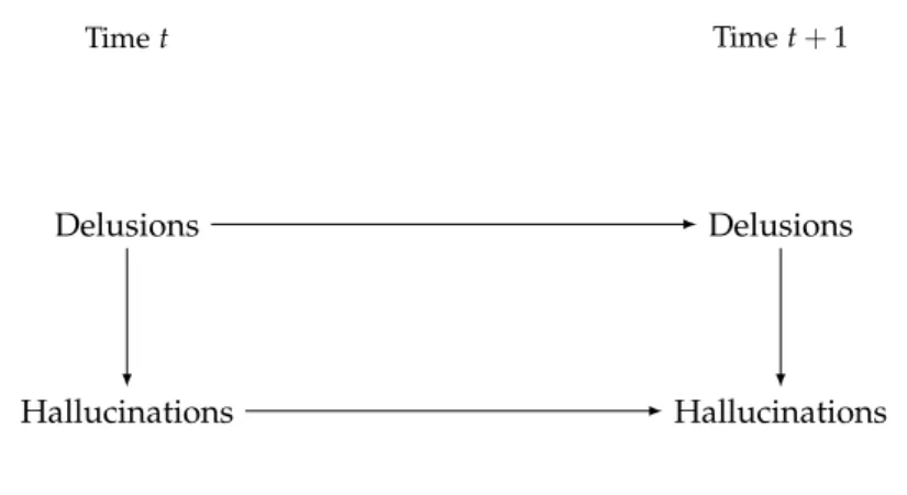
Example1.1.Suppose we want to model the symptom dynamics of patients with
psy-chotic depression [147], which is a depressive disorder with psychotic features. On a regular basis, two psychotic features (Delusions and Hallucinations) and Depression are measured for each patient. Due to the DBN assumptions aforementioned, the structure of a DBN for this problem is given by:
• A graph over the variables {Delusions, Hallucinations, Depression} indicating the symptom interactions at t=0.
• A graph over {Delusions(t),Hallucinations(t), Depression(t), Delusions(t+1), Hallucinations(t+1),Depression(t+1)}indicating the transitioning interaction of symptoms at two any time points, where t≥0.
Timet
Delusions
Depression Hallucinations
Timet+1
Delusions
Depression Hallucinations
Figure1.1: Transition structure of a dynamic Bayesian network that represents symptom interaction of psychotic depression patients.
In Figure1.1, an arc between two variables indicates that these variables may
be statistically dependent. On the other hand, two variables that are indirectly linked in the graph can still be statistically dependent, however this depends on the configuration of other variables in between them. When two variables are not linked directly nor indirectly, they are statistically independent [136].
Each arc of a DBN can refer to aninstantaneousinteraction, i.e. an interaction within the same time point, or a temporal interaction, i.e. an interaction that occurs at different time points [104]. The temporal arcs should satisfy the natural
temporal order, i.e., there must be no arcs with direction from future to past. In Example1.1, the instantaneous arc from Delusions to Hallucinations indicates
that at any point where measurements were made, delusions and hallucinations are statistically correlated. On the other hand, the temporal arcs for current depression to future depression means that the depression score of a patient at a certain week has influence on the patient’s depression the week after (as one would expect in general).
What makes the model of Figure1.1a temporal model is the temporal arcs,
because otherwise variables at a time pointt2would be statistically independent
of any variable at time t1 < t2. The instantaneous interactions are not strictly
needed for the model to be temporal, but they are often used to represent more complex statistical relationships.
As the process is assumed to be time homogeneous, in the model of Example
1.1not only the graphical structure is fixed over time, but also the numerical
1.4 a d d i n g m o r e e x p r e s s i v e p o w e r 5
1.4 a d d i n g m o r e e x p r e s s i v e p o w e r
One consequence of the compactness of models as DBNs is that they capture theaverageprocess behavior over time. This is because by having a transition model that is time invariant, the structure and numerical parameters of a DBN are the same for every time point. However, this might not always be desirable, because processes might change over time. By restraining ourselves to models that represent average behaviors, we might lose the opportunity to learn important insight about processes.
Process change might be captured by different ways. One would expect that real processes are in constant change. However, we would like to capture sensible process changes in our models, which would allow us to arrive at parsimonious explanations of the process at hand. We discuss3situations (orchallenges) where
it is desirable to represent processes in a more expressive way.
1.4.1 Time-dependent representation
One situation where we might be interested in more expressive models occurs when we wish to capture process change that manifests by varying variable interaction over time. For example, if the instantaneous and temporal interactions between Hallucinations and Depression are substantially different over time in Example1.1, one would likely obtain a better understanding of patient evolution
by modeling symptom interaction change in an explicit fashion.
In the case of models such as DBNs, process change could manifest as changes in the graphical structure, numerical parameters, or both. One challenge that arises in modeling is the identification of process change-points (or regime change) which take into account reasonable process change assumptions.
1.4.2 Factor-dependent representation
A different way of looking at process change is by identifying latent variables. Such factors can be seen as unmeasured quantities that are missing or difficult to be measured [178]. Latent variables can also be seen as categories or abstract
concepts derived from observable data, such as intelligence and extraversion in the context of human behavior [17]. In the latter case, latent variables might act
as a dimensionality reduction tool of observable data as it might be easier to understand the data in terms of the usually more compact latent representation. In Example1.1, latent factors that might be associated to process change could
be medical treatment, environmental factors (age, gender, climate, etc.), genetic expression, etc. Some of these factors might actually happen to be measured (e.g. medication and dosage), which would allow for explicitly including them as observable variables. At other times we are interested in learning latent concepts from observable data, such as patient clusters in Example1.1, which might help
Hidden Markov models (HMMs, for short) [138, 141] are PGMs that use
latent variables to model sequential processes. HMMs can capture very complex distributions by using a suitable latent state space [13]. The standard assumption
in HMMs is that observable variables are independent given the latent state. However, representing complex observed behavior based on such assumption can require too many states [76]. This is undesirable for several reasons, e.g.,
computing cost and less interpretable models.
Extensions of HMMs that are able to represent more general variable inter-action have been proposed [12, 76,102]. One challenge that arises is a better
understanding of how such HMMs compare in theory and in practice. Another relevant challenge is how to generate problem insight from more expressive HMMs which can help one understand the dynamics of processes (e.g. disease processes) in an effective way. This is relevant because the task of interpreting latent states is usually not straightforward.
1.4.3 Subprocess representation
A different viewpoint on process change concerns the identification ofsubprocesses which deviate considerably from the main model (or main process). We refer to ‘main process’ and ‘subprocess’ as processes associated to the model of the whole dataset and the model of a subset of the data respectively. In this situation, we would like to identify subsets of the data that are also representative enough, because it is easy to come up with very specific subprocesses made out of just a few data points (hence, not representative).
In Example1.1, there could exist a subset of patients with certain psychotic
symptoms that have a substantially slower response to treatment than the average patient response. We would like to identify such subsets (or subprocesses) in an automatic fashion. However, we cannot directly identify such subprocesses by models such as standard DBNs and HMMs.
One approach to identifying deviating subprocesses is the exceptional model mining (EMM, for short) [57,110], whose goal is the discovery of exceptional
models (in the sense of significantly different) associated to subsets of the data. However, EMM has been limited to either static data or univariate temporal data [112]. It would be desirable to extend the EMM framework for more general
temporal data.
1.5 t h e s i s o u t l i n e
This work addresses the discovery of structure from temporal data that can aid the comprehension of the underlying processes. For convenience, this work is divided into three parts as follows. In Chapters3-5, we investigate the underlying
structure of processes by means of models that use latent variables. In Chapter6,
1.5 t h e s i s o u t l i n e 7
how temporal data can be decomposed based on data subgroups that have a substantially different characterization in terms of a set of target variables compared to the distribution of those targets in the whole data. As a result, Chapter7provides a different characterization of process structure compared to
those of other chapters.
In order to demonstrate the usefulness of the proposed methods, we use real-world data from several domains, including medical data (e.g. primary care and clinical trials), industrial processes and business processes. We also discuss problem insight that can be obtained by the application of the methods to such datasets. We summarize the content of each chapter in the following.
c h a p t e r 2: Preliminaries, where notions on PGMs relevant for representing
temporal processes are discussed.
c h a p t e r 3: Asymmetric hidden Markov models, where we introduce the family
ofasymmetric hidden Markov models(HMM-As, for short) for representing local structure of distributions in the hidden Markov model framework. An algorithm for learning HMM-As from temporal data is proposed. HMM-As are empirically evaluated based on simulated data and real-world data from several domains. This chapter is based on the publications [25] and [23]. c h a p t e r 4: Predicting disease dynamics: a case study of psychotic depression, in
which a methodology is proposed for aiding the generation of medical hypotheses based on structured hidden Markov models learned from data. The methodology is used to uncover insight on the dynamics of different pharmacological therapies undertaken by psychotic depression patients. This chapter is based on the publications [27] and [28].
c h a p t e r 5: Understanding multimorbidity through clusters of hidden states, where
we analyze the problem of disease interaction and multimorbidity in terms of patterns of transitions between latent states. We consider a study case of patients with disorders related to atherosclerosis based on a large primary care data, and show that multiple patient characterization can be associated to cluster of states. This chapter is based on the publication [26].
c h a p t e r 6: Partitioned dynamic Bayesian networks, in which we propose
parti-tioned dynamic Bayesian networks(PDBNs, for short) for representing tem-poral processes by means of a collection of dynamic Bayesian networks. We propose a learning algorithm for PDBNs which adds process cut-offs in a parsimonious way. PDBNs are evaluated experimentally based on simulations and real data. This chapter is based on the publication [24]. c h a p t e r 7: Exceptional model mining using dynamic Bayesian networks, where we
Subgroups are characterized by dynamic Bayesian networks. This chapter is based on the paper [22], which was submitted for publication.
c h a p t e r 8: Discussion, in which the results achieved in this work are
2
P R E L I M I N A R I E S
In this chapter, we fix the notation used throughout this work and present definitions on probabilistic graphical models that are relevant for the following chapters. We start off by covering the basics of Bayesian networks, then move to dynamic Bayesian networks and hidden Markov models, which extend the framework of Bayesian networks for handling temporal problems. Learning models from data is also discussed.
2.1 n o tat i o n
We first introduce the notation and a few conventions used throughout this work. In probability theory,random variablesare typically denoted by upper case letters, such asX, while thedomainof a random variableXis represented by dom(X), which represents the set of values thatXtakes on [52]. Adiscrete random variable
is a random variable which has a finite or countably infinite domain, while a continuous random variablehas as domain a subset of the real numbers. A random variable is associated to a probability distribution, which assigns a probability value to each value of its domain (for discrete variables) or to real intervals of its domain (for continuous variables).
The probability distribution of a discrete random variableXwill be denoted by P(X), and the probability of a certain value x ∈ dom(X) will be denoted by P(X = x) or simply P(x) when no confusion can arise. The probability distribution of a continuous random variableYwith probability density function f(Y)is denoted byp(Y), and the probability thatYtakes values on a real interval [y1,y2]is indicated asp(y1≤Y≤y2). A set of random variables will be denoted
by a bold face letter, e.g.,X={X1, . . . ,Xn}. A probability distribution assigned
to a single random variable as inP(X)is called aunivariatedistribution, while the joint distribution assigned to set of variables{X1, . . . ,Xn}is called amultivariate
distribution and is denoted byP(X1, . . . ,Xn)orP(X).
Intemporal modeling, each variable is often measured repeatedly, such that a variableXat timetwill be referred to asX(t). This means that the domains of X(t), for allt≥0, are the same. For the discrete time points{t
1, . . . ,t2}, where
t2 ≥ t1 ≥ 0, the notation X(t1:t2) will be used to refer to the set of variables {X(t1), . . . ,X(t2)}.
2.2 b ay e s i a n n e t w o r k s 2.2.1 Origin
A Bayesian network (BN, for short) is a graphical model of a multivariate proba-bility distribution with independence constraints. Bayesian networks date back to the1980s [97,104,136]; their goal was to overcome the limitations of rule-based
expert systems from the previous decade that incorporated uncertainty in the form of numbers that had some resemblance to probabilities [115]. One important
limitation of such AI systems was the need for representing an unrealistic number of probabilities to perform probabilistic inference, a problem which was dealt with by making many simplifying assumptions. While this led to a substantial reduction in the needed number of probabilistic parameters, it also gave rise to poor performance in solving real-world problems, for example in medical diag-nosis [70]. By marrying probability theory with graph theory, Bayesian networks
allowed to provide the right balance in the number of probabilistic parameters needed to realistically represent the problem domain at hand.
A Bayesian network is a two-fold representation, as it encodes both qualitative and quantitative information about probability distributions. The qualitative side of a Bayesian network is given by a graph, whose semantics is associated to statistical independence statements. The quantitative side regards numerical probabilities, which are specified following the structure of the graph. As a result, BNs provide a compact, yet expressive way of representing probability distributions.
2.2.2 Representation
To define Bayesian networks over a set of random variables of interest, a few definitions are introduced first. AgraphG is a pairG= (V,A), whereVis a set of objectsi∈ {1, . . . ,n},n =|V|, callednodes, and A⊆V×Vis a set of node pairs callededges. IfG is adirected graph, then each edge ofAis an ordered pair (i,j), also represented byi →j, such that (j,i)6∈A. The edges are then called directed edgesorarcs. Ifi→j∈Ais an arc, theniis called theparentof nodej, andjis called thechildof nodei. If there is a directed path from nodeito nodej, theniis called theancestorofj, whereasjis called thedescendantofi.
IfGis anundirected graph, then its edges are unordered pairs, i.e., if(i,j)∈A
then also (j,i) ∈ A, simply represented as a set{i,j}. A directed acyclic graph (DAG, for short) is a directed graph with no cycles, i.e., there is no sequence of arcs of the form i → j → · · · → i (first and last node in the sequence are the same). As usual, each nodeiin the DAG withV={1, . . . ,n}will be associated in a one-to-one way to a random variableXifrom the set of variablesX1, . . . ,Xn
for the convenience of defining a Bayesian network. In the following, we shall refer to nodes and variables interchangeably and useXito refer to both the node
2.2 b ay e s i a n n e t w o r k s 11
One way to define Bayesian networks is from the notion of factorizing a joint probability distribution according to the structure of a graph as follows.
Definition2.1(Factorization).LetG= (V,A)be a directed acyclic graph with nodes
V={X1, . . . ,Xn}. A joint probability distribution P over the same variables factorizes
according toG if P can be written as:
P(X) =P(X1, . . . ,Xn) = n
∏
i=1
P(Xi|π(Xi)) (2.1)
whereπ(Xi)refers to the parents of the node XiinG, and each factor P(Xi|π(Xi))is
called a conditional probability table (CPT, for short).
Definition2.2(Bayesian network).A Bayesian network is a pairB = (G,P), where
P is a joint probability distribution that factorizes according to a directed acyclic graphG. The joint probability distribution P associated with a Bayesian network G
encodes conditional independences, if it holds for three mutually disjoint sets of variablesU,W,Z⊆Xthat ifP(U|W,Z) =P(U|Z)for any set of values of the variables inU,W,Z. It is said that the variables UandWareconditionally independent(underP) givenZ, written asU⊥⊥PW|Z. The set of all conditional
independent triplets associated to a joint probability distributionPis sometimes defined as I(P) ={(U,W,Z)|U⊥⊥PW|Z}.
The Bayesian network graph encodes independence relationships, which can be read off by means of a graphical property calledd-separation(directed separation) [136]. The notion of d-separation defines potential probabilistic influence between
variables based on the structure of the BN graph. This can be described by means of the notion of active trail [104]. A sequence of nodesσ = X1, . . . ,Xm in the
graphG is atrailif eitherXi →Xi+1or Xi ←Xi+1is an arc inG on the trailσ,
i = 1, . . . ,m−1, i.e., the direction of the arcs is ignored and only the fact that X1is connected by the trail toXmis taken into account. Now the trail between
X1 and Xm is called activeif for any Y on the trail σ, the connections of the
neighboring nodesUandW have the following directions:
• U←Y→W(divergent connection),U→Y →W (serial connection), or U←Y←W(serial connection), andYhasnotbeen observed, or
• U→Y←W(convergent connection orv-structure), whereasYor any of its descendants have been observed.
If a trail is not active, it is calledinactive.
Now consider the following three mutually disjoint sets of nodesU,W,Z⊆V. If all trails between any node inUand any node inWare inactive given (possibly empty) observations inZ, it is said that the set of nodesZd-separatesthe set of nodesUandW, written as
U⊥⊥dG W|Z
For the graphG we can now collect all d-separation triplets: I(G) ={(U,W,Z)|U⊥⊥d
The above definition can be used to provide a semantics of the BN graph in terms of independence statements that are entailed by the graph. For Bayesian networksB= (G,P)where the distributionPfactorizes according to the DAGG, it holds that I(G)⊆ I(P)[136]. This means that every independence that holds
in the BN graph must hold in the distribution. This explains why the interpreta-tion of d-separainterpreta-tion as condiinterpreta-tional independence is meaningful. However, the semantics makes also clear that the two independence relations I(P)and I(G) may not coincide.
Because of d-separation, the network structure of a Bayesian network can be seen as its qualitative part, while the quantitative part corresponds to the probabilities encoded in the CPTs. A Bayesian network example is provided in Example2.1.
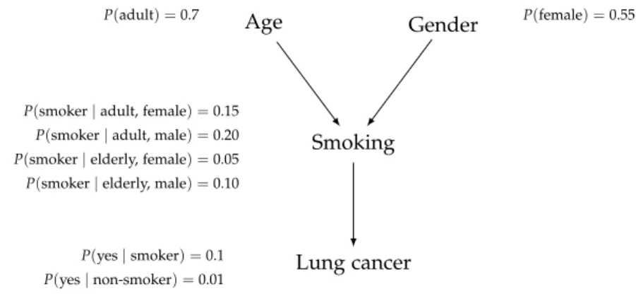
Example2.1.Assume we are interested in diagnosing lung cancer, as represented by
the variable C with dom(C) ={no, yes}. Other variables of interest are smoking (S), gender (G), and age (A), where dom(S) = {no, yes}, dom(G) ={female, male}and dom(A) = {adult, elderly}. Figure2.1shows the graphical structure and the CPTs associated to this Bayesian network. Independence relationships can be deduced from the graphical structure, e.g., having knowledge about smoking will make age and gender irrelevant for the prediction of lung cancer.
Age
P(adult) =0.7
Gender P(female) =0.55
Smoking
P(smoker|adult, female) =0.15 P(smoker|adult, male) =0.20 P(smoker|elderly, female) =0.05 P(smoker|elderly, male) =0.10
Lung cancer
P(yes|smoker) =0.1 P(yes|non-smoker) =0.01
Figure2.1: Bayesian network of the lung cancer example. Note that the structure and the CPTs in this example are fictional.
One advantage of the BN framework is that in the network structure one typically captures only the essential variable interactions, which often results in a substantial reductions in the needed number of probabilities to be specified. The BN of Example 2.1requires 1+1+4+2 = 8 independent parameters,
2.3 l e a r n i n g b ay e s i a n n e t w o r k s 13
The first step to using the BN representation is usually finding a suitable network structure for the problem at hand. One way to construct such a network structure is by manually defining the interactions among the involved variables that are supposed to hold in the domain, based on prior background knowledge and supported by domain experts. In that case, it is usually easier to think of interactions in terms of cause-effect relationships [47], although the semantics
of a Bayesian network per se does not embody a causality notion. The network structure can also be obtained from data. In any case, once the network structure is obtained, the parameters of the network nodes need to be estimated, which can also be done manually [71] or algorithmically [47].
2.3 l e a r n i n g b ay e s i a n n e t w o r k s
In practical situations, prior knowledge about the problem at hand might not be available for handcrafting a Bayesian network for the domain, for example, if it is too expensive to be obtained, nonexistent, or is prone to be incorrect. This motivates the need for Bayesian network learning algorithms [44,85,169], whose
goal is to automatically find a Bayesian network that suitably represents the distribution associated to the data. Bayesian network learning involves two steps: learning a network structure and learning numerical parameters. Handling each task also depends whether the data is complete or incomplete. In this section, we consider the case of complete data.
2.3.1 Parameter learning
In the parameter learning task, we assume the network structure is known. The goal is to estimate the CPTs of all the variables, i.e. the distributionsP(xi|π(xi))
for everyxi. Let us denote byθthe set of parameters associated to the Bayesian
network which are to be estimated, and letDbe a set of data pointsx[1], . . . ,x[m] of the formx[j] ={x1[j], . . . ,xn[j]}, wherexi[j]refers to the value of the variable
Xi taken in the jth data point. Each Xi is assumed to follow a categorical
distribution taking values on dom(Xi). We further assume that all data points of
Dare independent and identically distributed (i.e., i.i.d. samples). The likelihood function of the Bayesian network with structureG parameterized byθgiven the
dataDcorresponds to the probability ofDunder such model and is given by:
L(θ:D) =P(x[1], . . . ,x[m]: θ) (2.2)
=
m
∏
j=1
From the factorization of Bayesian networks we obtain:
L(θ:D) =
m
∏
j=1 n
∏
i=1
P(xi[j]|π(xi)[j]:θ) (2.4)
=
n
∏
i=1
P(xi[1]|π(xi)[1]:θ). . .P(xi[j]|π(xi)[j]:θ) (2.5)
Equation2.5shows that the likelihood function can be decomposed into a product
of independent terms, one for each node of the network structure. If we denote byθirk the parameterP(Xi=xk |π(Xi) =xr), then the likelihood function can
be further expanded as follows:
L(θ:D) =
n
∏
i=1x
∏
k,xrθirkNirk (2.6)
where Nirk is the number of times the configuration(Xi = xk,π(Xi) = xr) is
seen in D. The goal now is to find the set of parametersθthat maximize this
function, an approach known asmaximum likelihood estimation(MLE, for short). The parameters that maximize the likelihood function are denoted by ˆθ. It is
usually easier to work with the logarithm of Equation2.6, which is referred to as
the log-likelihood of the data. It is possible to show [104] that the maximization
of the log-likelihood leads to closed-form formulas for parameter learning as follows:
ˆ
θirk = Nirk
Nir (
2.7)
where Nir is the number of times the configuration(π(Xi) = xr) occurs inD.
These quantities are known assufficient statistics, and convey the idea that each parameter corresponds to the node’s proportional counts with respect to its parents. Once the optimal parameters ˆθare computed, the likelihood computed
based on ˆθis denoted by ˆL.
2.3.2 Structure learning
When the network structure is unknown, one resorts to learning the network structure from data. The goal of structure learning is to recover the structure of the hypothetical joint probability distribution underlying the data [50]. With
structure learning, one is able to discover the dependence structure of the domain, which can yield insight about qualitative influences that hold in the domain, both direct and indirect. Network structure learning is also important to make the parameter estimation in Bayesian networks feasible, although the structure should not be overly simplistic, otherwise relevant correlations might be missed.
The problem of structure learning can be formulated as an optimization prob-lem [7,42], also known asscore-basedapproach, whose goal is to find the network
structure ˆG that optimizes a scoring function: ˆ
G =arg max
G∈GScore(G,D) (
2.3 l e a r n i n g b ay e s i a n n e t w o r k s 15
whereGis the space of network structures, i.e. the set of directed acyclic graphs with nodes{X1, . . . ,Xn}. In general, finding optimal Bayesian networks has been
shown intractable [42,43]. Network structures can also be learned by means of the
constraint-basedapproach [118,136], which determines a network structure that is
consistent with the independence relationships that hold on the data. In the case of constraint-based learning, the worst case requires an exponential number of tests [118]. In the remainder of this chapter, we consider the score-based approach
and further elaborate on it.
Scoring functions for structure learning play a central role in this task and the literature offers a variety of them. One of the simplest score functions is the likelihood score [104], which indicates the probability of the data given the
model and was defined in Equation2.2. In the situation of unknown structure,
the likelihood score seeks the model (i.e. graph and parameters) that maximizes the likelihood:
maxL(G,θG:D) =max
G
max
θG∈ΘL
(G,θG: D)
(2.9)
=max
G
L(G, ˆθG: D) (2.10)
where Θ is the space of CPTs with regard to the graph G. Hence, in order to maximize the likelihood, one needs to find the structure ˆG that maximizes Equation 2.10, where each candidate structure has parameters fitted via MLE.
However, as the goal with model learning is to capture the true distribution of the data, using the likelihood score typically has severe limitations as follows. By adding more arcs to the network, the likelihood score never decreases and instead tends to increase [104]. Hence, by completely fitting to the data, one is
also fitting to the noise on the data, and the resulting network tends to be a fully connected graph. This usually leads to the problem of model overfitting, which means that the model does not generalize well (i.e. it performs poorly on new data).
One alternative score function is the Bayesian score, which adopts a Bayesian approach to modeling the structure and parameters that are to be estimated. In the Bayesian approach, one defines a structure priorP(G)and a parameter prior P(θG | G)for the possible ways a given structure can be parameterized. For a
candidate graphG, we can apply Bayes’ rule to obtain:
P(G |D)∝P(D| G)P(G) (2.11)
where the denominator P(D) can be dropped because it is the same for all the graphs. The Bayesian score is then defined by taking the logarithm of the right-hand side of Equation2.11:
In the priorP(G)one can model a prior distribution that might favor, e.g., sparser graphs. The termP(D| G)is known as marginal likelihood as it can be written as:
P(D| G) = Z
θG∈Θ
P(D|θG,G)P(θG | G)dθG (2.13)
Intuitively, the marginal likelihood weights the likelihood of the dataP(D|θG,G)
by different ways of selecting the parameters given the networkG. Hence, the marginal likelihood can be seen as an average of the likelihoods for the structure
G, as opposed to the maximum likelihood score, which looks only at the score that maximizes the termP(D|θG,G). The Bayesian score tends to favor simpler
structures if little data is available for learning [104], which provides a mechanism
to combat overfitting. By using Dirichlet priors on all parameters of the network, it is possible to show [104] that an approximation of the Bayesian score results
in the so-called Bayesian information criterion (BIC, for short), which is given as follows:
BIC(G |D) =−2·logL(θˆG: D) +K·logm (2.14)
whereKis the number of parameters of the network structureG, andmis the size of the dataset.
The goal now is to find the structureGthat minimizes the BIC score, where the termK·logmin Equation2.14acts as a penalty term. Equation2.14suggests that
the problem of structure learning can be seen as a model selection problem [182],
where one wishes to find the network structure that balances goodness-of-fit (the likelihood term) and model size. The scoring function is then coupled to a search procedure, which is often a heuristic procedure such as tabu search [77],
hill climbing, simulated annealing, among others [152], resulting in sub-optimal
network structures obtained in feasible running time.
Although heuristic procedures are often used in BN structure learning, re-search has shown that optimal structure learning can be done efficiently in some situations [31, 158]. Some techniques are able to scale to problems with
hun-dreds variables [50]. Research has also shown that it is possible to predict which
algorithms would be more suitable for optimal learning of a given instance [116].
2.3.3 Decomposable scores
In structure learning, a key computational property is that of decomposability. A score is decomposable if it is defined locally per node [50]. This allows for the
score of a candidate Bayesian networkB, also referred to as itsglobal score, to be given as a sum oflocal scores, one for each variable:
Score(B) =
∑
Xi∈X
Score(Xi,πB(Xi)) (2.15)
whereπB(Xi)refers to the parents ofXi inB. Decomposable scores allow for the
2.4 d y na m i c b ay e s i a n n e t w o r k s 17
addition, as such operations affect only the associated local scores. As a result, by exploiting this property, structure learning algorithms can scale reasonably well. Many scores commonly used in structure learning are decomposable, where the BIC is one such score [50].
2.4 d y na m i c b ay e s i a n n e t w o r k s
In this section we discuss extensions of Bayesian networks for modeling temporal processes by means of dynamic Bayesian networks (DBNs, for short). Learning DBNs from data is also discussed.
2.4.1 Representation
Dynamic Bayesian networks [68,124] extend Bayesian networks for modeling
tem-poral processes where uncertainty plays an important role. We restrain ourselves to dynamic systems in which all the variables of a setX={X1, . . . ,Xn}are
mea-sured together and repeatedly over time, which is represented byX(0),X(1), . . .. Further, the time interval between two measurementsX(t) andX(t+1), for any t≥0, is assumed fixed. This means that in such dynamic systems the sequential behavior of the involved variables is abstracted from the absolute time of their measurement.
In order to keep the model compact, a few additional assumptions about the process involved in the generation of Xare often considered [104], which we
describe as follows.
Definition2.3(Markovian dynamic system).A dynamic system over the variablesX
is first-order Markovian (or simply Markovian) if, for all t≥0,
P(X(t+1)|X(0:t)) =P(X(t+1)|X(t)) (2.16)
The Markovian assumption means that predicting the future state of the process depends only on its current state and not on previous states it has assumed. In this case, the process is also said to bememoryless. Another useful property is given as follows.
Definition2.4(Time-homogeneous dynamic system).A dynamic system over the
variablesXis time homogeneous (or time invariant) if P(X(t+1) |X(t))is the same for every t≥0.
Dynamic Bayesian networks provide a representation for Markovian time-homogeneous dynamic systems grounded on graphical models as defined next.
Definition2.5(Dynamic Bayesian network).A dynamic Bayesian network is a
Marko-vian time-homogeneous system(B0,B→)overX, where:
• B→ = (G→,P→)is a Bayesian network over the variables{X(t),X(t+1)}called
transition network. The variables ofX(t)have no parents in the transition network.
The transition network can also be seen as aconditional Bayesian network[104],
because it suffices to define the distribution P(X(t+1) | X(t))for defining this network. Although DBNs can be defined as semi-infinite systems [68], in practice
one reasons with a finite horizon{0, . . . ,T}. In this case, the DBN is unrolled so that a joint distribution over the process duration is specified as follows: the structure and parameters of all the nodes at time t = 0 come from the initial model, while the structure and parameters for any nodeX(it), wheret>0, come from the transition model.
From the previous definitions and assumptions, the joint distribution of a DBN over a time horizon{0, . . . ,T}is as follows:
P(X(0:T)) =P(X(0))
T−1
∏
t=0
P(X(t+1)|X(t)) (2.17)
=
n
∏
i=1
P0(X(i0)|π(X
(0)
i )) T−1
∏
t=0 n
∏
i=1
P→(Xi(t+1)|π(X
(t+1)
i )) (2.18)
where in Equation2.18it is shown that the joint can be written in a modular way
based on the factorization provided by the distributionsP0andP→. An example
of DBN for a medical problem is described in Example2.2.
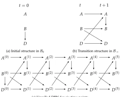
Example2.2.In a disease process, two symptoms (denoted by A and B) and the
adminis-tered drug quantity (denoted by D) are observed at regular time intervals for each patient. A DBN is used to model patient evolution, where the structure of the initial modelB0
and the transition modelB→are shown at the top of Figure2.2. FromB0andB→, an
unrolled DBN over six time points can be obtained, as shown at the bottom of Figure2.2.
In the transition model of a DBN the set of arcs from a variable at timetto a variable at timet+1 are often calledintra-temporalarcs, e.g., the arcsB(0)→D(0) andA(1)→B(1)in Example2.2. On the other hand, arcs between variables from
the same time point are calledinter-temporalarcs, such as A(0) → A(1)in this example.
2.4.2 Learning
Learning DBNs is to a considerable extent similar to learning (static) Bayesian networks. Let us consider a training setDofmi.i.d. sequences, where thejth sequence has observations of the formx[j](0), . . . ,x[j](mj). For convenience, we
denote byD0the initial slices ofD, which amount tomobservations, whereas we
denote byD→the transition instances ofD, which amount tom0 observations, where m0 = ∑m
i=1mi. The initial model B0 and the transition model B→ are
2.5 h i d d e n m a r k ov m o d e l s 19
t=0 A
B
D
(a) Initial structure inB0
t+1
A
B
D
t+1 A
B
D
(b) Transition structure inB→
A(0)
B(0)
D(0)
A(1)
B(1)
D(1)
A(2)
B(2)
D(2)
A(3)
B(3)
D(3)
A(4)
B(4)
D(4)
A(5)
B(5)
D(5)
(c) Unrolled DBN for six time points.
Figure2.2: An example of DBN for a disease process. The CPTs ofB0 andB→ are not shown.
In an MLE approach, by a similar reasoning as done with static Bayesian networks (Section2.3.1) it can be shown [68] that the BIC of a DBN(B0,B
→)with
structureG = (G0,G→)is given by:
BIC(G:D) =BIC0+BIC→ (2.19)
where
BIC0=−2·logL(θˆG0: D0) +K0·logm (2.20)
and
BIC→=−2·logL(θˆG
→:D→) +K→·logm0 (2.21)
such thatK0andK→denote the number of parameters of the initial and transition
models respectively.
Equation2.21in fact uses the conditional log-likelihood of the transition
in-stances, which is given by logL(θˆG→:D→) =∑mj=1∑tlogP(x[j](t+1)|x[j](t)). By
maximizing the BIC of B0 and the BIC of B→ independently, the BIC of the
complete DBN is maximized as well.
2.5 h i d d e n m a r k ov m o d e l s
quantities [178]. This might provide improved understanding of the problem at
hand, along with other potential advantages such as simplified model structure [67] and better model fit [179].
In this section, we discuss hidden Markov models (HMMs, for short), which can be seen as instances of DBNs from a representation perspective. We focus on several representation aspects of HMMs, while learning is covered in the next section.
2.5.1 Model architectures
In a general problem setting, we denote byX={X1, . . . ,Xn}the set of observable
features, and we assume that there is a set of state variablesS = {S1, . . . ,S`}
that we do not observe and are involved in the generation of Xover time. In such problem, we are interested in a temporal model that can be constructed and used feasibly, yet is realistic and insightful. To this end, different sets of assumptions are very often used, taking also into account domain characteristics. As a consequence, the variety of existing HMMs renders different probabilistic in-teractions betweenXandS(by interaction we refer to unconditional probabilistic dependence).
A general HMM framework is illustrated in Figure2.3[25], where the exact
form of interactions within states and within observables is abstracted. We start by defining the HMM which captures the interactions denoted by solid lines in Figure2.3and can be seen as a basis for several other HMMs.
time
hidden variables
observables higher-order
interactions
states-observables interactions
autoregressions
t−1 t
S1, . . . ,Sl
X1, . . . ,Xn
S1, . . . ,Sl
X1, . . . ,Xn
. . .
. . .
. . .
. . . t−2, . . . , 0
t−2, . . . , 0
t−2, . . . , 0
Figure2.3: An abstracted general HMM with hidden variables{S1, . . . ,S`}and observ-ables{X1, . . . ,Xn}. Solid arcs indicate interactions present in the independent
HMM and related models.
Definition2.6 (Hidden Markov model).A hidden Markov model is a Markovian
2.5 h i d d e n m a r k ov m o d e l s 21
• A=P(S(t+1)|S(t))is the transition distribution • B=P(X(t)|S(t))is the emission distribution
• υ=P(S(0))is the initial state distribution
and dom(S) ={s1, . . . ,sk}is called the state space of the model.
The above definition is based on those of dynamic systems given in Section2.4,
except that in an HMM we repeatedly measure not only observablesX, but also a latent variableS. In this case, there is a single latent variable per time point, hence
S={S}. It is customary to viewAas a matrix[aij],Bas a set{bj(k)}sj∈dom(S),
andυas a vector[υ(si)], where:
aij=P(S(t+1)=sj|S(t)=si) (2.22)
bj(k) =P(X(t)=xk|S(t)=sj) (2.23)
υ(i) =P(S(0)=si) (2.24)
The above notation will be useful when describing HMM learning (see Section
2.6.2). By unrolling an HMM over a finite time horizon{0, . . . ,T}, and from the
given assumptions and definitions, the joint distribution of an HMM is:
P(X(0:T),S(0:T)) =P(S(0))
T
∏
t=0
P(X(t)|S(t))
T−1
∏
t=0
P(S(t+1)|S(t)) (2.25)
A well-known class of HMMs is theindependentHMM (HMM-I, for short) [102, 138,141], in which the observables at a given time point are assumed conditionally
independent given the state. This additional assumption means that P(Xi(t) |
X(jt),S(t)) =P(X(it)|S(t))wheneverP(X(jt),S(t))>0, for allt≥0 andi6= j. Based on the previous assumptions, the joint distribution of an HMM-I is as follows:
P(X(0:T),S(0:T)) =P(S(0))
T
∏
t=0 n
∏
i=1
P(Xi(t)|S(t))
T−1
∏
t=0
P(S(t+1)|S(t)) (2.26)
2.5.2 Families of HMMs
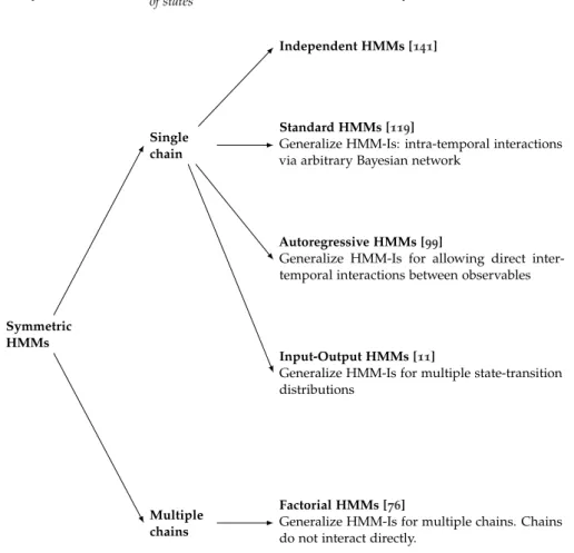
By relaxing the assumptions of the independent HMM based on the general architecture shown in Figure2.3, different families of HMMs can be derived, as
summarized in Figure2.4. The emissions of astandardHMM can be defined as:
P(X|S) =
n
∏
i=1
whereπ−(Xi)denotes the set of parents ofXiexcluding the state, and it depends
on the Bayesian network associated to the feature space. In the literature, the standard HMM is also known as HMM/BN [119].
Symmetric HMMs
Single chain
Standard HMMs [119]
Generalize HMM-Is: intra-temporal interactions via arbitrary Bayesian network
Independent HMMs [141]
Autoregressive HMMs [99]
Generalize HMM-Is for allowing direct inter-temporal interactions between observables
Input-Output HMMs [11]
Generalize HMM-Is for multiple state-transition distributions
Multiple chains
Factorial HMMs [76]
Generalize HMM-Is for multiple chains. Chains do not interact directly.
Probabilistic modularity Chain
of states Family
Figure2.4: HMM families, whereintra-temporalinteractions refer to probabilistic interac-tion among observables from the same time point, whileinter-temporal interac-tions refer to interacinterac-tions between distinct time points.
The models from Figure2.4can be distinguished based on a number of factors,
where probabilistic modularity, i.e. the sets of variables that are directly connected in the model, has a major importance. For example, the very high modularity of HMM-Is requires that the state variable summarize more history information, which can imply larger state spaces [76], as opposed to autoregressive HMMs,
2.6 l e a r n i n g w i t h l at e n t va r i a b l e s 23
2.5.3 Learning
Learning HMMs often reduces to parameter learning, because the structure of models such as the independent HMM and input-output HMM is defined before-hand. However, structure learning might be needed, e.g., for learning standard HMMs and autoregressive HMMs if one wants to decide which autoregressions should be present based on the data. Due to the presence of latent variables, learning HMMs is addressed differently than discussed so far and will be covered in more detail in Section2.6.
2.6 l e a r n i n g w i t h l at e n t va r i a b l e s
In many real-life situations the data might have variables with missing values due to several reasons, e.g., when patients drop out of treatment, do not carry out a measurement or forget to register the result of a measurement, or when a sensor breaks down. At other times, we might be interested in modeling latent (or hidden) variables, i.e., the situation when no values have been observed for a variable, which is the case of probabilistic models such as HMMs. Dealing with missing values or with situations when all values of a variable are missing is done by similar algorithms. In this section we discuss learning of models with latent variables.
Learning Bayesian networks with latent variables is more difficult than the case of complete data, as closed-form solutions are in general not available [15,21]. Iterative methods are often used, including gradient-based methods
[104] and the expectation maximization algorithm (EM, for short) [53,65,67].
More recently, research has shown that in some situations parameter learning of Bayesian networks with latent variables can be done in closed form [21], while
structure learning has been done by approximating predictive distributions, also in an iteration-free approach [143].
2.6.1 The expectation-maximization algorithm
In the situation of latent variables, the space of variables is given by a set of observablesXtogether with a set of latent variablesS. Then, the log-likelihood function of model parametersθgiven a probabilistic structureP(X:θ)and data
onXcan be written as:
logL(θ:x) =logP(x:θ) =log
∑
sP(x,s:θ) (2.28)
The presence of the summation inside the logarithm makes it difficult to optimize Equation2.28analytically, because the marginalP(x:θ)might not belong to the
exponential family even if P(x,s:θ) does [15]. The expectation maximization
resorts to the expected likelihood of the complete data. A general description of the EM procedure is provided in Algorithm1. In the context of (dynamic)
Bayesian networks, the described EM algorithm assumes the network structure is known and the goal is to perform parameter estimation, thusθrefers to model
parameters.
Algorithm1Expectation-maximization algorithm.
Input: D: a set of data points of the formX={X1, . . . ,Xn};S={S1, . . . ,S`}:
a set of latent variables.
Output: θ: model parameters for the distributionP(x,s).
1: Choose initial model parametersθold.
2: repeat
3: E step: ComputeP(s|x:θold)
4: M step: Computeθnew as follows:
θnew←arg max
θ
Q(θ,θold) (2.29)
where Q(θ,θold)def= Es h
logP(x,s:θ)|x:θold i
(2.30)
=
∑
s
P(s|x:θold)logP(x,s:θ) (2.31)
θold←θnew (2.32)
5: untilconvergence of the log-likelihood or the model parameters is achieved
6: returnθnew
The goal of Algorithm 1 is to maximize the expected log-likelihood with
regard to the latent states (Equation2.30) in an iterative way. Algorithm1starts
with initial model parameters θ0, which is often randomly generated. Then,
EM calculates the term of Equation2.30 regarding the current parameters, i.e.
P(s|x:θold), which is known as theE step. Once this is done, it is possible to
evaluate candidate model parameters for the expected log-likelihood. The goal now is to find new model parameters that optimizes this expectation, which is known as theM step. The process of generating new model parameter estimates from the current one is repeated until no improvement is possible, which means that a local maxima or a saddle point of the likelihood function has been achieved [65]. It is possible to show [15] that each cycle of E and M steps generates a new
2.6 l e a r n i n g w i t h l at e n t va r i a b l e s 25
2.6.2 The Baum-Welch algorithm
Models with latent variables such as HMMs are often learned by means of the EM algorithm, which is also known as the Baum-Welch algorithm in this context [141]. In this section, we consider the learning of HMMs with fixed structure,
for which learning reduces to parameter learning. We use independent HMMs to illustrate the necessary calculations. These involve estimating the parameters
θ, which include the emission distributions P(X(it) | S(t)), with Xi ∈ X and
dom(S) ={s1, . . . ,sk}, the transitionsP(S(t+1)|S(t))and the initial probabilities
P(S(0)).
We consider the same learning setting as that of learning DBNs (Section2.4.2),
but in order to simplify the notation, we consider that the data Dconsists of a single sequence over {0, . . . ,T}. This can be easily extended to the case of multiple i.i.d. sequences. Let us denote byθold the parameters of current HMM-I
and by θ the parameters of new HMM-I to be obtained. The Q function of
Equation2.30for HMMs becomes:
Q(θ,θold) =
∑
s(0:T)
P(s(0:T),x(0:T):θold)·logP(x(0:T),s(0:T):θ) (2.33)
For convenience, in Equation2.33the jointP(s,x:θold)was used. It holds that
P(s,x:θold) = P(x:θold)P(s| x:θold), thus one can use either the joint or the
conditional probability for this development because they are independent ofθ.
By substituting the joint of HMMs (Equation2.26) into Equation2.33, we obtain:
Q(θ,θold) =
∑
s(0:T)
P(s(0:T),x(0:T):θold)·logP(s(0))
+
∑
s(0:T)
P(s(0:T),x(0:T):θold)
T
∑
t=0 n
∑
i=1
logP(X(it)|s(t))
!
+
∑
s(0:T)
P(s(0:T),x(0:T):θold)
T−1
∑
t=0
logP(s(t+1)|s(t))
!
(2.34)
In order to maximize suchQfunction, one can maximize each term independently. The term referring to the initial distribution can be written as:
∑
s(0:T)
P(s(0:T),x(0:T):θold)·logP(s(0)) (2.35)
=
∑
s(0:T)
P(s(0:T),x(0:T):θold)·logυ(i) (2.36)
By setting the derivative with respect to υ(i) to zero, and introducing the
Lagrangeαmultiplier to ensure the constraint∑ki=1υ(i) =1 we obtain: ∂
∂υ
∑
s(0:T)
P(s(0:T),x(0:T):θold)·logυ(i)−α(
k
∑
i=1
υ(i)−1) !
It is possible to show [14] that this results in:
υ(i) = P(x
(0:T),s(0)
i :θold)
P(x(0:T):θold) (2.38)
By similar reasoning we obtain the transitions and emissions:
aij = ∑T−1
i=0 P(x(0:T),s
(t)
i ,s
(t+1)
j :θold) ∑T−1
i=0 P(x(0:T),s
(t)
i :θold)
(2.39)
bj(k) =
∑T
i=0P(x(0:T),s
(t)
j :θold)·1(k)
∑T
i=0P(x(0:T),s
(t)
j :θold)
(2.40)
where1(k) =1 ifX(t)=xk, and 0 otherwise.
In order to actually compute the above probabilities, some useful quantities are defined:
γt(i)def= P(s(it)|x(0:T):θold) (2.41)
ξt(i,j)def= P(s(it),sj(t+1)|x(0:T):θold) (2.42)
In many families of HMMs, theγandξvalues can be efficiently computed by
the forward-backward procedure based on dynamic programming [14,15]. This
fact is important for keeping the EM iterations efficient. Then, it is possible to show [141] that parameter update leads toθnew= (A,B,v)given by:
υ(i) =γ0(i) (2.43)
aij= ∑ T−1 t=0 ξt(i,j)
∑T−1 t=0 γt(i)
(2.44)
bj(k) = ∑ T
t=0γt(j)·1(k)
∑T
t=0γt(j)
(2.45)
2.6.3 Number of latent states
One important hyperparameter of HMMs is the number of latent states. It is often the case that this hyperparameter is not known in advance, hence one can resort to estimating it using data. Information-theoretic criteria, such as AIC and BIC, can be used for this task [35,138], with the advantage of low computational