REVISITING THE STATISTICAL RELATIONSHIP BETWEEN
SOLAR ACTIVITY AND ASIAN MONSOON DURING THE
HOLOCENE
Yue Zhang
A thesis submitted to the faculty of the University of North Carolina at Chapel Hill in partial fulfillment of the requirements for the degree of Master of Science in the Department of Geological Sciences (Geophysics).
Chapel Hill 2012
Approved by: Donna M. Surge John M. Bane
ii © 2012 Yue Zhang
iii ABSTRACT
YUE ZHANG: REVISITING THE STATISTICAL RELATIONSHIP BETWEEN SOLAR ACTIVITY AND ASIAN MONSOON DURING THE HOLOCENE
(Under the direction of Donna M. Surge)
iv
v
ACKNOWLEDGEMENTS
I would never have been able to finish my thesis without the guidance of my committee members. Foremost, I would like to express my sincere gratitude to my advisor Dr. Donna Surge for the continuous support, advice and encouragement throughout my research. One simply could not wish for a better or friendlier advisor. Second, I would like to thank the rest of my committee members, Dr. John Bane and Dr. Jonathan Lees, for their insightful comments and encouragement. I sincerely appreciate their patience to answer my questions when I attended their Geophysical Fluid Dynamics and Data Analysis in the Earth Sciences classes.
Moreover, I would like to show my sincere thanks to Deborah Harris and Elizabeth Mullane for their help to make the department run smoothly and for their assistance in many different ways. I am also grateful to Dr. Allen Glazner, Dr. Leslie Lerea and Anne Schwarz for their strong support in my hard time.
Besides, I would like to thank my colleague Ting Wang for her help and encouragement in many aspects. It is a great pleasure to share an office with her. Also, thank all fellow students in UNC geology. It is an honor to enjoy two-year indelible time with you all in this great university.
vi
In addition, I would like to thank Ambrose Chiang, David Stickel, Yan Wang and Jun Xiong for their help in my living. Thank all my friends and people who gave me help. For them, I don’t feel lonely.
vii
TABLE OF CONTENTS
LIST OF TABLES --- ix
LIST OF FIGURES --- x
LIST OF ABBREVIATIONS --- xii
LIST OF SYMBOLS --- xiii
Chapter I Revisiting the statistical relationship between solar activity and Asian monsoon during the Holocene --- 1
Abstract --- 1
Introduction --- 2
Data and methods --- 8
Data --- 8
Ensemble empirical mode decomposition (EEMD) --- 9
Wavelet coherence (WTC) --- 12
Significance test --- 14
IMF --- 16
Coherence and phase relationship --- 17
∆14C and δ18Ospeleothem values --- 18
Total solar irradiance and δ18Ospeleothem values --- 19
viii
ix
LIST OF TABLES
Table
1. Periods for IMFs of atmospheric ∆14C and DA δ18Ospeleothem record --- 22
x
LIST OF FIGURES
Figure
1. Atmospheric ∆14C over the last 8,800 years --- 24
2. Total solar irradiance over the last 8,800 years --- 25
3. Stalagmite DA δ18O from Dongge Cave, China, over the last 8,800 years --- 26
4. IMFs and the trend of atmospheric ∆14C --- 27
5. IMFs and the trend of total solar irradiance --- 28
6. IMFs and the trend of DA δ18Ospeleothem --- 29
7. Significance test of IMFs of atmospheric ∆14C --- 30
8. Significance test of IMFs of total solar irradiance --- 31
9. Significance test of IMFs of DA δ18Ospeleothem --- 32
10. Instantaneous frequency of atmospheric ∆14C IMF2-8 --- 33
11. Instantaneous frequency of total solar irradiance IMF2-8 --- 34
12. Instantaneous frequency of DA δ18Ospeleothem IMF2-8 --- 35
13. Comparison for frequency distribution of corresponding IMF2-8 --- 37
14. WTC for IMF2 of atmospheric ∆14C and DA δ18Ospeleothem --- 38
15. WTC for IMF3 of atmospheric ∆14C and DA δ18Ospeleothem --- 39
16. WTC for IMF4 of atmospheric ∆14C and DA δ18Ospeleothem --- 40
xi
18. WTC for IMF6 of atmospheric ∆14C and DA δ18Ospeleothem --- 42
19. WTC for IMF7 of atmospheric ∆14C and DA δ18Ospeleothem --- 43
20. WTC for IMF2 of total solar irradiance and DA δ18Ospeleothem --- 44
21. WTC for IMF3 of total solar irradiance and DA δ18Ospeleothem --- 45
22. WTC for IMF4 of total solar irradiance and DA δ18Ospeleothem --- 46
23. WTC for IMF5 of total solar irradiance and DA δ18Ospeleothem --- 47
24. WTC for IMF6 of total solar irradiance and DA δ18Ospeleothem --- 48
25. WTC for IMF7 of total solar irradiance and DA δ18Ospeleothem --- 49
xii
LIST OF ABBREVIATIONS
AD Anno Domini
AR1 first-order autoregressive BP Before Present
COI Cone of Influence
CWT Continuous Wavelet Transform EMD Empirical Mode Decomposition
EEMD Ensemble Empirical Mode Decomposition et al. et alia
etc et cetera
GRIP Greenland Ice Core Project i.e. id est
IMF Intrinsic Mode Function kyr kiloyear
xiii
LIST OF SYMBOLS
10
Be beryllium isotope 10 14
C radiocarbon isotope 14 13
C carbon isotope 13 12
C carbon isotope 12 ∆14C ratio of 14C to 12C CO2 carbon dioxide
DA a stalagmite sample from Dongge Cave 14
N nitrogen isotope 14 18
O oxygen isotope 18 16
O oxygen isotope 16
δ18O delta notation of the 18O:16O ratio of a sample relative to a standard 230
Th thorium isotope 230
Revisiting the statistical relationship between solar activity
and Asian monsoon during the Holocene
1Abstract
The relationship between the sun and terrestrial climate in the past has been controversial. Given the difficulty in understanding the underlying mechanism(s) of solar influence on the climate system, the empirical relationship between the sun and climate variables relies on statistical analyses. The tight link between proxies for solar irradiance and the Asian monsoon has gained wide consensus; however, this unresolved scientific issue is still under debate. Here, the nonlinear and nonstationary relationship between solar activity and Asian monsoon strength during the last 8,800 years is investigated with Ensemble Empirical Mode Decomposition (EEMD) and Wavelet Coherence (WTC). The results show the coherence between solar activity and Asian monsoon strength is low in time-frequency-oscillatory mode representation. There is no causal relationship between solar activity and Asian monsoon strength during the Holocene that can be identified. This research provides a new insight into the sun-Asian monsoon interaction.
1
2
Introduction
The Earth’s climate is controlled by external forcings and internal processes. As the heat engine of the Earth’s climate system, the sun is the most dominant external forcing and is considered to affect climate variability in the past, present and future (Beer et al., 2000; Crowley, 2000; Bond et al., 2001; Haigh, 2001; Shindell et al., 2001; Rind, 2002; Gimeno et al., 2003; Braun et al., 2005). Accurate reconstruction of past climate change is critical to projecting future climate changes (Gray et al., 2010). Thus, characterizing the contribution of solar activity to climate variability over disparate timescales has been a focus of study for the last several decades. However, long-term observation of solar activity is sparse. Telescopic observations of sunspot numbers extend from the present back to AD 1610, while satellite monitoring of total solar irradiance only began in 1978 (Solanki et al., 2004). Reconstructing the variation of solar activity over geological timescales (in particular, during the Holocene) relies on proxy records of solar activity, such as various cosmogenic radionuclides (e.g., 10Be and 14C). Similarly, climate variability that occurred before the era of instrumental observation is typically reconstructed using proxy records such as ice cores, tree rings, marine sediments, speleothems, archaeological and fossil shells, etc. Hence, dynamical links between solar activity and past climate variability are often proposed based on the statistical relationships between proxies for solar activity and those for past climate change (Legras et al., 2010; Yiou et al., 2010).
3
4
5
influence of the carbon cycle on 14C variation can overcome the effect of solar activity (Bradley, 1999). Moreover, the terrestrial biosphere plays a key role in the global carbon cycle (Hahn and Buchmann, 2004; Naegler and Levin, 2009). Radiocarbon in fossil fuelis low owing to radioactive decay. Burning of fossil fuel makes 13C and 12C become more enriched in the atmosphere. Accordingly, human use of fossil fuel can also greatly reduce ∆14C over the globe (Suess, 1955). Hence, atmospheric ∆14C is dominated by both 14C production rate, and climate-related, and human-induced processes (Kitagawa and van der Plicht, 1998). It is not a pure proxy for solar activity in the past.
6
consecutive fractionation processes at water phase transitions (i.e., condensation and evaporation) in the hydrological cycle (Araguas-Araguas et al., 1998; Jouzel et al., 2000; Johnson and Ingram, 2004). Therefore, δ18O values recorded in speleothems represent several factors rather than simply Asian monsoon strength (Lachniet, 2009). In summary, both ∆14C and δ18Ospeleothem values are composite signals, as opposed to pure indicators of climate variables. Accordingly, the direct comparison between two complicated signals may not clearly reveal the underlying mechanisms of solar influence on the Asian monsoon.
7
insolation variability caused by long-term changes in Earth’s orbital parameters leads the marine δ18O record (indicating ice volume variations) by 90 degrees on orbital time scales, which is 10,000 years for obliquity band and 6,000 years for precession band (Ruddiman, 2007). As a weather system, the Asian monsoon’s response to variation of solar irradiance is much slower than that of temperature and much faster than that of ice sheets because of a series of complex physical processes and feedbacks. Hence, the phase angle between solar activity and Asian monsoon is expected to be between 45 and 90 degrees. Moreover, ∆14C should not be in phase with δ18Ospeleothem values, but rather should lead it. A strong correspondence may be unreasonable to expect.
Haam and Huybers (2010) measured the linear and in-phase covariance between atmospheric ∆14C and stalagmite DA δ18O from Dongge Cave with a novel methodology for
maximum covariance test of time-uncertain series. They suggested that the correlation coefficient of 0.3 between solar activity and Asian monsoon strength reported by Wang et al. (2005) is insignificant at the 95% confidence level. This implies that there might be no causal relationship between solar activity and Asian monsoon strength during the Holocene. However, a nonlinear and nonstationary link between solar activity and Asian monsoon strength cannot be ruled out based solely on their analysis.
8
solar influence on the Asian monsoon. The proxy records for both solar irradiance and the Asian monsoon (∆14C and δ18Ospeleothem) are composite signals superimposed by various underlying processes in the climate system. As proxy records, it is assumed that ∆14C and δ18Ospeleothem time series contain information of past solar and Asian monsoon activity. If the Asian monsoon is paced unidirectionally by the sun during the Holocene, the sun should leave a signature in both the ∆14C and δ18Ospeleothem records. ∆14C and δ18Ospeleothem time series
should contain similar underlying processes with similar periods and appropriate phase relations. Following this rationale, time series for atmospheric ∆14C, total solar irradiance
(reconstructed from 10Be accumulated in ice cores), and δ18Ospeleothem are decomposed into inherent components using Ensemble Empirical Mode Decomposition (EEMD), a newly applied procedure in paleoclimatology. Wavelet Coherence (WTC) is then employed to quantify the coherence and phase relationship between the corresponding processes from the EEMD results.
Data and methods Data
Previously documented records of atmospheric ∆14C, total solar irradiance, and δ18Ospeleothem are used in this study (Figures 1-3). The atmospheric ∆14C time series was
9
which is also dominated by solar activity. Total solar irradiance was computed based upon its functional relation with the open solar magnetic field (Steinhilber et al., 2009). A stalagmite DA was retrieved from Dongge Cave (25°17N, 108°5E, elevation 680m) in south China (Wang et al., 2005). The corresponding δ18O record is dominated by isotopic variations in
local meteoric water, which is further related to variations in precipitation amount characterizing Asian monsoon strength. The chronology of the Dongge Cave stalagmite was constructed using 230Th dating, and the typical age uncertainty is about 50 years. The time span of all records is from 8,800 year BP to 0 year BP. All the data linearly interpolated with a 10-year sampling interval.
Ensemble empirical mode decomposition (EEMD)
10
are connected respectively by two cubic spline curves to generate the upper and lower envelopes, where is the mean of the two envelopes and is the first component that equals the difference between and .
However, the new extrema may be generated as a result of changing the local zero from a rectangular coordinate system to a curvilinear one. Hence, needs to be sifted repeatedly to eliminate the riding waves (background signals) and make the time series more symmetric.
After k times of sifting,
The first IMF is obtained
The number of iterations, k, is determined by stoppage criteria (Huang, 2005). A typical stoppage criterion is a Cauchy type of convergence test that requires the normalized squared difference between two successive sifting processes:
∑ | | ∑
11
Because still contains oscillatory modes with lower frequencies, the sifting process can be employed again after considering as a new time series.
This is repeated until the sifting process is stopped when no IMF can be extracted from the residue .
Therefore, the original data can be represented with n IMFs and a residue .
The final residue can be considered to be a trend. Because the decomposition directly works in the temporal domain but not in the frequency domain and only relies on the local characteristics of the data, EMD can solve the nonlinearity and nonstationarity of the data. However, the EMD-produced results may have a mode-mixing problem, which is caused by signal intermittency (Huang and Wu, 2008).
12
with EMD first. Then, this procedure is repeated with distinct white noise time series. The final result in EEMD is defined as the ensemble mean of all corresponding EMD-produced IMFs. Though each time’s result is very noisy, the noise can be canceled out with averaging. Nevertheless, the EEMD results do not strictly satisfy the two conditions for IMF. Hence, one more sifting is done to eliminate the riding wave (Huang and Wu, 2008).
Wavelet coherence (WTC)
Wavelet analysis uses a zero-mean wavelet to fit a time series in both time and frequency domains (Grinsted et al., 2004). As a locally periodic wavetrain, the Morlet, a Gaussian-windowed complex sinusoid, is expressed as:
! "⁄ $%&'($()
where and * are dimensionless time and frequency, respectively. Continuous Wavelet Transform (CWT) is defined as:
+,- ./- 0
1
0
234 3/- 5
This can be seen as a convolution of a time series with a scaled and normalized wavelet, where |+,-| and the complex argument of +,- represent wavelet power and local phase, respectively. Wavelet Coherence (WTC) measures the coherence and phase relationships between two time series and is defined as:
6-
+,9-:7
13 where , a smoothing operator, defined as:
+ <=>?@A%B@8+-:C
where <=>?@ and %B@ are the smoothing in Wavelet scale and in time. For the Morlet, the smoothing operator is defined as:
D%B@+|< DE+- F )
<)GH
<
D%B@+|< DA+- F I0.6sCN
where and are normalization constants, and ∏ is a rectangle function (Torrence and Webster, 1998). The value 0.6 is a scale decorrelation length, which is decided empirically for the Morlet (Torrence and Compo, 1998).
14
Significance test
Proxy records are generally contaminated by noise. A significance test of the IMFs is necessary to estimate whether an IMF represents the true signal or only consists of noise. Wu and Huang (2004) developed a test of statistical significance based on the characteristics of white noise and the orthogonality of the IMFs. For normalized white noise, O, the energy density of the nth IMF PQ can be expressed as:
R T UP1 QV 1
The total energy is defined as:
O 1
|W| 1
T R
where X √1, O and W are respectively represented as:
O 6$ Z W$%[1 1
\ PQ
and
W O$%[1 1
Consequently, it is suggested that the energy density of an IMF and its average period satisfy a hyperbolic relationship:
15
where R___ equals the mean of R if n a ∞. If an IMF’s energy density is located above the upper spread lines of the selected confidence levels, the null hypothesis that this IMF is not distinguishable from the corresponding IMF of a white noise can be rejected. In other words, the decomposition result is statistically significant.
Here, each of the three records was decomposed into eight oscillatory components and a trend with EEMD (Figures 4-6). Then, another sifting was done on each IMF except the trend to confirm that the EEMD-produced results follow the conditions defining an IMF. Eventually, the statistical significance of each IMF (except IMF8 which is also a trend) was tested at 95% and 99% confidence levels (Figures 7-9). Empirically, the first IMF results from random noise; therefore, it is not considered in the discussion. However, it is still employed to compute the mean energy of the other IMFs.
For atmospheric ∆14C, IMF4 through IMF7 are above the 95% and 99% confidence
level lines, and are considered statistically significant. IMF2 and IMF3 located on the 95% confidence level line are still physically meaningful. For total solar irradiance, IMF2 through IMF7 are above 95% and 99% confidence level lines and are all statistically significant. For DA δ18Ospeleothem, IMF3 through IMF7 are above 95% and 99% confidence level lines and are
16
IMFs for total solar irradiance generally are more statistically significant than IMFs for atmospheric ∆14C. However, the estimation of which record best represents solar activity
is beyond the scientific scope of this study. Therefore, the comparison between them is not discussed here. Because many similarities of the corresponding IMFs from both data can be identified with visual inspection, it is considered that both of them can represent solar activity during the Holocene.
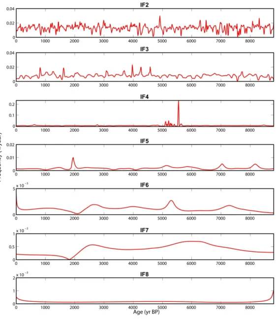
IMF
To investigate the relationship between corresponding underlying processes for solar activity and Asian monsoon strength, the period of each IMF was quantified. Prior to obtaining the period of an IMF, the instantaneous frequency of each IMF was calculated with a Hilbert transform-produced analytic function (Huang and Wu, 2008) (Figures 10-12). The Hilbert transform of a function of LP class (pth powers of must be integrable) is defined as:
b 1! c d e fee
g
g
where P is the Cauchy principal value of the singular integral. Considering the Hilbert transform as the imaginary part, the analytic signal can be expressed as:
h Xb i$%j
i b ⁄
k tanb
17
where X √1, i and k are instantaneous amplitude and phase. Instantaneous frequency then can be expressed as:
* fkf
Subsequently, a probability density function for each instantaneous frequency was estimated with a normal kernel function. The instantaneous frequency of each IMF (except IMF1) is approximately normally distributed. The frequency distributions of corresponding IMFs have similar shapes (Figure 13). For a given IMF, the frequency with the highest density value was selected as its mean frequency. The mean period of each IMF was then obtained according to the mathematic relation between period and frequency (Tables 1 and 2). The period of IMF8 is so long that it is considered a trend within the 8,800-year period under investigation. The periods of the corresponding IMFs from the three proxy records (i.e., ∆14C, total solar irradiance, and DA δ18Ospeleothem) are very similar. Given this, we hypothesize that the corresponding IMFs from the three records represent similar underlying processes within the data. Thus, WTC can be applied to each pair of the corresponding IMFs for coherence estimations. As a whole, the period of a given IMF is roughly half of that of the next IMF, which means EMD is a dyadic filter (Wu and Huang, 2004).
Coherence and phase relationship
The following data analysis is separated into two groups: (1) atmospheric ∆14C and
DA δ18Ospeleothem; and (2) total solar irradiance (reconstructed from the ice core 10Be record)
and DA δ18Ospeleothem. In the WTC plots, the high coherence between two signals is
18
against red noise. The local phase relationship is expressed by the arrows. Arrows pointing right represent in-phase, while arrows pointing left are anti-phase. If the first signal leads the second one by 90 degrees, arrows point straight up. In contrast, a 90-degree lag corresponds
to the arrows pointing straight down. For a lead-lag relationship, only coherence areas with proper phase angle (45-90 degrees; i.e., the range between the diurnal/seasonal cycle and ice volume, respectively) are identified. Due to the edge artifacts, high coherence areas outside the COI or penetrating the COI are not meaningful. Hence, only high coherence areas with correct phase angles are presented in following sections.
∆ ∆ ∆
∆14C and δδδδ18Ospeleothem values
For IMF2, high coherence appears at 22-48 yr around 900-1000 yr BP, at 24-60 yr around 2000-2350 yr BP, at 24-40 yr around 3500-3600 yr BP, at 20-32 yr around 3800 yr BP, at 256-374 yr around 5250-6100 yr BP, at 20-40 yr around 5400-5500 yr BP, at 40-64 yr around 6500 yr BP, and at 50-128 yr around 7950-8500 yr BP (Figure 14). For IMF3, high coherence occurs at 32-60 yr around 6400 yr BP, at 256-384 yr around 7200-8200 yr BP, at 48-100 yr around 8000 yr BP, and at 40-56 yr around 8400 yr BP (Figure 15). For IMF4, high coherence is shown at 200-320 yr around 7200-8000 yr BP (Figure 16). For IMF5, high coherence is present at 64-96 yr around 750 yr BP and at 224-384 yr around 5100-5600 yr BP (Figure 17). For IMF6, there is high coherence at 100-192 yr around 4300-4750 yr BP and at 64-90 yr around 8000-8200 yr BP (Figure 18). IMF7 has no coherence (Figure 19). In sum, in time-frequency-IMF representation, the coherence between atmospheric ∆14C and
19
Total solar irradiance and δδδδ18Ospeleothem values
For IMF2, high coherence is indicated at 24-56 yr around 7500-7600 yr BP (Figure 20). For IMF3, high coherence appears at 48-64 yr around 4750-4900 yr BP and at 48-80 yr around 5800-6000 yr BP (Figure 21). For IMF4, high coherence appears at 128-200 yr around 1250-1500 yr BP (Figure 22). For IMF5, high coherence occurs at 300-448 yr around 3500-4000 yr BP (Figure 23). For IMF6, no significant coherence is detected (Figure 24). For IMF7, there is high coherence at 340-426 yr around 5500-5900 yr BP and at 96-128 yr around 7200-7500 yr BP (Figure 25). Thus, in time-frequency-IMF representation, the coherence between total solar irradiance and DA δ18Οspeleothem is low.
Discussion
Our results demonstrate a weak link between solar activity and the Asian monsoon strength over the last 8,800 years, which is exemplified by low coherence in time-frequency-IMF representation. Previously reported causal links also rely on the frequency spectrum (Fleitmann et al., 2003; Wang et al., 2005; Cai et al., 2010). Wang et al. (2005) reported correlation at specific frequencies between detrended atmospheric ∆14C and DA δ18Ospeleothem
values with bivariate spectral analysis (see supporting online material for Wang et al. (2005)). The phase spectrum between detrended atmospheric ∆14C and DA δ18Ospeleothem values was
not discussed. As a complement, the cross-coherence and phase spectrum between atmospheric ∆14C and DA δ18Ospeleothem raw data are also measured in the present study. For
20
Stattegger, 1997; Wang et al., 2005). The correspondence between atmospheric ∆14C and DA δ18Ospeleothem at each frequency is expressed with the squared coherency, which is estimated
with Lomb-Scargle Fourier transform for unevenly spaced time series, associated with a Welch-Overlapped-Segment-Averaging procedure. The value of the squared coherency ranges between 0 and 1, in which 0 means no correlation and 1 presents highest correlation at the corresponding frequencies. Overall, the coherence between atmospheric ∆14C and DA δ18Ospeleothem is not high. High coherence with 95% false alarm level only occurs at 57 and 20
yr in which the squared coherency equals 0.45 and 0.54 respectively (Figure 26). For the phase spectrum (figure is not shown), ∆14C leads DA δ18Ospeleothem values by -109 degrees at
57 yr and 28 degrees at 20 yr. In sum, the spectral coherency between atmospheric ∆14C and
DA δ18Ospeleothem is low, and the phase angles are not meaningful.
Conclusions
Insignificant covariance between atmospheric ∆14C and DA δ18Ospeleothem record at the
21
strength over the last 8,800 years is insignificant. Our study supports that a causal relationship does not exist between solar activity and Asian monsoon strength during the Holocene.
Acknowledgements
22
Table 1. Periods for IMFs of atmospheric ∆14C and DA δ18Ospeleothem record
∆14C δ18O
Components Period (year) Components Period (year)
IMF2 73 ± 344 IMF2 72 ± 430
IMF3 124 ± 553 IMF3 141 ± 566
IMF4 258 ± 674 IMF4 238 ± 943
IMF5 658 ± 1812 IMF5 575 ± 3017
IMF6 864 ± 2591 IMF6 1206 ± 3810
IMF7 2380 ± 4454 IMF7 2508 ± 14388
23
Table 2. Periods for IMFs of total solar irradiance and DA δ18Ospeleothem record
Total solar irradiance δ18O
Components Period (year) Components Period (year)
IMF2 79 ± 284 IMF2 72 ± 430
IMF3 144 ± 522 IMF3 141 ± 566
IMF4 286 ± 1411 IMF4 238 ± 943
IMF5 818 ± 1757 IMF5 575 ± 3017
IMF6 1448 ± 6849 IMF6 1206 ± 3810
IMF7 2236 ± 11364 IMF7 2508 ± 14388
24
25
26
Figure 3. Stalagmite DA δ18O from Dongge Cave, China, over the last 8,800 years (Wang et
27
Figure 4. IMFs and the trend of atmospheric ∆14C. In EEMD, the ratio of white noise’s stand
30
Figure 7. Significance test of IMFs of atmospheric ∆14C. Since IMF1 is a random noise, it is
31
32
Figure 9. Significance test of IMFs of DA δ18Ospeleothem. IMF3 through IMF7 are above 95%
33
34
35
37
Figure 13. Comparison for frequency distribution of corresponding IMF2-8 (red: ∆14C,
38
Figure 14. WTC for IMF2 of atmospheric ∆14C and DA δ18Ospeleothem. The area with the thick
contour indicates high coherence. The contour means the 0.05 significance level against red noise. The local phase relationship is expressed by the arrows. Arrows pointing right are in-phase, while arrows pointing left are anti-phase. The first signal leading the second one by
90 degrees results in arrows pointing straight up, while a 90-degree lag corresponds to the
39
Figure 15. WTC for IMF3 of atmospheric ∆14C and DA δ18Ospeleothem. High coherence occurs
40
Figure 16. WTC for IMF4 of atmospheric ∆14C and DA δ18Ospeleothem. High coherence is
41
Figure 17. WTC for IMF5 of atmospheric ∆14C and DA δ18Ospeleothem. High coherence is
42
Figure 18. WTC for IMF6 of atmospheric ∆14C and DA δ18Ospeleothem. There is high
43
44
Figure 20. WTC for IMF2 of total solar irradiance and DA δ18Ospeleothem. High coherence is
45
Figure 21. WTC for IMF3 of total solar irradiance and DA δ18Ospeleothem. High coherence
46
Figure 22. WTC for IMF4 of total solar irradiance and DA δ18Ospeleothem. High coherence
47
Figure 23. WTC for IMF5 of total solar irradiance and DA δ18Ospeleothem. High coherence
48
Figure 24. WTC for IMF6 of total solar irradiance and DA δ18Ospeleothem. No significant
49
Figure 25. WTC for IMF7 of total solar irradiance and DA δ18Ospeleothem. There is high
50
Figure 26. Coherency between atmospheric ∆14C and DA δ18Ospeleothem. The oversampling
factor is 3, factor for highest frequency is 1 and false alarm level is 95% (dashed line). A Welch I window with 50% overlapping is employed to divide the signal into 8 segments in which linear trend of each segment is removed. At 57 yr and 20 yr, ∆14C leads δ18O values
51
References
Agnihotri, R., Dutta, K., Bhushan, R., and Somayajulu, B. L. K.: Evidence for solar forcing of the southwest monsoon during the last millennium, Earth Planet. Sci. Lett., 198, 521-527, 2002.
Araguás-Araguás, L., Froehlich, K., and Rozanski, K.: Stable isotope composition of precipitation over southeast Asia, J. Geophys. Res., 103(D22), 28, 721-28, 742, 1998.
Beer, J., Mende, W., and Stellmacher, R.: The role of the Sun in climate forcing, Quaternary Sci. Rev., 19, 403-415, 2000.
Bond, G., Kromer, B., Beer, J., Muscheler, R., Evans, M. N., Showers, W., Hoffmann, S., Lotti-Bond, R., Hajdas, I., and Bonani, G.: Persistent Solar Influence on North Atlantic Climate During the Holocene, Science, 294, 2130-2136, 2001.
Bradley, R. S.: Paleoclimatology: Reconstructing Climates of the Quaternary. Academic Press, San Diego, 1999.
Braun, H., Christl, M., Rahmstorf, S., Ganopolski, A., Mangini, A., Kubatzki, C., Roth, K., and Kromer, B.: Possible solar origin of the 1470-year glacial climate cycle demonstrated in a coupled model, Nature, 438, 208-211, 2005.
Burke, A., and Robinson, L. F.: The Southern Ocean’s Role in Carbon Exchange During the Last Deglaciation, Science, 335(6068), 557-561, 2012.
Cai, Y., Tan, L., Cheng, H., An, Z., Edwards, R. L., Kelly, M. J., Kong, X., and Wang, X.: The variation of summer monsoon precipitation in central China since the last deglaciation, Earth Planet. Sci. Lett., 291, 21-31, 2010.
Clemens, S. C.: Millennial-band climate spectrum resolved and linked to centennial-scale solar cycles, Quaternary Sci. Rev., 24, 521-531, 2005.
Crowley, T. J.: Causes of climate change over the past 1000 years, Science, 289, 270-277, 2000.
Dykoski, C. A., Edwards, R. L., Cheng, H., Yuan, D., Cai, Y., Zhang, M., Lin, Y., Qing, J., An, Z., and Revenaugh, J.: A high-resolution, absolute-dated Holocene and deglacial Asian monsoon record from Dongge Cave, China, Earth Planet. Sci. Lett., 233, 71-86, 2005.
Fleitmann, D., Burns, S. J., Mudelsee, M., Neff, U., Kramers, J., Mangini, A., Matter, A.: Holocene forcing of the Indian monsoon recorded in a stalagmite from Southern Oman, Science, 300, 1737-1739, 2003.
Gimeno, L., de la Torre, L., Nieto, R., García, R., Hernández, E., and Ribera, P.: Changes in the relationship NAO–Northern hemisphere temperature due to solar activity, Earth Planet. Sci. Lett., 206, 15-20, 2003.
52
Grinsted, A., Moore, J. C., and Jevrejeva, S.: Application of the cross wavelet transform and wavelet coherence to geophysical time series, Nonlin. Processes Geophys., 11, 561-566, 2004.
Gupta, A. K., Das, M., and Anderson, D. M.: Solar influence on the Indian summer monsoon during the Holocene, Geophys. Res. Lett., 32, L17703, 2005.
Haam, E. and Huybers, P.: A test for the presence of covariance between time uncertain series of data with application to the Dongge Cave speleothem and atmospheric radiocarbon records, Paleoceanography, 25, PA2209, 2010.
Hahn, V. and Buchmann, N.: A new model for soil organic carbon turnover using bomb carbon, Global Biogeochem. Cy., 18, GB1019, 2004.
Haigh, J.: Climate variability and the influence of the sun, Science, 294, 2109-2111, 2001. Higginson, M. J., Altabet, M. A., Wincze, L., Herbert, T. D., and Murray, D. W.: A solar (irradiance) trigger for millennial-scale abrupt changes in the southwest monsoon?, Paleoceanography, 19, PA3015, 2004.
Hong, Y. T., Wang, Z. G., Jiang, H. B., Lin, Q. H., Hong, B., Zhu, Y. X., Wang, Y., Xu, L. S., Leng, X. T., and Li, H. D.: A 6000-year record of changes in drought and precipitation in northeastern China based on a δ13C time series from peat cellulose, Earth Planet. Sci. Lett.,
185, 111-119, 2001.
Huang, N. E. and Shen S. S. P. (Eds.): Hilbert-Huang Transform and Its Applications. World Scientific., Singapore, 2005.
Huang, N. E. and Wu, Z.: A review on Hilbert-Huang transform: Method and its applications to geophysical studies, Rev. Geophys., 46, RG2006, 2008.
Hughen, K. A., Lehman, S. J., Southon, J., Overpeck, J. T., Marchal, O., Herring, C., and Turnbull, J.: 14C Activity and Global Carbon Cycle Changes over the Past 50,000 Years, Science, 303, 202-207, 2004.
IPCC: Climate Change 2007: The Physical Science Basis, Contribution of Working Group I to the Fourth Assessment Report of the Intergovernmental Panel on Climate Change, edited by: Solomon, S., Qin, D., Manning, M., Chen, Z., Marquis, M., Averyt, K. B., Tignor, M., and Miller, H. L., Cambridge University Press, Cambridge, United Kingdom and New York, NY, USA, 996 pp., 2007.
Johnson, K. R. and Ingram, B. L.: Spatial and temporal variability in the stable isotope systematics of modern precipitation in China: implications for paleoclimate reconstructions, Earth Planet. Sci. Lett., 220, 365-377, 2004.
Jouzel, J., Hoffmann, G., Koster, R. D., and Masson, V.: Water isotopes in precipitation: Data/model comparison for present-day and past climates, Quaternary Sci. Rev., 19, 363-379, 2000.
53
Legras, B., Mestre, O., Bard, E., and Yiou, P.: A critical look at solar-climate relationships from long temperature series, Clim. Past, 6, 745-758, 2010.
Marchitto, T. M., Lehman, S. J., Ortiz, J. D., Fluckiger, J., and Van Geen, A.: Marine Radiocarbon Evidence for the Mechanism of Deglacial Atmospheric CO2 Rise, Science, 316, 1456-1459, 2007.
Mazaud, A., Laj, C., Bard, E., Arnold, M., and Tric, E.: Geomagnetic field control of 14C production over the last 80 ky: Implications for the radiocarbon time-scale, Geophys. Res. Lett., 18(10), 1885-1888, 1991.
Muscheler, R., Beer, J., Wagner, G., and Finkel, R. C.: Changes in deep-water formation during the Younger Dryas event inferred from 10Be and 14C records, Nature, 408(6812), 567-570, 2000.
Muscheler, R., Joos, J., Beer, J., Muller, S., Vonmoos, M., and Snowball, I.: Solar activity during the last 1000 yr inferred from radionuclide records, Quaternary Sci. Rev., 26, 82-97, 2007.
Naegler, T. and Levin, I.: Biosphere-atmosphere gross carbon exchange flux and the δ13CO2 and ∆14CO2 disequilibria constrained by the biospheric excess radiocarbon inventory, J. Geophys. Res., 114, D17303, 2009.
Neff, U., Burns, S. J., Mangini, A., Mudelsee, M., Fleitmann, D., and Matter, A.: Strong coherence between solar variability and the monsoon in Oman between 9 and 6 kyr ago, Nature, 411, 290-293, 2001.
Rind, D.: The Sun's role in climate variations, Science, 296, 673-678, 2002.
Rose, K. A., Sikes, E. L., Guilderson, T. P., Shane, P., Hill, T. M., Zahn, R., and Spero, H. J.: Upper-ocean-to-atmosphere radiocarbon offsets imply fast deglacial carbon dioxide release, Nature, 466, 1093-1097, 2010.
Ruddiman, W. F.: Earth’s Climate: Past and Future. W. H. Freeman & Company, New York, 2007.
Schulz, M. and Stattegger, K.: SPECTRUM: Spectral analysis of unevenly spaced paleoclimatic time series, Comput. Geosci., 23, 929-945, 1997.
Shindell, D. T., Schmidt, G. A., Mann, M. E., Rind, D., and Waple, A.: Solar forcing of regional climate change during the Maunder Minimum, Science, 294, 2149-2152, 2001. Skinner, L. C., Fallon, S., Waelbroeck, C., Barker, S., and Michel, E.: Ventilation of the deep southern ocean and deglacial CO2 rise, Science, 328, 1147-1151, 2010.
Solanki, S. K., Usoskin, I. G., Kromer, B., Schüssler, M., and Beer, J.: Unusual activity of the Sun during recent decades compared to the previous 11,000 years, Nature, 431, 1084-1087, 2004.
Staubwasser, M., Sirocko, F., Grootes, P. M., and Segl, M.: Climate change at the 4.2 ka BP termination of the Indus valley civilization and Holocene south Asian monsoon variability, Geophys. Res. Lett., 30(8), 1425, 2003.
54
Steinhilber, F., Beer, J., and Fröhlich, C.: Total solar irradiance during the Holocene, Geophys. Res. Lett., 36, L19704, 2009.
Stocker, T. F. and Wright, D. G.: Rapid changes in ocean circulation and atmospheric radiocarbon, Paleoceanography, 11(6), 773-795, 1996.
Stuiver, M., Reimer, P. J., Bard, E., Beck, J. W., Burr, G. S., Hughen, K. A., Kromer, B., McCormac, G., van der Plicht, J., and Spurk, M.: INTCAL98 radiocarbon age calibration, 24,000-0 cal BP, Radiocarbon, 40, 1041-1083, 1998.
Suess, H. E.: Radiocarbon concentrations in modern wood, Science, 122, 415-417, 1955. Torrence, C. and Compo, G. P.: A practical guide to wavelet analysis, Bull. Am. Meteorol. Soc., 79, 61-78, 1998.
Torrence, C. and Webster, P.: Interdecadal Changes in the ESNO-Monsoon System, J. Clim., 12, 2679-2690, 1999.
Wang, L., Sarnthein, M., Erlenkeuser, H., Grimalt, J., Grootes, P., Heilig, S., Ivanova, E., Kienast, M., Pelejero, C., and Pflaumann, U.: East Asian monsoon climate during the late Pleistocene: high-resolution sediment records from the South China Sea, Mar. Geol., 156, 245-284, 1999.
Wang, Y., Cheng, H., Edwards, R. L., He, Y., Kong, X., An, Z., Wu, J., Kelly, M. J., Dykoski, C. A., and Li, X.: The Holocene Asian monsoon: Links to solar changes and North Atlantic climate, Science, 308, 854-857, 2005.
Wu, Z. and Huang, N. E.: A study of the characteristics of white noise using the Empirical Mode Decomposition method,Proc. Roy. Soc. London Ser. A, 460, 1597-1611, 2004.
Wu, Z. and Huang N. E.: Ensemble Empirical Mode Decomposition: a noise-assisted data analysis method, COLA Technical Report 193, 2005.
Xiao, S. B., Li, A. C., Liu, J. P., Chen, M. H., Xie, Q., Jiang, F. Q., Li, T. G., Xiang, R., and Chen, Z.: Coherence between solar activity and the East Asian winter monsoon in the past 8000 years from Yangtze River-derived mud in the East China Sea, Palaeogeogr., Palaeoclimatol., 237, 293-304, 2006.
Yiou, P., Bard, E., Dandin, P., Legras, B., Naveau, P., Rust, H. W., Terray, L., and Vrac, M.: Statistical issues about solar-climate relations, Clim. Past, 6, 565-573, 2010.
Yuan, D., Cheng, H., Edwards, R. L., Dykoski, C. A., Kelly, M. J., Zhang, M., Qing, J., Lin, Y., Wang, Y., Wu, J., Dorale, J. A., An, Z., and Cai, Y.: Timing, duration and transitions of the last interglacial Asian monsoon, Science, 304, 575-578, 2004.