TRAVERSING THE ELASTIC LANDSCAPE WITH THE POLYMER BRUSH ARCHITECTURE: LESSONS IN THE PURSUIT OF NATURE
Andrew Nicolas Keith
A dissertation submitted to the faculty at the University of North Carolina at Chapel Hill in partial fulfillment of the requirements for the degree of Doctor of Philosophy in the
Department of Chemistry.
Chapel Hill 2020
© 2020
iii
ABSTRACT
Andrew Nicolas Keith: Traversing the Elastic Landscape with the Polymer Brush Architecture: Lessons in the Pursuit of Nature
(Under the direction of Sergei Sheiko)
This dissertation draws inspiration from the unique mechanical properties of living tissue to develop a synthetic platform that can replicate tissue’s unmatched elastic combinations of softness and firmness. Furthermore, contemporary polymer network models reveal an absence of a single materials design platform that enables sweeping control of both their softness and firmness to traverse the entire elastic landscape. Herein, the brush architecture incorporated into self-assembled linear-brush-linear (LBL) thermoplastic elastomers (plastomers) provides a pathway to filling this void. The platform’s highly tunable architectural features are programmed through controlled atom transfer radical polymerization (ATRP) of polydimethylsiloxane
v
To my parents, Mark and Suzan Keith, for their continued unconditional love and support. To my brother, Adam Keith, who is a constant role model that inspired me down this path. To my wife, Alissa Ward Keith, who accompanied and tolerated me on this endeavor every
step of the way. I look forward to a long and happy life together.
To bind, to strive, to aid
ACKNOWLEDGEMENTS
I would first like to acknowledge my advisor Sergei Sheiko who is not only a brilliant scientist and writer, but also has a wicked sense of humor. The high hopes and expectations you maintain for all of your students has forged me into a better scientist than I had dare not
imagined upon starting this journey.
Second, I would like to acknowledge Mohammad Vatankhah-Varnosfaderani whose selfless labor single-handedly imparted me with a robust synthetic foundation, which I will continue to reap for years to come. Your remarkable work ethic and continued support are a true inspiration to us all.
vii
TABLE OF CONTENTS
LIST OF FIGURES ...x
LIST OF ABBREVIATIONS AND SYMBOLS ... xiv
CHAPTER 1: THE PURSUIT OF NATURE: INSPIRATIONS FROM TISSUE ...1
1.1 Introduction ...1
1.2 Tissue Structure and Resulting Mechanics ...2
1.3 Summary and Outline ...6
CHAPTER 2: THE ELASTIC LANDSCAPE: THEORETICAL INSIGHTS...8
2.1 Decoupling Softness and Firmness ...8
2.2 Redefining Firmness via an Elastic Model ...10
2.3 Conclusion and Outlook ...12
CHAPTER 3: INDEXING ELASTIC SYSTEMS: FROM TISSUE TO ELASTOMERS ...14
3.1 Introduction ...14
3.2 Tissues...14
3.3 Linear elastomers ...16
3.4 Synthetic Gels ...19
3.6 Conclusion and Outlook ...27
CHAPTER 4: SYNTHETIC STRATEGIES FOR THE BRUSH ARCHITECTURE ...29
4.1 Introduction ...29
4.2 Brush Synthetic Strategies ...29
4.3 Conclusion ...34
CHAPTER 5: BRIDGING THE FIRMNESS GAP: LINEAR-BRUSH-LINEAR TRIBLOCKS ...36
5.1 Introduction ...36
5.2 LBL Plastomer Synthesis and Molecular Characterization ...37
5.3 LBL Physical Characterization ...41
5.4 Summary and Implications ...45
CHAPTER 6: A PLATFORM TO TRAVERSE THE ENTIRE ELASTIC LANDSCAPE ...48
6.1 Introduction ...48
6.2 Synthesis of LBL Plastomers with Mixed Side Chains ...49
6.3 Physical Characterization...58
6.4 Summary and Applications ...61
CHAPTER 7: SEQUNETIAL DEFORMATION HIERARCHY OF LBL PLASTOMRES ...66
7.1 Introduction ...66
ix
7.3 Conclusion ...70
CHAPTER 8: SIDE CHAIN ARRANGEMENT: ADDITIONAL LESSONS LEARNED ...72
8.1 Introduction ...72
8.2 Brush-Star Transition ...73
8.3 LBL Brush Impurities ...75
8.4 Pentablock LB1B2B1L plastomers ...77
8.5 Strand Mixtures ...82
8.6 Conclusion ...84
CHAPTER 9: FUTURE WORK AND CONCLUDING REMARKS ...86
9.1 Introduction ...86
9.2 Thermoforming LBL plastomers ...86
9.3 Decoupling Strength with Graft Copolymers ...89
9.4 Programming Functionality into Core-Shell Brushes ...92
9.5 Outlook and Concluding Remarks ...93
LIST OF FIGURES
Figure 1.1: Examples of applications requiring tissue-like materials ...2
Figure 1.2: Representative deformation response of tissue ...3
Figure 1.3: Hierarchical structure of Collagen I ...4
Figure 1.4: Tissue’s sequential hierarchical deformation ...5
Figure 2.1: Colloquial examples using firmness...8
Figure 2.2: Literature defined firmness in theoretical stress-strain curves ...9
Figure 2.3: Physical origins of elastic parameters ...11
Figure 2.4: Theoretically constructed stress-strain curves ...12
Figure 3.1: Characterizing tissue’s mechanical properties ...15
Figure 3.2: Tissues on the elastic landscape ...16
Figure 3.3: Physical limitations of linear elastomers ...18
Figure 3.4: Linear elastomers on the elastic landscape ...19
Figure 3.5: Synthetic gels: swelling linear networks ...20
Figure 3.6: Characterizing gel’s mechanical properties ...21
Figure 3.7: Synthetic gels on the elastic landscape...22
Figure 3.8: The brush effect ...24
Figure 3.9: Stress-strain responses of brush-like elastomers ...26
xi
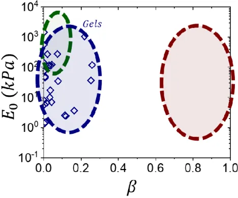
Figure 3.11: Populations of the elastic landscape ...28
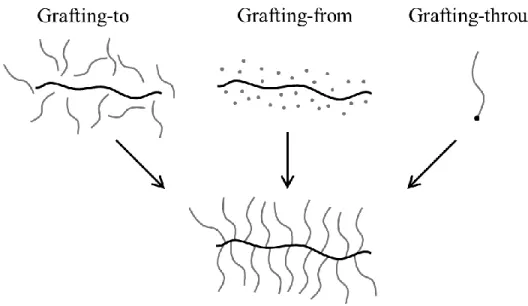
Figure 4.1: Different pathways to brushes ...30
Figure 4.2: Grafting-through brushes using controlled polymerizations ...32
Figure 5.1: Linear-brush-linear (LBL) self-assembled platform ...37
Figure 5.2: 1H-NMR of raw MCR-M11 and MCR-M17 PDMS macromonomers ...38
Figure 5.3: 1H-NMR of LBL plastomers at different stages of synthesis ...41
Figure 5.4: AFM of brushes ...42
Figure 5.5: AFM of self-assembled LBL domains ...43
Figure 5.6: USAXS of LBL plastomers with increasing 𝜙𝐿 decodes LBL firmness ...44
Figure 5.7: Representative stress-strain responses of MCR-M11 LBL plastomers...45
Figure 5.8: LBL plastomers bridge the firmness gap ...46
Figure 6.1: Tuning brush 𝑛𝑠𝑐 with mixtures of side chain lengths ...49
Figure 6.2: 1H-NMR growth of a random MMA and MCR-M11 mixed brush ...51
Figure 6.3: 1H-NMR of random MCR-M11 and MCR-M17 mixed brushes ...52
Figure 6.4: 1H-NMR of purified random MCR-M11 and MCR-M17 mixed brushes with an external reference ...54
Figure 6.5: Two-point 𝑛𝑠𝑐 calibration using pure MCR-M11 and MCR-M17 brushes ...55
Figure 6.6: Tracking growth of a random MCR-M11 and MCR-M17 mixed brush ...56
Figure 6.8: AFM characterization of random MCR-M11 and MCR-M17 mixed brushes ...58
Figure 6.9: X-ray characterization of pure MCR-M11 and MCR-M17 LBL plastomers ...59
Figure 6.10: X-ray 𝑑1 characterization of MCR-M11 and MCR-M17 mixed brushes ...60
Figure 6.11: Representative stress-strain responses of mixed brush LBL plastomers ...61
Figure 6.12: Programming the LBL platform to traverse the elastic landscape ...62
Figure 6.13: Universally collapsing the LBL platform ...63
Figure 6.14: Mimicking tissue mechanics with LBL plastomers ...64
Figure 6.15: LBL plastomer biocompatibility ...65
Figure 7.1: Elastic and yielding response of LBL plastomers ...67
Figure 7.2: X-ray under deformation ...68
Figure 7.3: Strain-rate dependence ...69
Figure 7.4: Hysteresis at large deformations ...69
Figure 7.5: Computer simulations of elastic and yielding responses ...70
Figure 7.6: A unified theory for the hierarchical deformation of LBL plastomers ...71
Figure 8.1: Different side chain arrangements ...72
Figure 8.2: Stress-strain of star-like MCR-M17 LBL plastomers ...74
Figure 8.3: The star-like transition on the elastic landscape ...75
Figure 8.4: Stress-strain of LBL plastomers with brush impurities ...76
xiii
Figure 8.6: 1H-NMR growth of LB1B2B1L MMA-M17-M11-M17-MMA pentablocks ...78
Figure 8.7: 1H-NMR growth of LB1B2B1L MMA-M11-M17-M11-MMA pentablocks ...79
Figure 8.8: Stress-strain responses of LB1B2B1L pentablock plastomers...80
Figure 8.9: LB1B2B1L pentablock plastomers on the elastic landscape ...81
Figure 8.10: Mixing brushes with different architectural parameters ...82
Figure 8.11: Stress-strain responses of LBL plastomers with strand mixtures...83
Figure 8.12: LBL plastomer strand mixtures on the elastic landscape ...84
Figure 8.13: Different LBL plastomer side chain arrangement on the elastic landscape ...85
Figure 9.1: LBL plastomer thermal stability ...87
Figure 9.2: Stress-strain responses of LBL plastomers with distinct L-block chemistry ...88
Figure 9.3: Highlighting tissue’s strength ...90
Figure 9.4: An LBL plastomer iteration with graft copolymers ...91
LIST OF ABBREIVATIONS AND SYMBOLS
2f-BiB ATRP difunctional initiator - ethylene bis(2-bromoisobutyrate) AFM Atomic force microscopy
AIBN Azobisisobutyronitrile
ATRP Atom transfer radical polymerization CDCl3 Deuterated chloroform
CTA Chain transfer agent
Ð Dispersity
DMA Dynamic mechanical analysis DP Degree polymerization 𝑑1 Inter-brush distance 𝑑2 Physical domain size 𝑑3 Linear-brush periodicity 𝐸 Structural modulus 𝐸0 Young’s modulus 𝐸1 Linear modulus
𝐸𝑒 Entanglement Modulus
Ebib ATRP monofunctional initiator - Ethyl α-bromoisobutyrate 1H-NMR Proton nuclear magnetic resonance
LB Langmuir-Blodgett technique LBL Linear-brush-linear
xv
MCR-M17 Monomethacryloxypropyl-terminated PDMS, 𝑀𝑛=5000g/mol Me6TREN ATRP ligand - tris[2-(dimethylamino) ethyl] amine
MMA Methyl methacrylate
𝑀𝑛 Number average molecular weight 𝑀𝑤 Weight average molecular weight
𝑛𝑏𝑏 Degree polymerization of a brush backbone 𝑛𝑐 Degree polymerization of brush cores
𝑛𝑒 Degree polymerization of polymer entanglements 𝑛𝑔 Grafting density of side chains
𝑛𝐿 Degree polymerization of linear blocks
𝑛𝑟 Number of elastic repeat units in graft copolymer brushes 𝑛𝑠 Degree polymerization of brush strands
𝑛𝑠𝑐 Number average degree polymerization of a side chain 𝑛𝑠𝑐,𝑛 Number average degree polymerization of a side chain 𝑛𝑠𝑐,𝑤 Weighted average degree polymerization of a side chain 𝑛𝑥 Degree polymerization between covalent cross-links PCL Poly(caprolactone)
PDMS Poly(dimethylsiloxane) PMMA Poly(methyl methacrylate) 𝑄 Linear block aggregation number 𝑄𝑠 Solvent fraction
RAFT Reversible addition fragmentation chain-transfer ROMP Ring opening metathesis polymerization
ROP Ring opening polymerization 𝑅𝑚𝑎𝑥 Poly chain contour length 𝑇𝑔 Glass transition temperature THF Tetrahydrofuran
𝑇𝑚 Melting temperature
USAXS Ultra-small angle X-ray scattering 𝛽 Strain stiffening or firmness parameter 𝛿 Solubility parameter
𝜆 Elongation ratio 𝜆𝑓𝑖𝑡 Elongation ratio fitting
𝜆𝑚𝑎𝑥 Maximum elongation ratio or extensibility 𝜎𝑚𝑎𝑥 Maximum true stress or strength
𝜎𝑡𝑟𝑢𝑒 True stress
1 CHAPTER 1
THE PURSUIT OF NATURE: INSPIRATIONS FROM TISSUE 1.1 Introduction
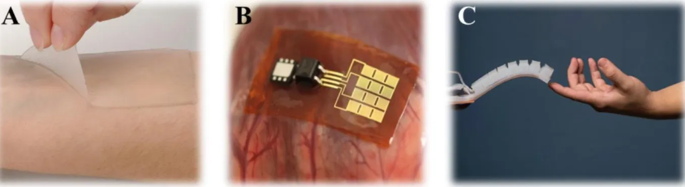
Biological tissues are an extraordinary class of materials with a unique set of mechanical properties. Although this is fairly self-evident, it is a valuable exercise to appreciate tissue’s mechanics with our own two hands by simply stretching and releasing the skin on the forearm. Outside of the pain likely felt, a few observations can be made. First, skin is initially relatively soft to touch compared to the hard materials we interact with in everyday life. Second, skin becomes increasingly difficult to stretch as it adaptively increases its stiffness with further deformation. Third, skin has incredible strength akin to hard rigid plastics. Finally, skin is resilient and quickly snaps back to its initial state upon release. These observations embody Nature’s key mechanical defense mechanism, which both prevents accidental tissue rupture while maintaining seamless interaction with the environment and serves as a benchmark for various industrial and biomedical applications. Specifically, mimicking tissue’s mechanical properties is of significant interest for use in topical adhesives, implantable and injectable devices and fillers, tissue scaffolds or replacements, and even in future soft robots (Figure 1.1). Therefore, mastering and encoding these mechanical features into synthetic systems is
Figure 1.1: Examples of applications requiring tissue-like materials. (A) Topical adhesives. (B) Implantable devices.1 (C) Soft robotics.2
1.2 Tissue Structure and Resulting Mechanics
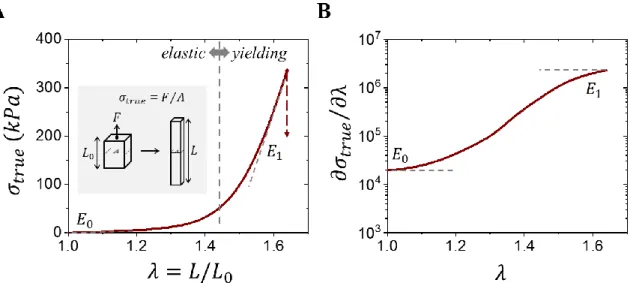
As demonstrated by the aforementioned skin stretching experiment (Section 1.1), soft tissues possess a distinct oxymoronic mechanical property combination: they are compliant at touch, yet resistant to deformation. With an initial slope or Young’s modulus (𝐸0) ranging from 103-107 Pa, biological tissues rapidly stiffen by a factor of 102-103 within a short interval. This can be observed in plots of true stress (𝜎𝑡𝑟𝑢𝑒), or the force response (F) over the changing cross-sectional area (A), produced by an applied strain (𝜀), or as interchangeably used in this
dissertation, the elongation ratio (𝜆 = 𝜀 + 1 = 𝐿/𝐿0) where the sample is deformed from its initial size 𝐿0 to length 𝐿 (Figure 1.2A).3-6 Tissue’s non-linear stress increase, or
strain-stiffening, holds true until an observed shift where tissue stress linearly scales with strain, known
respectively in tissue literature as the elastic and yielding regimes.5,6 As the name suggests, stretching and releasing within the elastic regime leads to a completely recoverable and
3
differential modulus (𝜕𝜎𝑡𝑟𝑢𝑒⁄𝜕𝜆) (Figure 1.2B), which highlights tissue’s characteristic
sigmoidal S-shape curve. Both the elastic regime’s Young’s Modulus (𝐸0) and yielding regime’s linear modulus (𝐸1) can be clearly identified to assist in comparing different tissue, however, a keen observer would realize these descriptors do not capture the shape of the stress-strain curve as addressed in Chapter 2 and demonstrated in Chapter 3.
Figure 1.2: Representative deformation response of tissues. (A) A representative stress-strain curve of a fetal membrane7 displaying an initial non-linear elastic regime and subsequent linear yielding regime, which is respectively characterized in the literature by the Young’s Modulus (𝐸0) and Linear modulus (𝐸1). (B) A corresponding differential modulus (𝜕𝜎𝑡𝑟𝑢𝑒⁄𝜕𝜆) plot shows tissue’s characteristic sigmoidal S-shape curve, which highlights 𝐸0 and 𝐸1.
triple helix held together by intramolecular hydrogen bonding (Figure 1.3A). The tropocollagen base unit then self-assembles into collagen microfibrils, which consist of five staggered and spiraled tropocollagen units. Lysine residues provide covalent crosslinking both within
microfibrils and with neighboring microfibrils to provide stability to the overarching structure. Assemblies of these collagen microfibrils then go on to align into variously sized macroscopic collagen fibers oriented in tissue.
Figure 1.3: Hierarchical structure of Collagen I. Collagen I is ordered at many different length scales: (A) Single protein strands made primarily of hydroxyproline-glycine-proline trimers coil into a tropocollagen helix serving as the base mechanical unit of collagen
macrostructure. (B) Individual tropocollagen self-assemble into collagen microfibrils via five staggered tropocollagen units in a cross-sectional area wrapped around each other like rope. Latent lysine units dispersed though tropocollagen strands chemically crosslink with neighboring tropocollagen helices. (C) Collagen microfibrils orient into individual fibers of different lengths also covalently crosslinked by lysine residues. These oriented bundles form the underlying structure of various tissues found throughout the body.
5
undeformed state at rest, the five wrapped tropocollagen in the microfibrils imperfectly self-assemble from both misalignments and kinks in individual tropocollagen helices (Stage I). Upon deformation, the misalignment is easily corrected with minimal forces imparting tissue’s softness (Stage II). After this adjustment has occurred, further extension causes the wrapped microfibril structure to uncoil and unravel as each individual rigid tropocollagen are stretched, which imparts the observed sharp strain-stiffening response (Stage III). Importantly, these three events represent purely elastic processes and with the release of strain will reversibly recover. When deformation forces become sufficiently large, the tropocollagen self-assembly breaks and strained tropocollagen units will begin sliding past each other, thus providing a linear yielding response (Stage IV). However, sliding eventually becomes impeded by the lysine covalent cross-links that break and lead to tissue rupture (Stage V).
response. Different mechanisms operate and activate at different stresses via either an elastic (Stage I-III) or yielding (Stage IV,V) process: (I) undeformed state where tropocollagen microfibrils are imperfectly coiled and contain misaligned kinks; (II) deformation straightens these kinks as tropocollagen helices align; (III) tropocollagen helices uncoil and begin stretching; (IV) critical stresses overcome tropocollagen self-assembly and enable sliding; (V) sliding
continues until lysine chemical links reach a maximum stress and results in either cross-link cleavage or rupturing tropocollagen strands inside the helix.
1.3 Summary and Outline
In summary, tissue’s remarkable hierarchical structure empowers a unique and unprecedented set of mechanical properties coveted by material scientists for use in future applications. Specifically, tissues possess a nearly identical chemical composition and water fraction, yet exhibit a broad range of mechanical properties (i.e. 𝐸0 = 103-107Pa), which
7
entire elastic landscape (Chapter 6), and qualitatively mimics tissue’s hierarchical deformation mechanisms (Chapter 7), with additional lessons learned regarding brush side chain
CHAPTER 2
THE ELASTIC LANDSCAPE: THEORETICAL INSIGHTS 2.1 Decoupling Softness and Firmness
A material’s strain-stiffening character, as introduced in Chapter 1, can be simplified as its ability to resist deformation. This description could also be also associated with a material’s initial softness or stiffness, however, as discussed in Chapter 1, the initial feeling of a material and its subsequent deformation response are two distinct concepts. Some literature13-15 and industrial16,17 sources recognize this distinction and aim to classify the resistance to deformation of various foods,14,16 mattresses,17 and our very own tissue15 (Figure 2.1) as firmness.
Figure 2.1: Colloquial examples using firmness. Firmness is used to describe (A) various food products including fruits and cheeses, (B) mattresses, and (C) tissues including skin.
To the native English speaker, this assigned name will likely cause confusion as
9
in magnitude, yet firmness is not softness. Although these sources13-17 correctly identify this distinction, they typically define firmness as the measured stress at a standard strain (i.e. 10%), 15-17 but this single point value provides some ambiguity (Figure 2.2). For instance, theoretical cases exist where two distinct materials with different initial slopes and different intensities of their strain-stiffening curvature may achieve identical firmness (Figure 2.2C). Furthermore, simply redefining the strain standard will deliver different firmness values. Therefore, the current description for firmness is neither robust nor complete, but two key features can be identified: (i) softness and firmness are distinct concepts, and (ii) firmness is related to the intensity of a material’s strain-stiffening curvature.
Two materials with both different Young’s modulus (𝐸0,𝑖 > 𝐸0,𝑖𝑖) and curvatures have identical firmness (𝜎𝑖 = 𝜎𝑖𝑖) according to the single point definition.
2.2 Redefining Firmness via an Elastic Model
In order to better quantify and compare different materials and material classes it is imperative to identify a theoretical model that precisely describes the entire stress-strain curvature and not simply as a single point value (Figure 2.2). Such a model will instruct intelligent and programmable design of desired stresses at various given strains in future
materials. Fortunately, theoreticians have developed an equation of state relating true stress 𝜎𝑡𝑟𝑢𝑒 with sample elongation ratio 𝜆 as shown in equation 2.1. 18,19
𝜎𝑡𝑟𝑢𝑒 = 𝐸 9(𝜆
2− 𝜆−1) (1 + 2 (1 − 𝛽(𝜆
2+ 2𝜆−1)
3 )
−2
) 2.1
11
brittle materials. This particular equation ignores the presence of trapped entanglements within the network, which may be accounted for with an additional fitting parameter,18 and is a concept discussed later (Section 3.3).
Figure 2.3: Physical origins of elastic parameters. (A) Structural modulus (𝐸) is classically related to the density of the material mesh size (1 𝑛⁄ 𝑥). (B) Strain-stiffening parameter (𝛽) is related to the initial conformation of individual strands 〈𝑅𝑖𝑛2〉 in relation to their contour length (𝑅𝑚𝑎𝑥) and is thus intimately related to material extensibility (𝜆𝑚𝑎𝑥).
A consequence of this model is the realization that a material’s Young’s modulus (𝐸0), depends not only on the cross-linking density (𝐸) but also on the initial strand conformation (𝛽) as highlighted in equation 2.2.
𝐸0 = 𝜕𝜎𝑡𝑟𝑢𝑒
𝜕𝜆 |𝜆→1 = 𝐸/3(1 + 2(1 − 𝛽)
−2) 2.2
Taking this one step further, combining both equations 2.1 and 2.2 into equation 2.3 yields an equation of state that provides two fitting parameters with observable features in stress-strain curves: the initial slope, or softness (𝐸0), and the following strain-stiffening curvature, or firmness (𝛽).
𝜎𝑡𝑟𝑢𝑒= 𝐸0
3(1 + 2(1 − 𝛽)−2)(𝜆
2− 𝜆−1) (1 + 2 (1 − 𝛽(𝜆2+ 2𝜆−1)
3 )
−2
) 2.3
(Figure 2.4B). In the first case, curves display an identical initial slope as designed, but distinct curvatures and extensibilities as higher 𝛽 materials show enhanced strain-stiffening and lower extensibilities. In the second case, curves display distinct initial slopes, but identical curvatures and extensibilities. These theoretical exercises delineate and validates the origins of the elastic curvature through the equation of state (equation 2.3) by eliminating the ambiguity surrounding the current usage of firmness as presented in Figure 2.2.
Figure 2.4: Theoretically constructed stress-strain curves. Varying fitting parameters of softness and firmness in equation 2.3 shows observable changes in theoretical stress-strain plots. (A) constant softness at different firmness or (B) different softness at constant firmness.
2.3 Conclusion and Outlook
This foundation for both the origin and mechanical characterization of polymer networks serves as a stepping stone to future intelligent material design. The elastic model both precisely characterizes a materials softness (𝐸0) and firmness (𝛽), and enables cataloging different material classes to streamline comparisons of large data sets in contrast to Edisonian approaches of
13
CHAPTER 3
INDEXING ELASTIC SYSTEMS: FROM TISSUE TO ELASTOMERS 3.1 Introduction
Various molecular and macroscopic constructs have endeavored to mimic the stress-strain behavior of tissue; however, most attempts rely on Edisonian approaches without
questioning the validity of the underlying platform. Therefore, before proposing an approach to achieve tissue softness and firmness, it is essential to first systematically characterize the mechanical limitations and boundaries of various material classes. Using the elastic model (Section 2.2), tissues (Section 3.2) are compared with different material classes including linear elastomers (Section 3.3), swollen elastomers or gels (Section 3.4), and the relatively young field of brush-like elastomers (Section 3.5).
3.2 Tissues
15
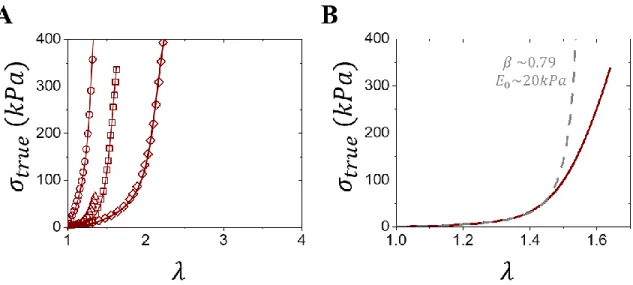
Figure 3.1: Characterizing tissue’s mechanical properties. (A) Stress-strain curves of various tissues including fetal membrane (squares),7 lens capsule (circles),24 muscle (triangle)25 and pig belly (diamonds).26 Note that connecting lines only serve to guide the reader and the chosen axis window does not fully capture every tissue’s stress-strain response. (B) Fitting of fetal membrane tissue using the elastic model to extract softness (𝐸0) and firmness (𝛽). Note that the model only characterizes elasticity and thus deviates during the yielding regime.
Both of the extracted fitting parameters from an ensemble of tissues found within the literature27 can be plotted onto an [𝐸0,𝛽] map, which highlights tissue’s mechanical boundaries of 𝐸0 = 103-107 Pa and 𝛽 > 0.7 (Figure 3.2). This realization may not at first seem that
Figure 3.2: Tissues on the elastic landscape. An [𝐸0,𝛽] map showing extracted elastic
parameters from various tissues (red circles).27 Most tissues show exceedingly high firmness (𝛽 > 0.7) and a wide softness range (𝐸0 = 103-107 Pa) revealing the tissue’s elastic zone.
3.3 Linear Elastomers
Elastomer networks constructed from chemically crosslinking linear strands has been ubiquitously used in various industrial applications (e.g. tires and rubber bands) ever since Goodyear first demonstrated vulcanization of natural rubber. Since then, the field of traditional linear elastomers has exploded to encompass numerous chemistries where rubbery polymers, i.e. neither crystalline (𝑇𝑚) nor glassy (𝑇𝑔) solids at normal operating temperatures, are coupled with various crosslinking schemes. These include historical sulfur crosslinking of unsaturated
17
which comprises various commercial brand names such as Sylgard, Ecoflex and Dragon Skin that persists into novel research to date.31,32 However, linear elastomers have an extremely narrow elastic range stemming from the lack of architectural control via their single classical network parameter of cross-linking density (𝑛𝑥) (Figure 3.3A). This limitation leads to two distinct issues: (i) crosslinking leads to permanent trapping of inherent strand entanglements and (ii) variations in 𝑛𝑥 lead to a coupled softness (network configuration) and firmness (strand conformation) (Section 2.2). The first issue is an unavoidable product of polymer physics as all polymer strands, regardless of chemistry, entangle at specific length scales (𝑛𝑒).33,34 Crosslinked elastomers naturally inherit this issue resulting in trapped entanglements that behave as
Figure 3.3: Physical limitations of linear elastomers. (A) Schematic of an elastomer network with programmable crosslinking density (𝑛𝑥) and inherent chain entanglements (𝑛𝑒) (B)
Representative plot of 𝑛𝑥 versus Young’s Modulus (𝐸0) in linear elastomers. Although
theoretical 𝑛𝑥 can be programmed via stoichiometry of various crosslinking strategies, a softness barrier (𝐸𝑒) is observed as inherent and unavoidable chain entanglements persist at large 𝑛𝑥 and behave as topological crosslinks. Note in linear elastomers, strand firmness is negligible (𝛽 → 0) and (𝐸0 ~ 𝐸).
The second issue arises as variations in 𝑛𝑥 both augment the density of mechanically active strands (Figure 2.3A) and individual strand conformations (Figure 2.3B), leading to a coupling of softness and firmness. This limitation follows classical intuition that hard networks are brittle and soft networks are extensible.34 Furthermore, attempts to increase material
19
Figure 3.4: Linear elastomers on the elastic landscape. An [𝐸0,𝛽] map showing linear elastomers (green squares).18,29 Linear elastomers face a softness barrier (𝐸0 > 105) and exceedingly low firmness (𝛽 < 0.1) unsuitable for matching tissue mechanics (red).
3.4 Synthetic Gels
spite of this improvement, gels face additional mechanistic and application issues. For instance, depending on the synthetic strategy, they inherit the entanglements from their linear network precursors (Figure 3.5) creating materials that are both soft but also very brittle as the entanglements become highly strained.34 Additionally, gel’s solvent fraction will inevitably evaporate or leak causing unwanted mechanical property drifting over time.
Figure 3.5: Synthetic gels: swelling linear networks. Schematic of swelling linear elastomers with solvent (blue circles), which (i) dilutes crosslinks toward lower softness and (ii) extends network strands toward higher firmness. Note that gels synthesized through linear elastomer swelling maintains the entanglements and imparts brittleness.
21
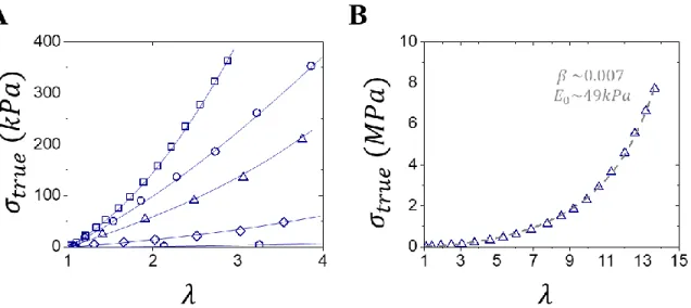
Figure 3.6: Characterizing gel’s mechanical properties. (A) Stress-strain curves of various gels including PEDOT/PSS (squares),37 PVA-PAAM (circles),38 PAAM-PAAc (triangles), 39 Polyrotaxane (diamonds) 40 and a clay nanocomposite (hexagons).41 Note that connecting lines only serve to guide the reader and the chosen axes window does not fully capture the entirety of every gel curve so as to match the window in Figure 3.1A. (B) Fitting of a PAAM-PAAc gel using the elastic model to extract softness (𝐸0) and firmness (𝛽). Note that the model fits the whole range in stark contrast with tissues.
The origin of this firmness divide stems from the weak strand extension of their linear chain networks, which mostly show 𝛽𝑑𝑟𝑦 ≅ 0.01, and the upper bound on their swelling ratio (𝛼 < 100). Taking these two limitations into consideration, a theoretical gel firmness barrier can be outlined according to equation 3.1 and is approximately 𝛽𝑔𝑒𝑙 < 0.2.27
𝛽𝑔𝑒𝑙 = 𝛽𝑑𝑟𝑦〈𝑅𝑖𝑛2 〉
𝑔𝑒𝑙⁄〈𝑅𝑖𝑛2〉𝑑𝑟𝑦 = 𝛽𝑑𝑟𝑦𝛼2 3⁄ 3.1
The observed firmness barrier may cause confusion as it is anticipated that network strands could conceivably swell and extend indefinitely to their extension limit 𝛽 → 1, however, a gel’s
maximum 𝑄𝑠 is a product of the balance between osmotic pressure and its swellability.29
within a given chemistry (Figure 3.7), albeit with significant firmness limitations 𝛽 < 0.2.27 This analysis does not include recent progress with more complex gel architectures such as dual network interpenetrating gels,42 and utilizing sacrificial bonds.43 Although, these reported systems also face similar elastic limitations (𝛽 < 0.4) and typically demonstrate high modulus due to initially high crosslink density.
Figure 3.7: Synthetic gels on the elastic landscape. An [𝐸0,𝛽] map showing extracted elastic parameters from various synthetic gels (blue diamonds).27 Gels enable piercing linear
elastomer’s softness barrier with comparable softness to tissue (𝐸0 = 103 - 106 Pa), and enhanced firmness albeit far from replicating tissue (𝛽 < 0.2).
3.5 The Brush-like Architecture
23
25
Therefore, the consequences of the brush architecture are two-fold: (i) the removal of the linear network entanglement barrier provides access to tissue-relevant softness, and (ii) grafted side chains behave analogously to solvent found in gels (Section 3.4). This second realization has important implications as side chains play a dual oxymoronic role to both dilute crosslinks towards tissue-relevant softness and extend network strands via side chain steric repulsion towards enhanced strand rigidity or firmness without the use of solvent. Furthermore, the
independent nature of the brush-like architectural triplet (𝑛𝑥, 𝑛𝑠𝑐, 𝑛𝑔) can be exploited to achieve fine-tuning of both softness and firmness independently.45,46 This was demonstrated by a model system utilizing a copolymer mixture of methacrylate end functionalized polydimethylsiloxane (PDMS) macromonomer with well-defined 𝑛𝑠𝑐, a butyl acrylate monomer spacer and
difunctional PDMS crosslinker in specified ratios via free radical polymerization to achieve various 𝑛𝑔 and 𝑛𝑥.45,46 For instance, softness may be held constant while tuning firmness
analogous to theoretical curves in Figure 2.4A, via simultaneous increases of 𝑛𝑥 and 𝑛𝑔 (Figure 3.9A). This occurs as the strand mass between crosslinks is held constant while the strand
Figure 3.9: Stress-strain responses of brush-like elastomers. Programming brush-like elastomers to have either (A) The same softness (𝐸0) by fixing the strand mass via
simultaneously increasing 𝑛𝑥 and 𝑛𝑔, and (B) the same firmness (𝛽) and extensibility by fixing the strand rigidity via counterbalancing 𝑛𝑥 and 𝑛𝑔.
27
Figure 3.10: Brush-like elastomers on the elastic landscape. An [𝐸0,𝛽] map showing extracted elastic parameters from various brush-like elastomers (orange triangles).45.46 Brush elastomers enable programmable solvent-free mimicking of gels thus providing comparable softness to tissue (𝐸0 = 103 - 106 Pa), but still far from replicating tissue firmness (𝛽 < 0.3).
3.6 Conclusion and Outlook
firmness. Despite the highlighted limitations, brush-like networks emerges as the most promising avenue given the elegant nature of the architecture’s programmable design.
29 CHAPTER 4
SYNTHETIC STRATEGIES FOR THE BRUSH ARCHITECTURE 4.1 Introduction
As the mechanical implications of the brush architecture are clearly outlined in Section 3.5, it is essential to speak briefly on the state-of-the-art of brush synthesis. Extensive literature reviews47-49 have already explored the different pathways to synthesize brushes with distinct chemistries and for various applications, yet it is imperative to ground the discussion within the goal of this dissertation. To this end, the limited elastic control of the chemically crosslinked brush elastomers described in Section 3.5 also has significant synthetic limitations that excludes careful characterization of the brush architectural parameters. Therefore, this chapter aims to refocus the discussion on a bottom up approach by first crafting well defined brushes that may then form materials to coverthe entire elastic landscape (Chapter 5,6).
4.2 A Brush Synthetic Strategies
Figure 4.1: Different pathways to brushes. Grafting well defined side chains to brush
backbone strands (left), growing side chains from brush backbones (middle) and grafting through end functionalized group of side chains.
31
suppress growth of shorter side chains that initiated later. Lastly, grafting-through utilizes polymer side chains with an end functionalized group that may be sequentially polymerized into well-defined brushes. This method often faces slow reaction times due to both the dilution of the functional end group and steric hindrance at the growing backbone end. Additionally, the most limiting feature is the challenge of purifying residual unreacted macromonomers from the brush mixtures, a similar problem faced in the grafting-to approach.
Various controlled polymerization schemes have been implemented to graft-through well-tailored brushes, however, few have emerged as effective strategies with wide chemical applicability and high degree of control. Premier examples include ring opening metathesis polymerization (ROMP),52 reversible addition-fragmentation chain transfer (RAFT), 53 and atom transfer radical polymerization (ATRP).54 To a reader versed in polymer synthesis, such complex systems are often restricted to small scales of the academic chemistry benchtop due to their costly initiators and catalysts. However, their industrial applicability is improved through the grafting-through approach as large macromolecules synthesized by traditional industrial approaches, such as ring opening polymerization (ROP) 55 and coordination-insertion polymerization (e.g. Ziegler-Natta), 56 dilute the costly requirements of the controlled polymerizations.
33
in literature.52 (B) Reversible addition-fragmentation chain transfer (RAFT) polymerization of macromonomers with a methacrylate end group using AIBN as an initiator and a generic RAFT chain transfer agent (CTA). Both the AIBN and CTA initiated brushes are shown in their “off” state. CTA specifics can be found in literature.53 (C) Atom transfer radical polymerization of macromonomers with a methacrylate end group using ebib as an initiator and a generic copper catalyst. Copper catalyst and ligand specifics can be found in literature.54
ROMP52 (Figure 4.2) is a polymerization technique that originated from the great success of small molecule metathesis, or rearrangement of olefin fragments, using various late transition metal catalysts and has expanded with the commercialization of improved Grubbs catalysts (G3). The synthetic strategy is now often employed in brush synthesis typically
leveraging the high ring strain of norbornene end functionalized macromonomers. However, one key issue is the catalyst also functions as the initiator, which remains tethered to the growing chain end and thus requires stoichiometric quantities per desired number of polymer strands. Additionally, ROMP limits backbone chemistries to strained rings (i.e. norbornene, cyclobutene, etc.) and requires end termination (e.g. with vinyl acetate) and further functionalization to enable sequential polymerization of different chemistries (e.g. methyl methacrylate).
polymer strands with homogenous end functionalization. Furthermore, the number of actively growing strands (i.e. “on”) are defined by the amount of added initiator and not the CTA, which creates a balance between reaction time and the end functionalization impurity described above.
ATRP54 (Figure 4.2) is a similar living radical polymerization where the transfer of a capping bromine from the growing chain end to a catalyst dictates the on-off state. Traditionally, ATRP catalysts are copper (I) species with complexing multidentate nitrogen ligands that tune the catalyst activity. In contrast to RAFT, monomer polymerization is more limited to
(meth)acrylates, styrene and acrylonitrile, but polymerization of monomers such as (meth)acrylamides and methacrylic acid are achievable with careful tuning of reaction
conditions. Unique to this polymerization, the catalyst can easily be purified and removed with fresh catalyst added to enable seamless continuation of the chain end polymerization on demand. Furthermore, the bromine end cap can easily undergo substitution to enable homogenous brush end functionalization.
4.3 Conclusion
35
CHAPTER 5
BRIDGING THE FIRMNESS GAP: LINEAR-BRUSH-LINEAR TRIBLOCKS 5.1 Introduction
Although the brush-like architecture offers an elegant foundation to independently
program softness and firmness into elastomers, it is necessary to bolster the architecture with
additional synthetic tools beyond what traditional elastomer networks can provide (Section 3.5).
Fortunately, a host of literature on self-assembled triblock copolymer physical networks provides
welcomed insight as the triblock structure has shown enhanced mechanical properties over their
covalently crosslinked counterparts.57-60 Thus, the brush-like architecture can be embedded into a
linear-brush-linear (LBL) ABA scaffold, which not only contain dissimilar chemical blocks but
also physically distinct architectures (Figure 5.1). The result is a highly tunable self-assembled
LBL thermoplastic elastomer (or plastomer) platform that has enhanced firmness empowered by
strong microphase separation. This platform maintains the brush-like architectural triplet of
brush length (𝑛𝑏𝑏), side chain length (𝑛𝑠𝑐) and grafting density (𝑛𝑔), while adding linear block length (𝑛𝐿) and corresponding volume fraction (𝜙𝐿). Self-assembly also enables observable physical features on length scales nontrivially related to the linear-brush periodicity (𝑑3), physical domain size (𝑑2), and inter-brush distance (𝑑1). The following sections will discuss a synthetic summary for LBL’s covered in this entire dissertation (Section 5.2), the structural and
37
Figure 5.1: Linear-brush-linear (LBL) self-assembled platform. (A) Representative synthetic scheme showing the sequential polymerization of the LBL platform (B) Programmable features of the LBL platform include brush length (𝑛𝑏𝑏), side chain length (𝑛𝑠𝑐), linear block length (𝑛𝐿) and volume fraction (𝜙𝐿), which self assembles into physical networks with nontrivially related physical parameters of linear-brush periodicity (𝑑3), physical domain size (𝑑2) and inter-brush distance (𝑑1).
5.2 LBL Plastomer Synthesis and Molecular Characterization
The procedures and expertise outlined herein serve as a general guiding principal for the synthesis of LBL plastomers. A full description and characterization of LBL plastomers with specific architectural parameters can be found in the literature.61
Typical LBL plastomers covered in this dissertation are synthesized from two components comprising each block: monomethacryloxypropyl-terminated
(MMA, 99%, ACROS) monomers as the linear L-block. This chemical combination is chosen as it shows a particularly strong phase separation.62 PDMS macromonomers are commercially available in two lengths as either MCR-M11 (Gelest, average molar mass 𝑀𝑛 = 1000 g/mol and dispersity, Ð =1.15) or MCR-M17 (Gelest, 𝑀𝑛 = 5000 g/mol and, Ð =1.15), with their corresponding 1H-NMR spectra in Figure 5.2. The side chain length (𝑛𝑠𝑐) of each is determined by the number of PDMS repeat units from 1H-NMR plus approximately 3 additional repeat units to account for the extra non-PDMS length (i.e. 11.4 + 3) to respectively yield 𝑛𝑠𝑐 = 14.4 and 71.2 for MCR-M11 and MCR-M17. Both the PDMS macromonomers and MMA should first be passed through a basic alumina column to remove radical inhibitor added by the suppliers.
Figure 5.2: 1H-NMR of raw MCR-M11 and MCR-M17 PDMS macromonomers. (400 MHz,
CDCl3): 6.12, 5.56 (CH2=C(CH3)C=O, s, 1H), 4.12 (CO-OCH2-, t, 2H), 3, 0.55 (-CH2
39
MCR-M17 (red)). 𝑛𝑠𝑐= [area(a)/6] + 3, providing 14.4 (MCR-M11) and 71.2 (MCR-M17) by approximating 3 additional repeat units comprise the side chain outside of PDMS.
An LBL plastomer is synthesized by sequential growth of the brush and then linear blocks via atom transfer radical polymerization (ATRP)54 using a difunctional initiator and a highly active copper complex to promote polymerization of the sterically hindered side chains. As an example, MCR-M11 (50.0 g, 50.0 mmol), ATRP difunctional initiator ethylene bis(2-bromoisobutyrate) (2f-BiB, 97%, Sigma Aldrich, 15mg, 41.6 µmol), ATRP ligand tris[2-(dimethylamino) ethyl] amine (Me6TREN, Sigma Aldrich, 19.2 mg, 22.2 µL, 83.3μmol) and toluene are bubbled with dry nitrogen for approximately 1 hour inside a Schlenk flask. Copper(I) bromide (Cu(I)Br, 99.999%, Sigma Aldrich, 8.3 mg, 83.3 µmol) is quickly added to the reaction mixture through the top of the flask. Subsequently, the flask is resealed, additionally purged with nitrogen for approximately 15 minutes, and then immersed in a 45 °C oil bath. The
polymerization is allowed to proceed with periodic samples taken from the nitrogen purged Schlenk arm and monitored by 1H-NMR. The polymerization is stopped by opening the flask and exposing the reaction mixture to air upon reaching the desired brush length (𝑛𝑏𝑏) (approximately 70-80% conversion), as determined by the disappearance of methacrylate end group (d) in
relation to the PDMS reference (a+a') (Figure 5.3). With the provided chemical quantities above, the brush length reaches approximately 𝑛𝑏𝑏 = 900 after 12 hours at 75% monomer conversion. Using this sequential growth process, it is imperative to remove residual unreacted
in a relatively similar fashion, as tracked by the emergence of PMMA (e') in reference to PDMS (a') within the brush (Figure 5.3). During this step, MMA can be added in excess (~1 brush mass equivalent) and the polymerization stopped with the desired 𝑛𝐿 or 𝜙𝐿 tracked by 1H-NMR. The resulting LBL is swelled and washed with excess acetone to remove MMA homopolymer as tracked by the disappearance of PMMA, then swelled and washed with excess hexane to remove unreacted PDMS bottlebrush as tracked by the increase in PMMA of the system, and dried overnight. Representative 1H-NMR spectra of each sequential polymerization and washing steps (unreacted macromonomer, brush growth, purified brush, unpurified LBL, LBL purified with acetone, LBL then
41
Figure 5.3: 1H-NMR of LBL plastomers at different stages of synthesis. For PDMS 𝑛
𝑠𝑐 = 70 (chapter 5) brushes (400 MHz, CDCl3): 6.12, 5.57 (CH2=C(CH3)C=O, PDMS macromonomer, s, 1H), 4.12 (CO-OCH2-, PDMS macromonomer, t, 2H), 0.55 (-CH2-(Si(CH3)2-O)n-CH2-CH2-, PDMS macromonomer and brush mixture, m, 4H) 0.09 (-(Si(CH3)2-O)n-, PDMS macromonomer and brush mixture, s, 438H). For PMMA-PDMS-PMMA (LBL) plastomer (400 MHz, CDCl3): 3.62 (COO-CH3, s, 3H), 0.55 (-CH2-(Si(CH3)2-O)n-CH2-CH2-, m, 2H) 0.09 (-Si(CH3)2-, s, 438H). 𝐶𝑜𝑛𝑣𝑃𝐷𝑀𝑆 = ([𝐴𝑟𝑒𝑎(𝑎 + 𝑎′)/438] − [𝐴𝑟𝑒𝑎(𝑑)/1]) [𝐴𝑟𝑒𝑎(𝑎)/438]⁄ . Peaks c' and 1 set of 2H b' for MCR-M17 brushes do not show on 1H-NMR in CDCl
3 in contrast to MCR-M11 brushes (see 5.2), 𝑛𝐿 = [𝐴𝑟𝑒𝑎(𝑒′)/3] [𝐴𝑟𝑒𝑎(𝑎)/438]⁄ ∗ 𝑛𝑏𝑏 where 𝑛𝑏𝑏 = 𝐶𝑜𝑛𝑣𝑃𝐷𝑀𝑆∗
[𝑀] [𝐼]. Subsequent washing with PDMS anti-solvent acetone and PMMA anti-solvent hexane removes acetone soluble PMMA homopolymer and hexane soluble PDMS brush, respectively.
5.3 LBL Physical Characterization
imaging of B-block brushes via atomic force microscopy (AFM) is made possible by exploiting the unique spreadability of brushes on substrates.63 Monolayers prepared by Langmuir-Blodgett (LB) techniques enable visual characterization of their worm-like brush backbones such as the series shown in Figure 5.4, which verifies increasing 𝑛𝑏𝑏 consistent with 1H-NMR.
Figure 5.4: AFM of brushes. Monolayers of MCR-M17 brushes (Section 6.2) with different brush lengths (𝑛𝑏𝑏) prepared by Langmuir-Blodgett (LB) technique. (A) 𝑛𝑏𝑏 = 100 (B) 𝑛𝑏𝑏 = 300 (C) 𝑛𝑏𝑏 = 450.
Furthermore, LBL plastomers can be self-assembled into thin films that may be probed via AFM by tapping into the films to reveal hard glassy PMMA L-block domains, such as the series in Figure 5.5 showing increasing 𝜙𝐿. Note that these images only elucidate the
43
Figure 5.5: AFM of self-assembled LBL domains. LBL plastomer thin films via drop-casting with increasing L-block volume fraction (𝜙𝐿). Domains are enhanced by exposing thin films to solvent vapors. (A) 𝜙𝐿 = 0.032 (B) 𝜙𝐿 = 0.055 (C) 𝜙𝐿 = 0.105.
LBL physical features are also probed via ultra-small-angle X-ray scattering (USAXS) to reveal order at various length scales nontrivially related to the linear-brush periodicity (𝑑3), characteristic ripples of monodisperse spherical domains (𝑑2) and inter-brush distance (𝑑1) (Figure 5.6A). Depending on the programmed dimensions, these lengths range from 𝑑3 = 40-150 nm, 𝑑2 = 20-40 nm and 𝑑1 = 3.4 nm for LBL’s synthesized with MCR-M11.61,64 In order to satisfy packing constraints within domain size 𝑑2, remarkable degrees of L-block strand
Figure 5.6: USAXS of LBL plastomers with increasing 𝝓𝑳 decodes LBL firmness. (A) Characteristic length scales of physical parameters are observed in X-ray traces including: inter brush distance (𝑑1), characteristic interference (form-factor) pertinent to the spherically-shaped domains (𝑑2), and domain-brush periodicity (𝑑3). (B) Strong microphase separation and high degree of packing at the linear-brush interface locally strains both the brush backbone and side chains into a nearly fully extended conformation.64
45
stress-strain responses can be measured under tension using a dynamic mechanical analysis (DMA) instrument from TA instruments. Unless otherwise stated, stretching experiments in this dissertation are performed at a strain rate of 0.005s-1. A representative series of LBL plastomers with distinct 𝑛𝑏𝑏 and similar 𝜙𝐿 cast in toluene (Figure 5.7) show significantly enhanced firmness relative to those observed by brush elastomers (Section 3.5).
Figure 5.7: Representative stress-strain responses of MCR-M11 LBL plastomers. All samples contain similar L-block volume fraction (𝜙𝐿) and distinct brush length (𝑛𝑏𝑏). Tuning these two parameters demonstrates adequate control over the LBL platform mechanics.
5.4 Summary and Implications
Figure 5.8: LBL plastomers bridge the firmness gap. An [𝐸0,𝛽] map showing LBL plastomers using MCR-M11 (black) in relation to all other classes of elastic materials tissue (red), linear elastomers (green), gels (blue) and brush-like elastomers (orange). LBL series include 𝑛𝑏𝑏 = 300 (squares), 600 (circles), 900 (triangles), 1200 (upside down triangles) with increasing 𝜙𝐿. The LBL platform successfully bridges the firmness gap between tissue and gels and improves upon brush elastomer firmness, however tuning of parameters 𝑛𝑏𝑏 and 𝜙𝐿 only leads to an observable coalescence of all materials and does not afford complete tuning over the entire [𝐸0, 𝛽] map.
47
CHAPTER 6
A PLATFORM TO TRAVERSE THE ENTIRE ELASTIC LANDSCAPE 6.1 Introduction
49
Figure 6.1: Tuning brush 𝒏𝒔𝒄 with mixtures of side chain lengths. Copolymerization of different (macro)monomers (𝑛𝑠𝑐= 1, 14, 70) enables tunable 𝑛𝑠𝑐 for implementation into the LBL scaffold (𝑛𝑏𝑏, 𝑛𝑠𝑐, 𝑛𝐿, 𝜙𝐿).
6.2 Synthesis of LBL Plastomers with Mixed Side Chains
The expertise outlined herein serves as a general guiding principal for the synthesis and characterization of LBL plastomers with mixed side chain lengths. Descriptions and
characterizations of LBL plastomers specifically with long side chains (MCR-M17) and other architecturally parameters can be found in the literature.27
Without repeating general LBL plastomer synthetic approaches presented in Section 5.2,
which largely remains the same, a few key distinctions should be highlighted for growing
brushes with mixed side chain lengths. First, macromonomer mixtures (i.e. MCR-M11 and
MCR-M17) are prepared by molar equivalents not mass equivalents to target desired 𝑛𝑠𝑐. Second, using volatile spacers, in this case MMA, requires reduced temperatures (e.g. dry ice in
acetone) during initial nitrogen purging to prevent evaporation, as evaporation which would
affect the mixture stoichiometry and final 𝑛𝑠𝑐. Third, it is prudent to use a different solvent system to facilitate mixtures containing long macromolecules due to the dilution of the
of anisole and toluene ranging between 100% toluene with pure MCR-M11, and 80% anisole
and 20% toluene with pure M17 is used. Note pure anisole is ill advised for PDMS
MCR-M17 macromonomers due to poor solubility. Finally, longer macromonomers require distinct
solvent systems for extracting residual unreacted macromonomer. In this case, sequential
methanol and isopropanol washes is an effective choice for respectively removing MCR-M11
and MCR-M17 macromonomers selectively from the final brush mixture.
In order to properly characterize the resulting copolymer brush, it is essential not only to
identify the final brush composition and conversion, but also the comonomer gradient during
growth as different length side chains are expected to polymerize at different rates due to dilution
of the end group. Copolymerization of MCR-M11 macromonomer and MMA spacer is relatively
trivial as their copolymerization can be separately identified as demonstrated in a representative
1H-NMR of a 25/75 mol% MMA/MCR-M11 stoichiometric mixture (Figure 6.2). This is
accomplished by sampling the brush mixtures during growth and subsequently evaporating
residual MMA monomer to yield a mixture of unreacted MCR-M11 macromonomer and the
MCR-M11/MMA brush. Although an expected slight enrichment of MMA spacer is initially
51
Figure 6.2: 1H-NMR growth of a random MMA and MCR-M11 mixed brush. (400 MHz,
CDCl3): 6.12, 5.56 (CH2=C(CH3)C=O, PDMS macromonomer, s, 1H), 4.12 (CO-OCH2-, PDMS
macromonomer, t, 2H), 3.91 (CO-OCH2-, PDMS brush, m, 2H), 3.62 (COO-CH3, MMA brush,
s, 3H), 0.55 (-CH2-(Si(CH3)2-O)n-CH2-CH2-, PDMS macromonomer and brush mixture, m, 4H)
0.09 (-(Si(CH3)2-O)n-, s, 68.4H). DPbbPDMS =
[area(a'+a)/68.4-area(d)/1]/[area(a'+a)/68.4]∗[PDMS]/[I], DPbbMMA = [area(e')/3]/[area(a'+a)/68.4] ∗[PDMS]/[I], 𝑛𝑏𝑏 = DPbbPDMS + DPbbMMA, Convbb= 𝑛𝑏𝑏/{([PDMS]+[MMA])/[I]}. ([PDMS]+[MMA])/[I] = 375, [PDMS]/[I] = 281.2.
Copolymerization and analysis of MCR-M11 and MCR-M17 macromonomer mixtures
presents a more complex challenge as it is impossible to decompose their signals in 1H-NMR. A
reader well versed in 1H-NMR may suggest comparing the PDMS polymer peak, which should
be a combination of the two raw polymer peaks in Figure 5.2, to a fixed discernable reference
that both macromonomers share, such as the hydrogens nearest the methacrylate end group that
shifts upon polymerization (c to c'). However, this suggestion breaks down given 1H-NMR of
increased longer side chain fractions. In fact, even the c' reference in pure MCR-M11 brushes
does not integrate to expectations. This problem is similarly observed in 1H-NMR of large
macromolecules studied in biochemistry,65 but is largely unaddressed in most brush synthetic
discussions. One possible explanation for this observation is that longer side chains shield the
backbone from resonating in 1H-NMR, but it ultimately remains a puzzling and unanswered
casualty of the brush synthesis that should be investigated by more qualified NMR experts.
Nevertheless, the 𝑛𝑏𝑏 can still be accurately determined from unpurified brush mixtures (Figure
6.3) as described in Section 5.2.
Figure 6.3: 1H-NMR of random MCR-M11 and MCR-M17 mixed brushes. (400 MHz,
CDCl3): 6.12, 5.56 (CH2=C(CH3)C=O, unreacted macromonomer, s, 1H), 4.12 (CO-OCH2-, t,
2H), 0.55 (-CH2-(Si(CH3)2-O)n-CH2-CH2-, m, 4H) 0.09 (-(Si(CH3)2-O)n-, PDMS macromonomer
and brush mixture, s, 68.4H - 409.2H depending on the stoichiometric ratio of added side chains). 𝑛𝑏𝑏 = [area(a'+a)/{corresponding stoichiometric
53
However, attempts to carefully measure final 𝑛𝑠𝑐 should be made in order to precisely and fully characterize the resulting brushes. In order to identify the final side chain composition, brush mixtures were first purified of residual macromonomers and a benzaldehyde external reference was added to each brush for further 1H-NMR analysis (Figure 6.4). As previously shown, the methacrylate backbone peak (c') does not provide a universal pathway for measuring these brushes, however the peak associated with hydrogens surrounding either side of the siloxane polymer (b to b') has a unique shift without additional extraneous overlap that provides a viable pathway. Indeed, the hydrogens nearest to the backbone partially resonate in pure MCR-M17 brushes, while all four hydrogens do resonate in pure MCR-M11 brushes. Therefore, the a'/b' ratio, or the PDMS polymer peak (a') related to the macromonomer (b') peak, (Figure 6.4) of pure MCR-M11 and MCR-M17 brushes can be correlated to their corresponding 𝑛𝑠𝑐 (Figure 6.5) to serve as a reference for brush mixtures. Here the a'/b' vs 𝑛𝑠𝑐 relationship can be
properties, whereby mixing side chains into brushes can be efficiently utilized to enable sweeping control over firmness (Section 6.3).
Figure 6.4: 1H-NMR of purified random MCR-M11 and MCR-M17 mixed brushes with an
external reference. (400 MHz, CDCl3): 8.16 (Bz, d, 2H), 7.64 (Bz, t, 1H), 7.51 (Bz, t, 2H), 4.12 (CO-OCH2-, t, 2H), 0.55 (-CH2-(Si(CH3)2-O)n-CH2-CH2-, m, 2H-4H, depending on effective
side chain length) 0.09 (-(Si(CH3)2-O)n-, brush, s, 68.4H - 409.2H depending on inclusion of side
55
Figure 6.5: Two-point 𝒏𝒔𝒄 calibration using pure MCR-M11 and MCR-M17 brushes. The a'/b' ratio may be utilized as a reference to determine true inclusion of both MCR-M11 and MCR-M17 into brushes synthesized with macromonomer mixtures.
Figure 6.6: Tracking growth of a random MCR-M11 and MCR-M17 mixed brush. (A) 1 H-NMR of an unpurified random brush to quantify brush growth and conversion (400 MHz, CDCl3): 6.12, 5.56 (CH2=C(CH3)C=O, s, 1H), 4.12 (CO-OCH2-, t, 2H), 0.55 (-CH2
-(Si(CH3)2-O)n-CH2-CH2-, m, 4H) 0.09 (-(Si(CH3)2-O)n-, PDMS macromonomer and brush mixture, s,
324H characteristic of a 25/75 MCR-M11/MCR-M17 mixture). (B) 1H-NMR of a purified random brush with external reference to quantify the side chain gradient during growth (400 MHz, CDCl3): 8.16 (Bz, d, 2H), 7.64 (Bz, t, 1H), 7.51 (Bz, t, 2H), 4.12 (CO-OCH2-, t, 2H), 0.55
(-CH2-(Si(CH3)2-O)n-CH2-CH2-, m, 2H-4H, depending on effective side chain length) 0.09
57
is input in to the two-point calibration (Figure 6.5) to determine 𝑛𝑠𝑐 of macromonomer mixtures. (C) conversion of a random brush from A versus calculated 𝑛𝑠𝑐 or fraction of MCR-M17 (𝜑17) from B.
For MMA and MCR-M11 mixed brushes, it is observed in 1H-NMR that growth of MMA linear (L) blocks (e'') superimpose with the MMA (e') contained in the brush (Figure 6.7), but both of these can be deconvoluted through careful initial characterization of the mixed brush (Figure 6.2). Interestingly, both types of PMMA are visually discernable in 1H-NMR as PMMA contained in linear blocks are sharp while PMMA contained in the brush are broad.
Figure 6.7: 1H-NMR of an LBL series using a random MMA and MCR-M11 mixed brush.
(400 MHz, CDCl3): 3.91 (CO-OCH2-, PDMS brush, m, 2H), 3.62 (COO-CH3, MMA brush and
linear mixture, s, 3H), 0.55 (-CH2-(Si(CH3)2-O)n-CH2-CH2-, m, 2H) 0.09 (-Si(CH3)2-, s, 68.4H).
6.3 Physical Characterization
Physical characterization techniques are largely identical to those described in Section 5.3; However, tuning 𝑛𝑠𝑐 affords discernable differences under AFM and USAXS. For instance, monolayers of MCR-M11 and MCR-M17 mixed brushes prepared by the LB method show increased spacing between neighboring backbones under AFM (Figure 6.8A). This spacing can be quantified and related to the increasing weight average side chain length (𝑛𝑠𝑐,𝑤) (Figure 6.8B) calculated from 1H-NMR (Figure 6.5), which is consistent with the thermodynamically preferred adsorption of longer side chains to substrates.66 The near linear correlation suggests that the calibration in Figure 6.5 is reasonable approximation.
Figure 6.8: AFM characterization of MCR-M11 and MCR-M17 mixed brushes. (A) Images of brush block monolayers showing increased interbrush distance with increased 𝑛𝑠𝑐 = 71.2 fraction. (B) Brush width determined by AFM as compared to weighted average side chain length (𝑛𝑠𝑐,𝑤) determined by 1H-NMR (Figure 5.4, 5.5) showing a non-linear correlation due to long side chains first adhering to substrates. Brushes with 𝑛𝑠𝑐 = 14.4 (green), 23.6 (navy), 33.8 (violet), 47.1 (pink) and 71.2 (black).
59
6.9). Increases in 𝑑3 from an increased 𝑛𝑠𝑐, where 𝑛𝑏𝑏 and 𝜙𝐿 are held relatively constant, suggest network strand extension and enhanced firmness empowered by a stronger microphase separation of more sterically hindered longer side chains. LBL’s from mixed MCR-M11 and MCR-M17 brushes also exhibit a consistent increase on length scales nontrivially related to the inter-brush distance (𝑑1) (Figure 6.10A) and follows theoretical predictions with number average side chain length (𝑛𝑠𝑐,𝑛) as 𝑑1 ~ 𝑛𝑠𝑐3/8 (Figure 5.10B).27,67
Figure 6.10: X-ray 𝒅𝟏 characterization of MCR-M11 and MCR-M17 mixed brushes. (A) Tracking increased interbrush distance peak (𝑑1). (B) Peak heights can be converted into 𝑑1 values, which are consistent with increasing number average side chain length (𝑛𝑠𝑐,𝑛) as predicted by theoretical considerations. Brushes with 𝑛𝑠𝑐,𝑛 = 14.4 (green), 23.6 (navy), 33.8 (violet), 47.1 (pink) and 71.2 (black).
Most importantly, the stress-strain responses were measured for an ensemble of mixed brush LBL plastomers programmed with 𝑛𝑏𝑏 = 200 - 450, 𝜙𝐿 = 0.02 - 0.1 and 𝑛𝑠𝑐 = 7.5 - 71.2, and cast in THF. A collection of stress-strain curves with similar 𝐸0 (Figure 6.11A) and similar 𝛽 (Figure 6.11B) highlights the versatility of varying 𝑛𝑠𝑐 with 𝜙𝐿. Note that similar 𝛽 does not equate to identical 𝜆𝑚𝑎𝑥 as predicted by theory (Section 2.2). This is explained by LBL
61
Figure 6.11: Representative stress-strain responses of mixed brush LBL plastomers. Varying the architectural parameters of 𝑛𝑠𝑐 and 𝜙𝐿 enable collections of either (A) LBL plastomers with similar 𝐸0 = 25kPa and different 𝛽, or (B) two groups of LBL plastomers (dashed vs solid line) respectively with similar 𝛽 = 0.77 and 𝛽 = 0.46 but different 𝐸0.
6.4 Summary and Applications
The extracted elastic parameters of an ensemble of LBL plastomers are shown on an [𝐸0, 𝛽] map in Figure 6.12. Successful variations of 𝑛𝑠𝑐, 𝑛𝑏𝑏 and 𝜙𝐿 yields many notable features: (i) vertical or lateral cross sections can respectively yield collections of materials similar to those found in Figure 6.11A,B, (ii) each series universally coalesce onto discrete lines for a given average 𝑛𝑠𝑐 (dashed lines Figure 6.12) (iii) increasing 𝑛𝐿or 𝜙𝐿 simultaneously increases 𝐸0 and 𝛽 up the coalesced line, while increasing 𝑛𝑏𝑏 simultaneously decreases 𝐸0 and 𝛽 down the coalesced line, and (iv) increasing 𝑛𝑠𝑐 laterally shifts the observed coalesced line towards higher 𝛽. These empirical correlations enable general design rules towards traversing the [𝐸0,𝛽]
boundaries are currently ill-defined and there likely exists a microphase regime change upon reaching high 𝜙𝐿 > 0.3. Comparison of these LBL plastomers with those in Figure 5.8, show a slight mismatch caused by the difference in casting solvent, which does not diminish the underlying importance of 𝑛𝑠𝑐 variation. Note that the vertical scale in Figure 6.12 is shortened for ease of viewing.
Figure 6.12: Programming LBL platform to traverse the elastic landscape. Elastic
63
Theoretical analysis27 enables universality for the overarching platform by correlating the attained mechanical properties with the corresponding architectural parameters (Figure 6.13) and serves as a foundation for fine-tuning future materials.
Figure 6.13: Universally collapsing the LBL platform. Theoretical considerations provide a direct route for universally programming the LBL platform, where 𝜑 = 𝑛𝑔⁄(𝑛𝑔+ 𝑛𝑠𝑐)
leach into the body,68,69 and which do not adequately mimic the mechanics of surrounding tissue.27
Figure 6.14: Mimicking tissue mechanics. (A) Selected true stress-strain curves of MCR-M17 LBL plastomers (lines) overlaid onto spinal cord,70 fetal membrane,7 and porcine brain71 tissues (symbols) found in the literature with similar mechanical properties. (B) Selected true stress-strain curves of MCR-M17 LBL plastomers (lines) match different types of adipose tissue72 (symbols).
The LBL platform also exhibits excellent biocompatibility as demonstrated by the
adhesion and proliferation of human normal mammary epithelial and adipose-derived
mesenchymal stem cells (MSCs) cultured onto an LBL plastomer surface with MCR-M17
brushes (Figure 6.15). Monitoring the cultured cells by fluorescence microscopy over the course
65
Figure 6.15: LBL plastomer biocompatibility. The proliferation of human normal mammary epithelial and adipose-derived mesenchymal stem cells cultured onto an LBL plastomer surface with MCR-M17 brushes and monitored by fluorescence microscopy after 1, 3, 5 and 7 days. Cells became confluent within 7 days.
CHAPTER 7
SEQUENTIAL DEFORMATION HIERARCHY OF LBL PLASTOMERS 7.1 Introduction