Oviedo University Press 24
Economics and Business Letters 7(1), 24-35, 2018
The intertemporal relation between expected returns and conditional
correlations between precious metals and the stock market
Ryuta Sakemoto*
YJFX Inc and Keio Economic Observatory, Keio University, Tokyo, Japan
Received: 30 December 2017 Revised: 15 April 2018 Accepted: 16 April 2018
Abstract
This study explores whether conditional correlations between precious metals and stock markets impact upon expected returns on precious metals. The empirical evidence presents that there is no significant trade–off between conditional correlations and expected returns. This study reveals that the impacts of conditional correlation are dependent upon the level of the expected returns. Interestingly, high absolute values of conditional correlations lead to increases in expected returns, suggesting that the unstable cross-asset market condition is associated with the expected returns. This result is due to a safe haven property for precious metals, and the impact is stronger on silver than on gold.
Keywords: gold; silver; precious metals; quantile regression; dynamic conditional correlation
JEL Classification Codes: B26, C21, G12, Q02
1. Introduction
Gold and silver have been used to store wealth for a long time. Recently, these precious metals have also been used to protect portfolio-wealth, since they are less correlated with other assets such as stocks, bonds and currencies. Baur and Lucey (2010) introduce the concept of a hedge and a safe haven, and investigate U.S., U.K. and German markets. They find that gold acts as a hedge and a safe haven in stock markets. Baur and McDermott (2010) examine many countries and confirm Baur and Lucey’s results. Furthermore, Joy (2011) adopts the dynamic conditional correlation approach and shows that gold works as a hedge tool for currency investors. Although these studies focus on gold, Agyei-Ampomah et al. (2014) address that silver also acts as a hedge for EU bond investors, and Sakemoto (2018) presents that silver has the same function for currency carry investors. Despite the diversification benefits of these precious metals to
* E-mail: [email protected]. The author would like to note that the views expressed in this paper are those of his own and do not necessarily represent those of YJFX Inc and Keio Economic Observatory.
investors, little is known about how these properties of precious metals affect their expected
returns.
The theoretical literature highlights that an asset which is highly correlated with the market portfolio bears a high expected return. Merton (1973) proposes the intertemporal capital asset pricing model (ICAPM) where a conditional expected return is dependent upon its conditional variance in order to satisfy a risk–return trade–off. The relation between conditional volatility and the expected return on stocks has been explored in the literature (e.g. French et al., 1987; Campbell, 1987; Glosten et al. 1993; Ghysels et al., 2005). In contrast, studies which focus on a relation between conditional covariance and the expected return are rare. One exception is Bail and Engle (2010) who present that conditional covariance is the source of positive equity premia. They find that high conditional covariance is associated with a high expected stock return.
This study extends the risk–return relation analysis to precious metals and investigates the relation between precious metals and the stock market, and how this affects the expected returns on precious metals. If there is a risk–return trade–off, high conditional covariance between pre-cious metals and stock markets will be linked to a high expected return on prepre-cious metals. Conditional covariance (correlation) between precious metals and the stock market is im-portant, since investors include precious metals in their portfolios in order to reduce portfolio risk levels. Our study motivates the intertemporal relation and investigates whether a high con-ditional correlation leads to a high expected return on precious metals due to increases in the risk level of the portfolio. The second contribution is that we focus on an asymmetric and non– linear relation between conditional correlations and expected returns. Quantile regressions are beneficial in capturing this asymmetric and non–linear relation, as shown by Baur (2013). This is desirable, since only a high–correlation period may affect expected returns. Moreover, high– and low– correlation periods may have different impacts on expected returns. For example, Rebored and Uddin (2016) reveal that the impact of financial stress differs throughout return quantiles of commodities. Thus, it is plausible to employ the quantile method in order to inves-tigate the asymmetric and non–linear relation.
The remainder of the paper is structured as follows. Section 2 describes estimation methods, and Section 3 explains datasets. Section 4 presents empirical results, and Section 5 concludes.
2. Methodology
2.1. Quantile regressions
This study investigates whether conditional correlations are associated with expected returns on precious metals. Merton (1973) proposes the ICAPM and implies that high conditional cor-relations lead to high expected returns on financial assets, since they are riskier for investors due to a lack of diversification benefits.
The relation between correlations and expected returns may depend upon a level of correla-tions, since only an extreme market condition affects expected returns. For instance, Aslanidis et al. (2016) employ a quantile regression approach and explore a risk–return relation in EU stock markets1. They report that as an expected return is extreme low, the impact of conditional
volatility is high.
This study follows Aslanidis et al. (2016) and adopts a quantile regression approach which estimates a degree and structure of dependence between two financial variables without assum-ing a certain structure of dependence (Baur, 2013; Mensi et al., 2014). This property is desirable in exploring asymmetric and non–linear effects of conditional variables. Quantile regressions proposed by Koenker and Bassett (1978) allow us to examine the impact of conditional varia-bles on expected returns in different market environments.
Let 𝜌𝑡be a conditional correlation between excess returns on stock and precious metal
mar-kets and the 𝜏–th conditional quantile excess return on the precious metal 𝑄𝑅𝑡+1(𝜏|𝜌𝑡) is
deter-mined as:
𝑄𝑅𝑡+1(𝜏|𝜌𝑡) = 𝛿(𝜏) + 𝛽(𝜏)𝜌𝑡 (1)
where 𝛿(𝜏)is the unconditional quantiles and each quantile has parameter 𝛽(𝜏). When the correlation and parameter 𝛽(𝜏)are positive,the high correlation leads to a high expected return.
2.2. Dynamic conditional correlation
Now, we move to an estimation method of conditional correlations. This study employs the Dynamic Conditional Correlation (DCC)–GARCH model proposed by Engle (2002). This ap-proach allows obtaining time–varying conditional correlations between stock and precious metal markets. Let 𝑟𝑚,𝑡+1 and 𝑟𝑖,𝑡+1 denote the excess returns on the stock market and that on the precious metal i at 𝑡 + 1, and the following mean return process is considered:
𝑦𝑡+1≡ (𝑟𝑟𝑚,𝑡+1
𝑖,𝑡+1) = 𝛼0+ 𝛼1𝑦𝑡+ 𝜀𝑡+1 (2)
where 𝜀𝑡+1 is the residual term and the conditional variance–covariance matrix of residuals
𝐻𝑡+1 is denoted as:
𝐻𝑡+1= 𝐷𝑡+1𝜌𝑡+1𝐷𝑡+1= {
ℎ𝑗,𝑡+1 𝑗 = 𝑘
ℎ𝑗,𝑡+11 2⁄ ℎ𝑘,𝑡+11 2⁄ 𝜌𝑖,𝑗 𝑗 ≠ 𝑘 (3)
where 𝐷𝑡+1 ≡ 𝑑𝑖𝑎𝑔(ℎ1,𝑡+1
1 2⁄
, ℎ2,𝑡+11 2⁄ ) is the diagonal matrix of conditional standard deviations
and 𝜌𝑡+1 is the conditional correlation matrix. Let ℎ𝑡+1 = [ℎ1,𝑡+1, ℎ2,𝑡+1 ] ′
and conditional vol-atility vector ℎ𝑡+1 is modelled as the GARCH (p,q) process2. Following Nakatani and Teräsvirta
(2009), volatility spillovers are taken into account, and the volatility vector is written as:
ℎ𝑡+1= 𝜔 + 𝐴𝜀𝑡2+ 𝐵ℎ𝑡
where 𝜔 = [𝜔𝜔1
2], 𝐴 = [
𝑎11 𝑎12
𝑎21 𝑎22], 𝐵 = [
𝑏11 𝑏12
𝑏21 𝑏22]
(4)
𝜔, 𝐴 and B are estimated parameters and off–diagonal elements 𝑎12, 𝑎21,𝑏12, and 𝑏21 capture
volatility spillovers. Conditional correlation matrix 𝜌𝑡+1is modelled as a function of lagged
standardised residuals 𝑢𝑡= 𝐷𝑡−1𝜀
𝑡, and lagged conditional correlation 𝜌𝑡:
𝜌𝑡+1 = 𝑆(1 − 𝛾1− 𝛾2) + 𝛾1𝑢𝑡𝑢𝑡′+ 𝛾
2𝜌𝑡 (5)
where 𝑆 is the unconditional correlation matrix of εt, and γ1 and γ2 are estimated parameters3.
3. Data
The data consist of daily gold and silver future prices against the U.S. dollar from Datastream. The sample period extends from 2 January 1978 to 31 January 2017. Daily excess returns are computed from S&P GSCI gold and silver indices. Recently, silver is also considered as an investment tool as reported by Lau et al. (2017), while silver is more affected by industrial demands4. For a stock market portfolio return, the value-weighted index for the Center for
2 This study assumes a GARCH (1,1) process.
3 We also employ the Asymmetric DCC-GARCH model proposed by Cappiello et al. (2006) and obtain the similar results.
Research in Security Prices (CRSP) is employed. For robustness, the Standard and Poor’s 500
(S&P 500) index is also used as a market portfolio. The one–month Treasury Bill rate is adopted as the risk–free rate.
4. Empirical results
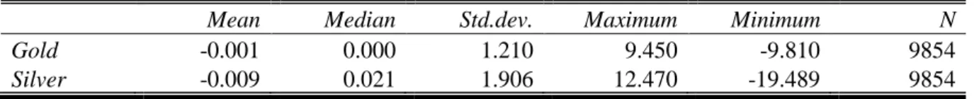
Table 1 reports the descriptive statistics of excess returns on gold and silver. Both mean returns are close to zero and the excess return on silver is more volatile than that of gold. Silver has a higher maximum value and a lower minimum value than gold.
Next, we demonstrate the estimation results of the DCC–GARCH model in Table 2. Both gold and silver results present that the diagonal elements of the GARCH term (𝐵) and those of the standard residuals (𝐴) in equation (4) are statistically significant at the 1% level, and the coefficients of the GARCH term (𝛾2) in equation (5) are persistent.
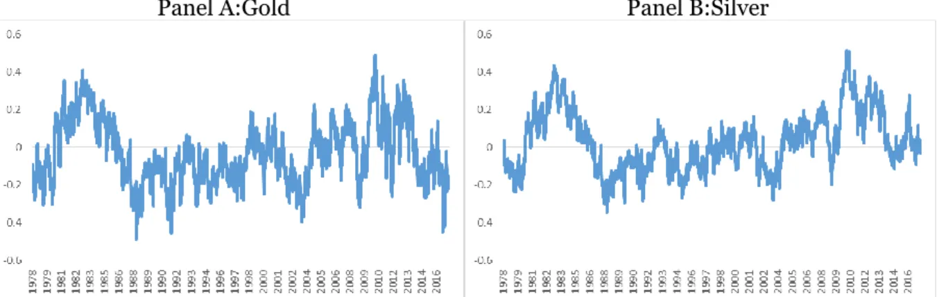
Figure 1 Panel A presents the estimated dynamic conditional correlation between the excess returns on gold and the stock market. The average correlation is negative, implying that gold works as a hedge against the stock market shock, and investors obtain the diversification benefit as suggested by Baur and McDermott (2010). However, the sign of the correlation sometimes flips; for example, it is positive around 1983 and 2010, which suggests that the hedging property of gold is time–varying.
Table 1. Descriptive statistics.
Mean Median Std.dev. Maximum Minimum N Gold -0.001 0.000 1.210 9.450 -9.810 9854
Silver -0.009 0.021 1.906 12.470 -19.489 9854
Note: Sample period is from 2 January 1978 to 31 January 2017.
Table 2. DCC–GARCH estimation results.
(1) (2)
mkt Gold mkt silver
ω 0.017 *** 0.002 0.019 *** 0.031 ** (0.004) (0.014) (0.005) (0.014)
A 0.091 *** 0.000 0.096 *** 0.000 (0.002) (0.002) (0.001) (0.001)
0.000 0.045 *** 0.000 0.056 *** (0.013) (0.001) (0.014) (0.007)
B 0.891 *** 0.001 0.887 *** 0.000 (0.005) (0.209) (0.019) (0.021)
0.002 0.954 *** 0.000 0.937 *** (0.305) (0.007) (0.007) (0.007)
γ1 0.017 *** 0.012 ***
(0.003) (0.002)
γ2 0.978 *** 0.985 ***
(0.004) (0.003)
log L -26,796 -31,784
Table 3. Regression results.
(1) (2)
Gold Silver
cons 0.000 -0.010
(0.013) (0.214)
dcc 0.020 0.020
(0.082) (0.143)
adj-R2 0.000 0.000
Note: This table shows the results for time series regression of the excess return on the lagged dynamic conditional correlation (dcc). Corresponding Newey and West (1987) standard errors are reported in parentheses.
Figure 1 Panel B demonstrates the dynamic conditional correlation between the excess re-turns on silver and the stock market. The correlation has a similar pattern to that of Panel A in Figure 1, although there are some differences. For instance, the correlation of gold reaches a more negative value than that of silver at the end of 1980s and around 2017.
Now, we explore the relations between the conditional correlation and the expected return on precious metals. The expected return is regressed on the conditional correlation as:
𝑟𝑖,𝑡+1 = 𝑎 + 𝑏𝜌𝑡+ 𝜀𝑡+1 (6)
where 𝑎 and 𝑏 are estimated parameters, and 𝜀𝑡+1 is an error term.
Table 3 presents the results of regressing excess returns on the lagged conditional correlations (dcc). Column (1) demonstrates the results of gold and column (2) does so of silver. Neither gold nor silver shows that the lagged conditional correlations are related to the expected returns, which means that the high conditional correlation does not generate the high expected return. This may imply that the conditional correlation impacts upon the expected return in only an extreme market situation. Recently, Aslanidis et al. (2016) report that impacts of conditional volatility depend upon the level of the expected return in the stock market context. We will investigate whether precious metals have the same property in the following analysis.
Our main interest in Table 4 is in employing quantile regressions and regressing the excess returns on precious metals on the lagged conditional correlations, and Table 4 presents slope parameter estimates at the 10th, 30th, 50th, 70th and 90th levels, which are given by equation (1). Standard deviations are reported in parentheses and estimated by the wild bootstrap ap-proach proposed by Feng et al. (2011). We begin with the results of gold and the empirical results reveal that all coefficients of dcc are statistically significant at the 1% level, except for the 50th quantile. Note that values of dcc have both negative and positive values. At the lower (upper) quantiles, the values of dcc tend to be negative (positive) and the coefficients of dcc increase monotonically.
Figure 1. Dynamic conditional correlations between excess returns on precious metals and the U.S. stock market.
We examine the impact in order to take into account both values of dcc and coefficients of
the quantile regressions. These results are reported in the row of impact in Table 4, which is calculated as the product of the i–th quantile of dcc and the coefficient. The empirical results reveal that extreme quantiles have higher impacts than middle do quantiles. For instance, at the 10th (90th) quantile, one unit of a negative (positive) change in dcc leads to an increase of the excess return by 0.23% (0.16%). In contrast, the impacts at the 30th and 70th quantiles are marginal. Interestingly, both high and low values of dcc lead to increases in the excess returns, which implies that the high excess returns do not come from high conditional correlations. The high excess returns are more related to the unstable cross-asset market environment. In other words, signs of the conditional correlations are not important but absolute values of those cause the high expected returns. Two factors may generate this empirical result. The positive relation between the excess return and the conditional correlation is explained by the ICAPM. Gold is an investing asset and has the same property with other assets. In contrast, the negative relation is associated with gold’s safe haven property. Baur and McDermott (2010) demonstrate that gold acts as a safe haven for a stock market in an extreme downside market condition. This is a unique characteristic for the precious metal, and is linked to the fact that the low correlation generates the high expected return on gold. Thus, the empirical result is partially explained by the ICAPM framework while the precious metal specific property is also important to determine the expected return. The empirical results of silver also present a similar pattern, while the im-pact is higher than that of gold at the extreme quantiles.
Next, we control for effects of other macroeconomic variables in Table 5. For potentially important variables in precious metal returns, we employ the following two variables: lagged U.S. stock market excess return (Batten et al, 2010) and lagged change in the U.S. long–term interest rate (Reboredo and Uddin, 2016). We observe that the dcc remains statistically signifi-cant and the magnitudes of coefficients are almost similar to those in Table 4. The lagged stock market excess return is positively associated with excess returns on gold and silver, which are statistically significant at the 1% level, except for gold in the upper quantile5. The impacts of
the interest rate are negative and strongly related to the excess returns at the upper quantiles. When the interest rate is high, investors prefer to invest in bonds so as to obtain income gains; thus, investors withdraw money from precious metal markets and invest in bond markets.
Table 4. Quantile regression results.
Quantiles Q(0.10) Q(0.30) Q(0.50) Q(0.70) Q(0.90) (1)Gold
cons -1.28 *** -0.39 *** 0.00 0.42 *** 1.29 *** (0.03) (0.03) (0.01) (0.01) (0.02)
dcc -0.96 *** -0.31 *** 0.00 0.40 *** 0.82 *** (0.14) (0.07) (0.04) (0.08) (0.11)
impact 0.23 0.04 0.00 0.02 0.16
(2)Silver
cons -2.12 *** -0.62 *** 0.02 0.70 *** 2.06 *** (0.04) (0.02) (0.01) (0.02) (0.04)
dcc -2.14 *** -0.60 *** 0.10 0.78 *** 1.80 *** (0.25) (0.13) (0.11) (0.12) (0.27)
impact 0.34 0.04 0.00 0.07 0.45
Note: This table shows estimates of quantile regressions in equation (1). Bootstrap standard errors are computed by Feng et al. (2011) and are reported in parentheses. impact indicates the magnitude (%) of one unit of change in the dynamic conditional correlation at the corresponding quantile. *, **, and *** indicates significance at the 10%, 5% and 1% level respectively.
Table 5. Quantile regression results with control variables.
Quantiles Q(0.10) Q(0.30) Q(0.50) Q(0.70) Q(0.90) (1)Gold
cons -1.29 *** -0.39 *** 0.00 0.42 *** 1.29 *** (0.03) (0.03) (0.01) (0.01) (0.02)
dcc -0.94 *** -0.34 *** 0.06 0.41 *** 0.82 *** (0.14) (0.07) (0.06) (0.07) (0.11)
mkt 0.07 *** 0.05 *** 0.03 *** 0.04 *** 0.01 (0.02) (0.01) (0.01) (0.01) (0.02)
int -0.40 -0.66 *** -0.68 *** -0.69 *** -0.93 *** (0.31) (0.14) (0.14) (0.19) (0.26)
impact 0.22 0.05 0.00 0.02 0.16
(2)Silver
cons -2.10 *** -0.63 *** 0.03 ** 0.69 *** 2.06 *** (0.04) (0.02) (0.01) (0.02) (0.04)
dcc -2.00 *** -0.64 *** 0.05 0.91 *** 1.72 *** (0.24) (0.13) (0.10) (0.14) (0.27)
mkt 0.27 *** 0.16 *** 0.10 *** 0.11 *** 0.17 *** (0.03) (0.02) (0.02) (0.02) (0.04)
int -1.09 *** -0.43 -0.35 *** -0.76 ** -1.12 ** (0.41) (0.31) (0.25) (0.32) (0.55)
impact 0.32 0.04 0.00 0.09 0.43
Note: This table shows estimates of quantile regressions in equation (1) with control variables, which includes the lagged CRSP stock market excess return (mkt) and the lagged change in the U.S. long–term interest rate (int). See notes in Table 4 for the other points. *, **, and *** indicates significance at the 10%, 5% and 1% level respectively.
5. Conclusion
This study investigates whether the dynamic conditional correlation between precious metal and stock markets is associated with expected returns on precious metals. Many investors have recently regarded precious metals as investment assets. Precious metals have an interesting property — they are used as a hedge against equity, bond and currency shocks. Thus, including precious metals in a portfolio reduces the portfolio’s risk level. This study examines whether the correlation between precious metal and stock markets affects expected returns on precious metals.
The empirical results reveal that there is no trade–off relation between the conditional corre-lation and the expected returns, while we observe that a high absolute value of the conditional correlation leads to an increase in the expected return. Our results suggest that the expected returns on precious metals are affected by the two factors. The first factor is the ICAPM. The second factor is a safe haven property of precious metals. As the stock market crashes, the high demand of precious metals results in the high expected returns on precious metals. The second factor is a unique property of precious metals and is new to the extant literature. Our empirical findings might be helpful to fund managers who estimate expected returns on precious metals in their portfolios.
Acknowledgements
References
Agyei-Ampomah, S., Gounopoulos, D., and Mazouz, K. (2014) Does gold offer a better protection against losses in sovereign debt bonds than other metals?, Journal of Banking and Finance, 40, 507-521.
Aslanidis, N., Christiansen, C., and Savva, C. (2016) Risk–return trade–off for European stock markets, International Review of Financial Analysis, 46, 84-103.
Bali, T.G., and Engle, R. F. (2010) The intertemporal capital asset pricing model with dynamic conditional correlations, Journal of Monetary Economics, 57. 377-390.
Batten, J.A., Ciner, C., and Lucey, B.M. (2010) The macroeconomic determinants of volatility in precious metals markets, Resources Policy, 35, 65-71.
Baur, D. G. (2013) The structure and degree of dependence: A quantile regression approach,
Journal of Banking and Finance, 37, 786-798.
Baur, D. G., and Lucey, B.M. (2010) Is gold a hedge or a safe haven? An analysis of stocks, bonds and gold, The Financial Review, 45, 217-229.
Baur, D. G., and McDermott, T.K. (2010) Is gold a safe haven? International evidence, Journal of Banking and Finance, 34, 1886-1898.
Campbell, J. Y. (1987) Stock returns and the term structure, Journal of Financial Economics, 18, 373-399.
Cappiello, L., Engle, R. F., and Sheppard, K. (2006) Asymmetric dynamics in the correlations of global equity and bond returns, Journal of Financial Econometrics, 537-572
Cenedese, G., Sarno, L., and Tsiakas, I. (2014) Foreign exchange risk and the predictability of carry trade returns, Journal of Banking and Finance, 42, 302-313.
Engle, R. F. (2002) Dynamic conditional correlation: a simple class of multivariate generalized autoregressive conditional heteroskedasticity models, Journal of Business and Economic Statistics, 20, 339-350.
Feng, X., He, X., and Hu, J. (2011) Wild bootstrap for quantile regression, Biometrica, 98, 995-999.
French, K., Schwert, G., and Stambaugh, R., (1987) Expected stock returns and volatility,
Journal of Financial Economics, 19, 3-29.
Ghysels, E., Santa-Clara, P., and Valkanov, R. (2005) There is risk–return trade–off after all,
Journal of Financial Economics, 76, 509-548.
Glosten, L.R., Jagannathan, R., and Runkle, D.E. (1993) On the relation between the expected value and the volatility of the nominal excess return on stocks, Journal of Finance, 48, 1779-1801.
Joy, M. (2011) Gold and the US dollar: Hedge or haven? Finance Research Letters, 8, 120-131.
Koenker, R., and Bassett, G. (1978) Regression quantiles, Econometrica, 46, 33-50.
Lau, M. C. K., Vigne, S. A., Wang, S., and Yarovaya, L. (2017) Return spillovers between white precious metal ETFs: The role of oil, gold, and global equity, International Review of Financial Analysis, 52, 316-332.
Mensi, W., Hammoudeh, S., Reboredo, J. C., and Nguyen, D. K. (2014) Do global factors impact BRICS stock markets? A quantile regression approach, Emerging Market Review, 19, 1-17.
Merton, R. (1973) An intertemporal capital asset pricing model, Econometrica, 41, 867-887. Nakatani, T., and Teräsvirta, T. (2009) Testing for volatility interactions in the constant
conditional correlation GARCH model, Econometrics Journal, 12, 147-163.
Reboredo, J. C., and Uddin, G.S. (2016) Do financial stress and policy uncertainty have an
impact on the energy and metals markets? A quantile regression approach, International Review of Economics and Finance, 43, 284-298.
Sakemoto, R. (2018) Do precious metals and industrial metal act as hedge and safe havens for currency portfolios? Finance Research Letters, 24, 256-262.
Appendix A - Asymmetric DCC–GARCH estimation
This study also employs the following Asymmetric DCC–GARCH proposed by Cappiello et al. (2006):
𝜌𝑡+1= 𝑆(1 − 𝛾1− 𝛾2) − 𝛾3𝑆−+ 𝛾
1𝑢𝑡𝑢𝑡′+ 𝛾2𝜌𝑡+ 𝛾3𝑢𝑡−𝑢𝑡−′ (A1)
where 𝑢𝑡− are the zero-threshold standardised residuals which are equals to 𝑢
𝑡 when less than
zero else zero otherwise, and 𝑆− is the unconditional correlation matrix of 𝑢 𝑡
−.
Table A1. Asymmetric DCC–GARCH estimation results.
(1) (2)
mkt gold mkt silver
Ω 0.019 *** 0.003 *** 0.019 *** 0.023 * (0.005) (0.001) (0.005) (0.013)
A 0.090 *** - 0.090 *** - (0.005) - (0.015) -
- 0.045 *** - 0.049 *** - (0.002) - (0.015)
B 0.892 *** - 0.891 *** - (0.016) - (0.015) -
- 0.954 *** - 0.945 *** - (0.001) - (0.018)
γ1 0.017 *** 0.012 *** (0.006) (0.003)
γ2 0.977 *** 0.985 *** (0.011) (0.004)
γ3 0.001 0.000
(0.002) (0.001)
log L -26,794 -31,838
Appendix B – Other empirical results
Table A2 shows estimates of quantile regressions in equation (1) with control variables, which includes the lagged S&P 500 excess return (sp) and the lagged change in the U.S. long–term interest rate (int). Bootstrap standard errors are computed by Feng et al. (2011) and are reported in parentheses. “Impact” indicates the magnitude (%) of one unit of change in the dynamic conditional correlation at the corresponding quantile. *, **, and *** indicates significance at the 10%, 5% and 1% level respectively.
Table A2. Quantile regression results with control variables.
Quantiles Q(0.10) Q(0.30) Q(0.50) Q(0.70) Q(0.90) Panel A: With control variables
(1) Gold
cons -1.29 *** -0.38 *** 0.00 0.42 *** 1.29 *** (0.03) (0.01) (0.01) (0.01) (0.02)
dcc -0.94 *** -0.34 *** 0.06 0.42 *** 0.89 *** (0.13) (0.08) (0.06) (0.07) (0.12)
sp 0.08 *** 0.05 *** 0.03 *** 0.04 *** 0.01 (0.02) (0.01) (0.01) (0.01) (0.02)
int -0.35 -0.60 *** -0.69 *** -0.60 *** -0.98 *** (0.29) (0.15) (0.12) (0.15) (0.25)
impact -0.94 -0.34 0.06 0.42 0.89
(2) Silver
cons -2.11 *** -0.63 *** 0.03 ** 0.70 *** 2.06 *** (0.04) (0.02) (0.01) (0.02) (0.04)
dcc -1.98 *** -0.67 *** 0.06 0.90 *** 1.71 *** (0.25) (0.13) (0.11) (0.14) (0.27)
sp 0.28 *** 0.15 *** 0.10 *** 0.10 *** 0.16 *** (0.04) (0.02) (0.02) (0.02) (0.04)
int -1.11 *** -0.36 -0.32 *** -0.75 ** -0.98 * (0.37) (0.27) (0.28) (0.35) (0.55)
impact -1.98 -0.67 0.06 0.9 1.71
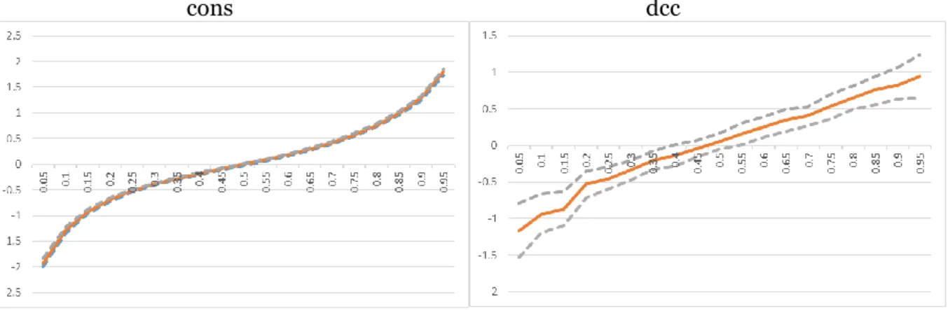
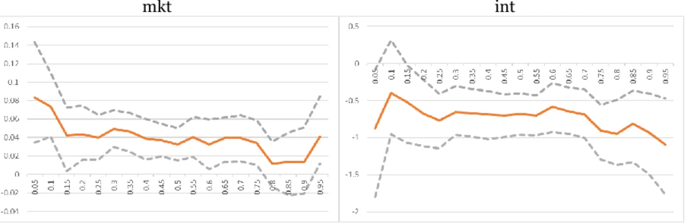
Figure A1. Quantile regression results with 95% confidence intervals for dynamic conditional correlations and control variables on the excess return of gold.
cons dcc
mkt int
Note. Dashed lines indicate 95% confidence intervals.
Figure A2. Quantile regression results with 95% confidence intervals for dynamic conditional correlations and control variables on the excess return of silver.
cons dcc
mkt int